Extinction theorem and propagation of electromagnetic waves between two semi-infinite anisotropic magnetoelectric materials

Abstract

Based on molecular optics we investigate the reflection and refraction of an electromagnetic wave between two semi-infinite anisotropic magnetoelectric materials. In terms of Hertz vectors and the principle of superposition, we generalize the extinction theorem and derive the propagation characteristics of wave. Using these results we can easily explain the physical origin of Brewster effect. Our results extend the extinction theorem to the propagation of wave between two arbitrary anisotropic materials and the methods used can be applied to other problems of wave propagation in materials, such as scattering of light.

I Introduction

In classical electromagnetism there are two well-known approaches to the propagation of electromagnetic waves. The first is to solve Maxwell’s equations with boundary conditions and the second is to use Ewald-Oseen extinction theorem of molecular optics theory Born . Compared to the former used traditionally, the latter can give much deeper physical insights into the interaction of electromagnetic wave with material Born ; Feynman1963 ; Wolf1972 ; Sein1972 ; Fearn1996 . Using the extinction theorem, the propagations of electromagnetic waves through a semi-infinite isotropic material Wolf1972 ; Reali1982 and an isotropic slab Lai2002 have been studied. Recently the Brewster mechanism is explained for light incident onto an isotropic material with negative index Fu2005 . The extinction theorem also plays a key role in light scattering theory Kong2001 .

In the previous works using the extinction theorem, most deal with the propagation of electromagnetic waves incident from free space into isotropic materials. However, the opposite situation from an material into free space and especially the situation between two materials is rarely studied. Then, whether the methods used in the previous work are applicable to the two situations? To answer this question, it is necessary to generalize the extinction theorem to investigate the propagation between two materials. On the other hand, a recent advent of artificial materials, named as negative-refraction materials, arouses many interest in the field of optics Veselago1968 ; Shelby2001 ; Pendry2000 ; Lindell2001 ; Smith2004 ; Luo2002 ; Hu2002 ; Lakhtakia2004 ; Lakhtakia2006 ; Lu2004 ; Luo2005 ; Luo2006a ; Luo2006b ; Shen2006 . Since the negative-refraction materials are actually anisotropic magnetoelectric, it is also necessary to extend the molecular optics from isotropic materials to anisotropic materials.

It is the purpose of this letter to use molecular optics to investigate systematically the propagation of electromagnetic wave between two semi-infinite anisotropic magnetoelectric materials. In terms of Hertz vectors and the principle of superposition we derive the properties of propagation and generalize the extinction theorem, so that the propagation between two arbitrary materials can be investigated in a unified framework of molecular optics. We also explain the mechanism of Brewster effect. The results extend the conclusions about the propagation in isotropic materials Fu2005 ; Lai2002 ; Reali1982 and throw light on those obtained by using Maxwell equations Shen2006 . The methods used do not require boundary conditions, but can reveal the interaction of light with materials, and avoid the difficulties in integrations and complex calculations usually encountered in using extinction theorem Wolf1972 . So the methods here can be applied to other problems of wave propagation in materials, such as scattering of light.

II Reflection, refraction, and extinction theorem

In this section, we first employ the formulation of Hertz vector and the principle of superposition to deduce the radiated fields generated by dipoles in the propagation of waves between two anisotropic dielectric-magnetic materials. Then we derive the real reflected and transmitted fields and the Fresnel’s coefficients. At the same time, we generalize the Ewald-Oseen extinction theorem. Throughout the paper SI units are used.

Let us consider a monochromatic electromagnetic field of ${\bf E}_{i}={\bf E}_{i0}\exp{(i{\bf k}_{i}\cdot{\bf r}-i\omega t)}$ and ${\bf H}_{i}={\bf H}_{i0}\exp{(i{\bf k}_{i}\cdot{\bf r}-i\omega t)}$ incident from an anisotropic material into another one filling the semi-infinite space $z>0$ with ${\bf k}_{i}=k_{ix}\hat{{\bf x}}-k_{iz}\hat{{\bf z}}$. The schematic diagram is in Fig. 1. Since the material responds linearly, all the fields have the same dependence of $\exp{(-i\omega t)}$ which will be omitted subsequently. For simplicity, the permittivity and permeability tensors of materials are assumed diagonal simultaneously in the principal coordinate system, $\bm{\varepsilon}_{j}=\hbox{diag}[\varepsilon_{jx},\varepsilon_{jy},\varepsilon_{jz}]$, $\bm{\mu}_{j}=\hbox{diag}[\mu_{jx},\mu_{jy},\mu_{jz}]$, $j=1,2$.

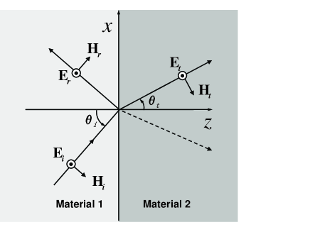
Figure 1: Schematic diagram for the reflection and refraction of TE waves at the interface between vacuum and an anisotropic material. The dashed line denotes the possible ray of negative refraction.

Following the molecular optics theory, a bulk material can be regarded as a collection of molecules (or atoms) embedded in the vacuum. Driven by the external field, the molecules are brought into oscillations and then secondary waves are generated by the induced dipoles. The radiated electric field by dipoles is decided by Born

$${\bf E}_{rad}=\nabla(\nabla\cdot{\bf{\Pi}}_{e})-\varepsilon_{0}\mu_{0}\frac{\partial^{2}{\bf{\Pi}}_{e}}{\partial t^{2}}-\mu_{0}\nabla\times\frac{\partial{\bf{\Pi}}_{m}}{\partial t}$$ (1)

and the generated magnetic field is

$${\bf H}_{rad}=\nabla(\nabla\cdot{\bf{\Pi}}_{m})-\varepsilon_{0}\mu_{0}\frac{\partial^{2}{\bf{\Pi}}_{m}}{\partial t^{2}}+\varepsilon_{0}\nabla\times\frac{\partial{\bf{\Pi}}_{e}}{\partial t}.$$ (2)

Here ${\bf\Pi}_{e}$ and ${\bf\Pi}_{m}$ are the Hertz vectors,

$${\bf\Pi}_{e}({\bf r})=\int\frac{{\bf P}({\bf r^{\prime}})}{\varepsilon_{0}}G({\bf r}-{\bf r}^{\prime})\hbox{d}{\bf r}^{\prime},$$ (3)

$${\bf\Pi}_{m}({\bf r})=\int{\bf M}({\bf r^{\prime}})G({\bf r}-{\bf r}^{\prime})\hbox{d}{\bf r}^{\prime}.$$ (4)

The dipole moment density of electric dipoles ${\bf P}$ and that of magnetic dipoles ${\bf M}$ are related to the associated field as ${\bf P}=\varepsilon_{0}\bm{\chi}_{e}\cdot{\bf E}$, ${\bf M}=\bm{\chi}_{m}\cdot{\bf H}$, where the electric susceptibility $\bm{\chi}_{e}=(\bm{\varepsilon}/{\varepsilon_{0}})-1$ and the magnetic susceptibility $\bm{\chi}_{m}=(\bm{\mu}/{\mu_{0}})-1$. The Green function is $G({\bf r}-{\bf r}^{\prime})=\exp{(ik_{0}|{\bf r}-{\bf r}^{\prime}|)}/(4\pi|{\bf r}-{\bf r}^{\prime}|)$, where $k_{0}$ is the wave number in vacuum. In the first medium the dipoles produce forward waves as well as backward waves. So, we assume the associated dipole moment densities have the following forms

$${\bf P}_{1} = {\bf P}_{1F}\exp{(i{\bf k}_{1F}\cdot{\bf r})}+{\bf P}_{1B}\exp{(-i{\bf k}_{1B}\cdot{\bf r})},$$

$${\bf M}_{1} = {\bf M}_{1F}\exp{(i{\bf k}_{1F}\cdot{\bf r})}+{\bf M}_{1B}\exp{(-i{\bf k}_{1B}\cdot{\bf r})},$$ (5)

while ${\bf P}_{2}={\bf P}_{2F}\exp{(i{\bf k}_{2F}\cdot{\bf r})}$ and ${\bf M}_{2}={\bf M}_{2F}\exp{(i{\bf k}_{2F}\cdot{\bf r})}$ in the second material, where $F$ and $B$ label the forward and backward propagating waves, respectively. We now determine the Hertz vectors. We firstly represent the Green function in the Fourier form Reali1982 . Then, inserting it into Eq. (3) and using the delta function definition and contour integration method, the Hertz vectors can be evaluated

$${\bf\Pi}_{1e}=\left\{\begin{array}[]{cc}\frac{{\bf P}_{1F}}{\varepsilon_{0}}\left[\frac{\exp{(i{\bf k}_{1F}\cdot{\bf r})}}{k_{1F}^{2}-q_{1F}^{2}}+\frac{\exp{(i{\bf q}_{1B}\cdot{\bf r})}}{2q_{1z}(q_{1z}+k_{1Fz})}\right]+\frac{{\bf P}_{1B}}{\varepsilon_{0}}\left[\frac{\exp{(-i{\bf k}_{1B}\cdot{\bf r})}}{k_{1B}^{2}-b_{1B}^{2}}+\frac{\exp{(-i{\bf b}_{1F}\cdot{\bf r})}}{2b_{1z}(b_{1z}-k_{1Bz})}\right],&z<0\\ -\frac{{\bf P}_{1F}}{\varepsilon_{0}}\frac{\exp{(i{\bf q}_{1F}\cdot{\bf r})}}{2q_{1z}(q_{1z}-k_{1Fz})}-\frac{{\bf P}_{1B}}{\varepsilon_{0}}\frac{\exp{(-i{\bf b}_{1B}\cdot{\bf r})}}{2b_{1z}(b_{1z}+k_{1Fz})},&z\geq 0\end{array}\right.$$ (8)

$${\bf\Pi}_{2e}=\left\{\begin{array}[]{cc}-\frac{{\bf P}_{2F}}{\varepsilon_{0}}\frac{\exp{(i{\bf q}_{2B}\cdot{\bf r})}}{2q_{2z}(q_{2z}+k_{2Fz})},&z<0\\ \frac{{\bf P}_{2F}}{\varepsilon_{0}}\left[\frac{\exp{(i{\bf k}_{2F}\cdot{\bf r})}}{k_{2F}^{2}-q_{2F}^{2}}+\frac{\exp{(i{\bf q}_{2F}\cdot{\bf r})}}{2q_{2z}(q_{2z}-k_{2Fz})}\right],&z\geq 0\end{array}\right.$$ (11)

where

$${\bf q}_{jF}=k_{jFx}\hat{{\bf x}}+q_{jz}\hat{{\bf z}},{\bf q}_{jB}=k_{jFx}\hat{{\bf x}}-q_{jz}\hat{{\bf z}},q_{jz}^{2}=k_{0}^{2}-k_{jFx}^{2},$$

$${\bf b}_{1F}=k_{1Bx}\hat{{\bf x}}+b_{1z}\hat{{\bf z}},{\bf b}_{1B}=k_{1Bx}\hat{{\bf x}}-b_{1z}\hat{{\bf z}},b_{1z}^{2}=k_{0}^{2}-k_{1Bx}^{2},j=1,2.$$ (12)

Following the superposition theory of field, the fields in the right region produced by the dipoles in the two media add up to the transmitted field. Then, we have

$${\bf E}_{t}={\bf E}^{1.right}_{rad}+{\bf E}^{2}_{rad},$$ (13)

where the contribution from the first medium to the right side, ${\bf E}^{1.right}_{rad}$, can be calculated by substituting Eq. (8) into Eq. (1)

$${\bf E}^{1.right}_{rad}=-\frac{{\bf Q}({\bf q}_{1F},{\bm{P}}_{1F})}{2q_{1z}(q_{1z}-k_{1Fz})}-\frac{{\bf Q}(-{\bf b}_{1B},{\bm{P}}_{1B})}{2b_{1z}(b_{1z}+k_{1Fz})},$$ (14)

the field radiated by the second medium itself, ${\bf E}^{2}_{rad}$, can be obtained after inserting Eq. (11) into Eq. (1)

$${\bf E}^{2}_{rad} = \frac{{\bf Q}({\bf k}_{2F},{\bm{P}}_{2F})}{k_{2F}^{2}-q_{2F}^{2}}+\frac{{\bf Q}({\bf q}_{2F},{\bm{P}}_{2F})}{2q_{2z}(q_{2z}-k_{2Fz})},$$ (15)

and ${\bf Q}$ is an auxiliary function

$${\bf Q}({\bf K},{\bm{P}})\equiv-\frac{1}{\varepsilon_{0}}\left[{\bf K}\times{\bf K}\times{\bm{P}}+({\bf K}^{2}-\varepsilon_{0}\mu_{0}\omega^{2}){\bm{P}}+\omega\mu_{0}\varepsilon_{0}{\bf K}\times{\bm{M}}\right]\exp{(i{\bf K}\cdot{\bf r})}$$ (16)

where ${\bf M}=\bm{\chi}_{m}\cdot\{{\bf k}\times[{\bf P}/(\varepsilon_{0}\bm{\chi}_{e})]/\bm{\mu}\}/\omega$. Substituting Eqs. (14) and (15) into (13), and considering the transmitted field with the form

$${\bf E}_{t}=\frac{{\bf P}_{2F}}{\varepsilon_{0}\bm{\chi}_{2e}}\exp{(i{\bf k}_{2F}\cdot{\bf r})},$$ (17)

we come to the following conclusions by a self-consistent analysis. (i). From terms with the phase factor $\exp{(i{\bf k}_{2F}\cdot{\bf r})}$ in Eq. (13) yield ${\bf k}_{2F}={\bf k}_{t}$ and the dispersion relation

$$\frac{k_{tx}^{2}}{\mu_{2z}\varepsilon_{2y}}+\frac{k_{tz}^{2}}{\mu_{2x}\varepsilon_{2y}}=\omega^{2},\frac{k_{tx}^{2}}{\varepsilon_{2z}\mu_{2y}}+\frac{k_{tz}^{2}}{\varepsilon_{2x}\mu_{2y}}=\omega^{2}$$ (18)

for TE and TM waves, respectively. (ii). We know that ${\bf q}_{1F}$, ${\bf q}_{2F}$ and ${\bf b}_{1B}$ are all vacuum wave vectors. Since only ${\bf k}_{2F}$ appears in the final transmitted field, they all should be extinguished. So we conclude that ${q}_{1z}={q}_{2z}=b_{1z}$ and $k_{1Fx}=k_{2Fx}=-k_{1Bx}$. Then, comes naturally the Snell’s law: $k_{1F}\sin\theta_{i}=k_{2F}\sin\theta_{t}$. At the same time,

$$\frac{{\bf Q}({\bf q}_{1F},{\bm{P}}_{2F})}{q_{1z}-k_{2Fz}}-\frac{{\bf Q}({\bf q}_{1F},{\bm{P}}_{1F})}{q_{1z}-k_{1Fz}}-\frac{{\bf Q}({\bf q}_{1F},{\bm{P}}_{1B})}{q_{1z}+k_{1Fz}}=0.$$ (19)

Equation (19) is the generalized expression of the extinction theorem about the forward vacuum waves. It describes how the radiation field produced by the dipoles of the first medium is extinguished by the counterpart in the second medium.

Now we study the fields in the first material. Similarly, all the fields radiated by the whole space are superposed to form the incident and reflected field.

$${\bf E}_{i}+{\bf E}_{r}={\bf E}^{1}_{rad}+{\bf E}^{2.left}_{rad},$$ (20)

where the field radiated by the first medium, ${\bf E}^{1}_{rad}$, can be calculated substituting Eq. (8) into Eq. (1)

$${\bf E}^{1}_{rad}=\frac{{\bf Q}({\bf k}_{1F},{\bm{P}}_{1F})}{k_{1F}^{2}-q_{1F}^{2}}+\frac{{\bf Q}({\bf q}_{1B},{\bm{P}}_{1F})}{2q_{1z}(q_{1z}+k_{1Fz})}+\frac{{\bf Q}(-{\bf k}_{1B},{\bm{P}}_{1B})}{k_{1B}^{2}-b_{1B}^{2}}+\frac{{\bf Q}({\bf q}_{1B},{\bm{P}}_{1B})}{2q_{1z}(q_{1z}-k_{1Bz})},$$ (21)

the contribution ${\bf E}^{2.left}_{rad}$ from the second medium to the left half-space can be obtained after inserting Eq. (11) into Eq. (1)

$${\bf E}^{2.left}_{rad} = -\frac{{\bf Q}({\bf q}_{2B},{\bm{P}}_{2F})}{2q_{2z}(q_{2z}+k_{2Fz})},$$ (22)

The incident and reflected fields may be written as

$${\bf E}_{i}=\frac{{\bf P}_{1F}}{\varepsilon_{0}\bm{\chi}_{1e}}\exp{(i{\bf k}_{1F}\cdot{\bf r})},{\bf E}_{r}=\frac{{\bf P}_{1B}}{\varepsilon_{0}\bm{\chi}_{1e}}\exp{(-i{\bf k}_{1B}\cdot{\bf r})},$$ (23)

respectively. Inserting Eqs. (21), (22) and (23) into (20) which must hold true for everywhere in the left half-space, we come to the following conclusions. (i). From terms with the phase factor $\exp{(i{\bf k}_{1F}\cdot{\bf r})}$ or $\exp{(i{\bf k}_{1B}\cdot{\bf r})}$ in Eq. (20) follow that ${\bf k}_{1F}={\bf k}_{i}$, ${\bf k}_{1B}={\bf k}_{r}$ and the dispersion relation is like Eq. (18) after replacing the subscripts 2 with 1 and $t$ with $i$, respectively. (ii). ${\bf q}_{1B}$ and ${\bf q}_{2B}$ are vacuum wave vectors and should be extinguished. So, we have ${\bf q}_{1B}={\bf q}_{2B}$ and

$$\frac{{\bf Q}({\bf q}_{1B},{\bm{P}}_{1F})}{q_{1z}+k_{1Fz}}+\frac{{\bf Q}({\bf q}_{1B},{\bm{P}}_{1B})}{q_{1z}-k_{1Fz}}-\frac{{\bf Q}({\bf q}_{1B},{\bm{P}}_{2F})}{q_{1z}+k_{2Fz}}=0,$$ (24)

which is a new expression of the extinction theorem we find. It shows how the the backward vacuum field produced by the dipoles of the second medium is extinguished by that in the first medium.

Solving the set of Eqs. (17), (19), (23), and (24), we obtain the reflection coefficient $R_{E}={E}_{r0}/{E}_{i0}$ and the transmission coefficient $T_{E}={E}_{t0}/{E}_{i0}$ for TE waves

$$R_{E}=\frac{\mu_{2x}k_{iz}-\mu_{1x}k_{tz}}{\mu_{2x}k_{iz}+\mu_{1x}k_{tz}},~{}~{}~{}T_{E}=\frac{2\mu_{2x}k_{iz}}{\mu_{2x}k_{iz}+\mu_{1x}k_{tz}}.$$ (25)

Analogously, we can discuss TM waves and obtain similar results after replacing $\bm{\mu}$ in with $\bm{\varepsilon}$, considering the expressions of ${\bf E}$ in Eq. (1) and ${\bf H}$ in Eq. (2).

Hence, we have obtained the generalized extinction theorem, i.e. Eqs. (19) and (24). So, the propagation between two arbitrary materials can be studied in a unified framework: Under the action of external field in the first material, the molecules in the tow materials are driven to oscillate and generate induced fields. The transmitted wave is the result of superposition of the incident vacuum field from the first medium and the fields radiated by the induced dipoles in the second medium. The reflected wave is the sum of the backward vacuum field from the second medium and the backward fields induced by the dipoles in the first medium. Note that Eqs. (19) and (24) should hold true for every point in the associated half-spaces, which indicates that the cancellation of vacuum waves occurs everywhere inside the materials.

III Origin of Brewster effect

In what follows we apply the above conclusions to discuss the origin of Brewster effect. If the power reflectivity $|R|^{2}=0$, there is no reflected wave and the incident angle is called Brewster angle Zhou2003 ; Grzegorczyk2005 ; Tamayama2006 ; Kong2000 . From Eqs. (24) follows the reflected field magnitude

$${\bf E}_{r0} = \frac{1}{q_{1z}+k_{iz}\mu_{0}/\mu_{1x}}\left\{\frac{{\bf q}_{1B}\times[{\bf q}_{1B}\times(\bm{\chi}_{1e}\cdot{\bf E}_{i0})]}{q_{1z}+k_{iz}}+\frac{{\bf q}_{1B}\times\{\bm{\chi}_{1m}\cdot[{\mu_{0}}{\bm{\mu}}_{1}^{-1}\cdot({\bf k}_{i}\times{\bf E}_{i0})]\}}{q_{1z}+k_{iz}}\right.$$ (26)

$$\left.+\frac{{\bf q}_{1B}\times[{\bf q}_{1B}\times(\bm{\chi}_{2e}\cdot{\bf E}_{t0})]}{q_{1z}+k_{tz}}+\frac{{\bf q}_{1B}\times\{\bm{\chi}_{2m}\cdot[{\mu_{0}}{\bm{\mu}}_{2}^{-1}\cdot({\bf k}_{t}\times{\bf E}_{t0})]\}}{q_{1z}+k_{tz}}\right\}.$$

On the right-hand side of Eq. (26), the first two denote the contributions (labelled as ${\bf E}^{i}_{r0}$) of dipoles in the first medium to the reflected field, while the last two are the contributions (labelled as ${\bf E}^{t}_{r0}$) from the second medium. In order for zero reflection, it requires that ${\bf E}^{i}_{r0}+{\bf E}^{t}_{r0}=0$, from which follows the condition for Brewster effect: If

$$\frac{\mu_{2z}\varepsilon_{2y}-\mu_{1z}\varepsilon_{1y}}{\mu_{1z}\mu_{2z}(\mu_{2x}\varepsilon_{1y}-\mu_{1x}\varepsilon_{2y})}>0,$$ (27)

the Brewster angle for TE waves is

$$\theta_{B}^{TE}=\cot^{-1}\sqrt{\frac{\mu_{1x}^{2}(\mu_{2z}\varepsilon_{2y}-\mu_{1z}\varepsilon_{1y})}{\mu_{1z}\mu_{2z}(\mu_{2x}\varepsilon_{1y}-\mu_{1x}\varepsilon_{2y})}}\,;$$ (28)

If $\mu_{2x}/\mu_{1x}=\varepsilon_{2y}/\varepsilon_{1y}\cap\varepsilon_{2y}/\varepsilon_{1y}\neq\mu_{1z}/\mu_{2z}$, then $\theta_{B}^{TE}=0$; When $\mu_{2x}/\mu_{1x}\neq\varepsilon_{2y}/\varepsilon_{1y}\cap\varepsilon_{2y}/\varepsilon_{1y}=\mu_{1z}/\mu_{2z}$, $\theta_{B}^{TE}=\pi/2$; If $\mu_{2x}/\mu_{1x}=\varepsilon_{2y}/\varepsilon_{1y}\cap\varepsilon_{2y}/\varepsilon_{1y}=\mu_{1z}/\mu_{2z}$, then Brewster effect will occur for any angle of incidence, which may lead to important applications in optics. All the typical and nontrivial sign combinations of $\bm{\varepsilon}$ and $\bm{\mu}$ are shown in Table. 1.

Table 1: Existence conditions of Brewster angles for TE waves at the interface of two anisotropic media. 

$\mu_{1x}$	$\mu_{1z}$	$\varepsilon_{1y}$	$\mu_{2x}$	$\mu_{2z}$	$\varepsilon_{2y}$	Existence conditions
$+$	$+$	$+$	$+$	$+$	$+$	$\frac{\mu_{2x}}{\mu_{1x}}>\frac{\varepsilon_{2y}}{\varepsilon_{1y}}\cap\frac{\varepsilon_{2y}}{\varepsilon_{1y}}>\frac{\mu_{1z}}{\mu_{2z}}$, $\frac{\mu_{2x}}{\mu_{1x}}<\frac{\varepsilon_{2y}}{\varepsilon_{1y}}\cap\frac{\varepsilon_{2y}}{\varepsilon_{1y}}<\frac{\mu_{1z}}{\mu_{2z}}$
$+$	$+$	$+$	$-$	$+$	$+$	$\frac{\varepsilon_{2y}}{\varepsilon_{1y}}<\frac{\mu_{1z}}{\mu_{2z}}$
$+$	$+$	$+$	$+$	$-$	$+$	$\frac{\mu_{2x}}{\mu_{1x}}>\frac{\varepsilon_{2y}}{\varepsilon_{1y}}$
$*$	$*$	$*$	$+$	$+$	$-$	$\times$
$+$	$+$	$-$	$*$	$*$	$*$	$\times$
$+$	$+$	$+$	$+$	$-$	$-$	$\frac{\varepsilon_{2y}}{\varepsilon_{1y}}>\frac{\mu_{1z}}{\mu_{2z}}$
$+$	$+$	$+$	$-$	$+$	$-$	$\frac{\mu_{2x}}{\mu_{1x}}<\frac{\varepsilon_{2y}}{\varepsilon_{1y}}$
$+$	$-$	$+$	$+$	$-$	$+$	$\frac{\mu_{2x}}{\mu_{1x}}<\frac{\varepsilon_{2y}}{\varepsilon_{1y}}\cap\frac{\varepsilon_{2y}}{\varepsilon_{1y}}>\frac{\mu_{1z}}{\mu_{2z}}$, $\frac{\mu_{2x}}{\mu_{1x}}>\frac{\varepsilon_{2y}}{\varepsilon_{1y}}\cap\frac{\varepsilon_{2y}}{\varepsilon_{1y}}<\frac{\mu_{1z}}{\mu_{2z}}$
$+$	$-$	$+$	$-$	$+$	$+$	$\forall$
$-$	$+$	$+$	$-$	$+$	$+$	$\frac{\mu_{2x}}{\mu_{1x}}<\frac{\varepsilon_{2y}}{\varepsilon_{1y}}\cap\frac{\varepsilon_{2y}}{\varepsilon_{1y}}>\frac{\mu_{1z}}{\mu_{2z}}$, $\frac{\mu_{2x}}{\mu_{1x}}>\frac{\varepsilon_{2y}}{\varepsilon_{1y}}\cap\frac{\varepsilon_{2y}}{\varepsilon_{1y}}<\frac{\mu_{1z}}{\mu_{2z}}$
$+$	$+$	$+$	$-$	$-$	$-$	$\frac{\mu_{2x}}{\mu_{1x}}>\frac{\varepsilon_{2y}}{\varepsilon_{1y}}\cap\frac{\varepsilon_{2y}}{\varepsilon_{1y}}>\frac{\mu_{1z}}{\mu_{2z}}$, $\frac{\mu_{2x}}{\mu_{1x}}<\frac{\varepsilon_{2y}}{\varepsilon_{1y}}\cap\frac{\varepsilon_{2y}}{\varepsilon_{1y}}<\frac{\mu_{1z}}{\mu_{2z}}$
$+$	$-$	$+$	$+$	$-$	$-$	$\forall$
$+$	$-$	$+$	$-$	$+$	$-$	$\frac{\mu_{2x}}{\mu_{1x}}>\frac{\varepsilon_{2y}}{\varepsilon_{1y}}\cap\frac{\varepsilon_{2y}}{\varepsilon_{1y}}>\frac{\mu_{1z}}{\mu_{2z}}$, $\frac{\mu_{2x}}{\mu_{1x}}<\frac{\varepsilon_{2y}}{\varepsilon_{1y}}\cap\frac{\varepsilon_{2y}}{\varepsilon_{1y}}<\frac{\mu_{1z}}{\mu_{2z}}$
$+$	$-$	$-$	$-$	$+$	$+$	$\frac{\mu_{2x}}{\mu_{1x}}<\frac{\varepsilon_{2y}}{\varepsilon_{1y}}\cap\frac{\varepsilon_{2y}}{\varepsilon_{1y}}>\frac{\mu_{1z}}{\mu_{2z}}$, $\frac{\mu_{2x}}{\mu_{1x}}>\frac{\varepsilon_{2y}}{\varepsilon_{1y}}\cap\frac{\varepsilon_{2y}}{\varepsilon_{1y}}<\frac{\mu_{1z}}{\mu_{2z}}$

Note: $*$ denotes either of $\pm$, $\forall$ indicates that Brewster angle exists for any parameter values.

Note that, if the first medium is vacuum, ${\bf E}^{i}_{r0}=0$, then zero-reflection can occur only when ${\bf E}^{t}_{r0}=0$. In other words, the Brewster effect is because the contributions from electric and magnetic dipoles of the medium to the reflected field in vacuum add up to zero, which is also pointed out in Ref. Fu2005 . In order to describe these conclusions, we give numerical examples in Fig. 2.

Figure 2: Reflectivity and reflected field magnitudes, normalized by the corresponding incident field magnitudes, for TE wave incident incident on the interface between two anisotropic materials. The three curves of reflectivity in (a) correspond the case in (b), (c), and (d), respectively. Since the first medium is vacuum in (b), the radiated electric fields (${\bf E}^{t}_{r0}$) generated by the second medium forms the reflected field, then Brewster angle $\theta_{B}^{TE}$ appears when ${\bf E}^{t}_{r0}=0$. In (c), $\theta_{c}$ is the critical angle of incidence. In (d), ${\bf E}^{i}_{r0}+{\bf E}^{t}_{r0}\equiv 0$, so omnidirectional total transmission occurs.

We also follow the method in Ref. Lu2004 to simulate in Fig. 3 a beam ${\bf E}_{i}={\bf E}_{i0}\int\hbox{d}k_{\perp}e^{i({\bf k}_{0}+{\bf k}_{\perp})\cdot{\bf r}}f({k}_{\perp})$ incident from an anisotropic material to another where $f({k}_{\perp})$ is the Gaussian modulation. We can see numerical simulations are in agreement with the theoretical conclusions. Experimentally Brewster effect has been realized with metamaterials Tamayama2006 . So, one can realize zero reflection through choosing appropriate material parameters, which may lead to make polarizers or light splitters.

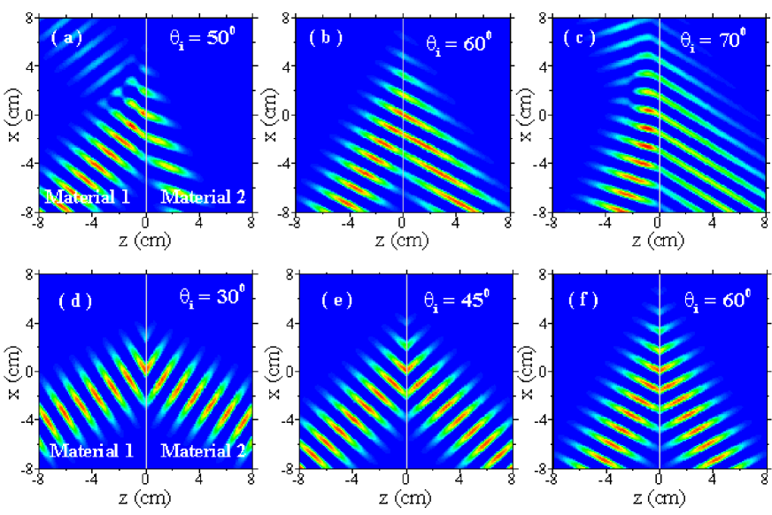
Figure 3: Reflection and refraction of a Gaussian beam incident on the interface between two anisotropic materials. For (a)-(c) and (d)-(f) the two materials correspond to those in (c) and (d) of Fig. 2, respectively. The phase and the energy flow are refracted regularly and anomalously, respectively in (a)-(c), but are both refracted anomalously in (d)-(f).

IV Conclusion

In summary, we carried out a systematical investigation on the propagation of wave between two anisotropic magnetoelectric materials. In terms of Hertz vectors and the principle of superposition we derive the properties of propagation and generalize the extinction theorem, so that the propagation between two arbitrary materials can be investigated in a unified framework. We apply the results to explain the physical origin of Brewster effect. The methods do not require boundary conditions, but can disclose the microscopic process of light propagation in materials, and avoid complex calculations usually encountered in using the extinction theorem. So the methods can be applied to other problems of wave propagation, such as scattering of light Kong2001 , propagation through stratified media Karam1996 or metamaterials Belov2006 , and so on.

- (1) M. Born and E. Wolf, Principles of Optics, 7th ed. (Cambridge, Cambridge, 1999).
- (2) R. P. Feynman, R. B. Leighton, and M. Sands, The Feynman Lectures on Physics (Addison-Wesley, 1963), Vol. 1, Secs. 31 and 30-7.
- (3) E. Lalor and E. Wolf, J. Opt. Soc. Am. 62, 1165 (1972).
- (4) J. L. Birman and J. J. Sein, Phys. Rev. B6, 2482 (1972).
- (5) H. Fearn, D. F. V. James, and P. W. Milonni, Am. J. Phys. 64, 986 (1996).
- (6) G. C. Reali, J. Opt. Soc. Am. 72, 1421 (1982).
- (7) H. M. Lai, Y. P. Lau, and W. H. Wong, Am. J. Phys. 70, 173 C179 (2002).
- (8) C. Fu, Z. M. Zhang, and P. N. First, Applied Optics. 44, 3716 (2005).
- (9) L. Tsang, J. A. Kong, and K. H. Ding, Scattering of Electromagnetic Waves: Theories and Applications (New York, John Wiley & Sons Inc, 2000).
- (10) V. G. Veselago, Sov. Phys. Usp. 10, 509 (1968).
- (11) R. A. Shelby, D. R. Smith, and S. Schultz, Science 292, 77 (2001).
- (12) J. B. Pendry, Phys. Rev. Lett. 85, 3966 (2000).
- (13) I. V. Lindell, S. A. Tretyakov, K. I. Nikoskinen, and S. Ilvonen, Microw. Opt. Technol. Lett. 31, 129 (2001).
- (14) D. R. Smith, P. Kolinko, and D. Schurig, J. Opt. Soc. Am. B 21, 1032 (2004).
- (15) C. Luo, S. G. Johnson, J. D. Joannopoulos, and J. B. Pendry, Optics Express 11, 746 (2003).
- (16) L. B. Hu, S. T. Chui, Phys. Rev. B66, 085108 (2002).
- (17) W. T. Lu, J. B. Sokoloff, and S. Sridhar, Phys. Rev. E69, 026604 (2004).
- (18) Tom G. Mackay and A. Lakhtakia, Phys. Rev. E69, 026602 (2004)
- (19) R. A. Depine, M. E. Inchaussandague, A. Lakhtakia, J. Opt. Soc. Am. A. 23, 949 (2006).
- (20) H. Luo, W. Hu, X. Yi, H. Liu, and J. Zhu, Opt. Commun. 254, 353 (2005).
- (21) H. Luo, W. Hu, W. Shu, F. Li and Z. Ren, Europhys. Lett. 74, 1081 (2006).
- (22) H. Luo, W. Shu, F. Li, and Z. Ren, Opt. Commun. , in press (2006).
- (23) N. H. Shen, Q. Wang, J. Chen, Y. X. Fan, J. P. Ding, H. T. Wang, J. Opt. Soc. Am. B. 23, 904 (2006).
- (24) L. Zhou, C. T. Chan, and P. Sheng, Phys. Rev. B68, 115424 (2003).
- (25) T. M. Grzegorczyk, Z. M. Thomas, and J. A. Kong, Appl. Phys. Lett. 86, 251909 (2005).
- (26) Y. Tamayama, T. Nakanishi, K. Sugiyama, and M. Kitano, Phys. Rev. B73, 193104 (2006)
- (27) J. A. Kong, Electromagnetic wave theory (EMW, New York, 2000).
- (28) M. A. Karam, J. Opt. Soc. Am. A 13, 2208 (1996).
- (29) P. A. Belov, Phys. Rev. B73, 045102 (2006).