Photoionization in negative streamers: fast computations and two propagation modes

Abstract

Streamer discharges play a central role in electric breakdown of matter in pulsed electric fields, both in nature and in technology. Reliable and fast computations of the minimal model for negative streamers in simple gases like nitrogen have recently been developed. However, photoionization was not included; it is important in air and poses a major numerical challenge. We here introduce a fast and reliable method to include photoionization into our numerical scheme with adaptice grids, and we discuss its importance for negative streamers. In particular, we identify different propagation regimes where photoionization does or does not play a role.

Streamers are a generic initial stage of sparks, lightning and various other technical or natural discharges Raizer (1991). More precisely, when a high voltage pulse is applied to a gap of insulating matter, conducting streamer channels grow through the gap. Streamer propagation is characterized by a strong field enhancement at the channel tip. This field enhancement is created by a thin curved space charge layer around the streamer tip as many computations show. Such computations are quite challenging due to the multiple inherent scales of the process.

Recent streamer research largely concentrates on positive streamers in air or other complex gases for industrial applications van Veldhuizen (2000). This is because positive streamers emerge from needle or wire electrodes at lower voltages than negative ones Raizer (1991). Natural discharges such as sprites Gerken et al. (2000), on the other hand, occur in both polarities Williams (2006), in particular, when they are not attached to an electrode and therefore double ended. Photoionization (or alternatively background ionization) is essential for positive streamers: as their tips propagate several orders of magnitude faster than positive ions drift in the local field, a nonlocal photon-mediated ionization reaction is thought to cause the fast propagation of the positive ionization front. Negative streamers, on the other hand, have velocities comparable to the drift velocity of electrons in the local field, therefore a local impact ionization reaction can be sufficient to explain their propagation. This is why photoionization in negative streamers has received much less attention, most recent work concentrating on sprite conditions with relatively low electric fields Liu and Pasko (2004).

The nonlocal photoionization reaction depends strongly on gas composition and pressure Zheleznyak et al. (1982), in particular, it is much more efficient in air than in pure gases. Furthermore, in air its relative importance saturates for pressures well below 60 Torr ($\approx$ 0.1 bar), while it is suppressed like $\approx 60\;{\rm Torr}/p$ at atmospheric pressure and above. In this paper we study the effects of photoionization on the propagation of negative streamers by means of efficient computations with adaptive grids.

Streamer model. Streamer models always contain electron drift and diffusion, space charge effects and the generation of electron ion pairs by essentially local impact ionization. We will use a fluid model in local field approximation as described, e.g., in Refs. Ebert et al. (2006); Montijn et al. (2006a). A numerical code with adaptive grid refinement was introduced in Montijn et al. (2006a) to investigate negative streamers in pure nitrogen, where photoionization plays a negligible role. With this code even streamer branching could be determined accurately Montijn et al. (2006a). On the other hand, in gases like air where photoionization cannot be neglected, photons emitted from excited molecules can act as a non-local source of electron-ion pairs; this has to be included in the computations. The challenge lies in maintaining computational speed and accuracy while introducing the nonlocal interaction.

More precisely, the number of photoionization events at a given point $\mathbf{r}$ results from integrating the emission $I(\mathbf{r}^{\prime})$ of photons at every point $\mathbf{r}^{\prime}$ of the gas volume multiplied by a kernel that contains an absorption function and a geometrical factor. The production of photons in air is, on the other hand, proportional to the number of impacts of free electrons on nitrogen molecules and hence can be related to the impact ionization $S_{i}(\mathbf{r})$. Thus,

$$S_{ph}(\mathbf{r})=\int d^{3}\mathbf{r}^{\prime}\;\frac{I(\mathbf{r}^{\prime})\;f(|\mathbf{r}-\mathbf{r}^{\prime}|)}{4\pi|\mathbf{r}-\mathbf{r}^{\prime}|^{2}},\>I(\mathbf{r})=\frac{p_{q}\xi S_{i}(\mathbf{r})}{p+p_{q}},$$ (1)

where $\xi$ is a proportionality factor that weakly depends on the local reduced electric field although it is commonly assumed to be constant and about $\xi=0.02$. We must note here that, since the only data accessible from macroscopic observations is the product $\xi f(r)$, this is often packed into a single function and called, by a slight abuse of terminology, absorption function. In this letter, however, we prefer to apply this term only to $f(r)$. The factor $p_{q}/(p+p_{q})$ accounts for the probability of quenching, i.e. for the non-radiative deexcitation of a nitrogen molecule due to the collision with another molecule. The pressure $p_{q}$ is called quenching pressure and will be taken here as $p_{q}=60$ Torr Legler (1963). There is some uncertainty over this value and some authors Liu and Pasko (2004); Naidis (2006); Kulikovsky (2000) prefer $p_{q}=30$ Torr. However, different values of $p_{q}$ within this range affect our quantitative results only marginally and our numerical approach and qualitative observations remain unchanged.

Evaluating the integral (1) numerically in each time step is very time consuming, since for each grid point $\mathbf{r}$ one has to add the contributions of all emitting grid points $\mathbf{r}^{\prime}$. Kulikovsky Kulikovsky (2000) has assumed cylindrical symmetry and has considered only a relatively small number of uniformly emitting rings, interpolating at finer levels. This approximation ignores the small-scale details of the density and electric field distributions that matter, e.g., in a branching event.

Numerical implementation of photoionization. We here present a different numerical method that allows us to keep calculating with a locally appropriately refined numerical grid, and nevertheless to obtain reliable results within decent computing times. Our approach relies on approximating the absorption function as

$$f(|\mathbf{r}-\mathbf{r}^{\prime}|)=\frac{|\mathbf{r}-\mathbf{r}^{\prime}|}{\xi}\sum_{j=1}^{N}A_{j}e^{-\lambda_{j}|\mathbf{r}-\mathbf{r}^{\prime}|},$$ (2)

where $\lambda_{1}\dots\lambda_{N}$ and $A_{1}\dots A_{N}$ fit the experimental data as closely as possible. This form has the advantage that the integral (1) can be expressed by a set of Helmholtz differential equations for the $S_{ph,j}$ as

$$S_{ph}=\frac{p_{q}}{p+p_{q}}\sum_{j=1}^{N}A_{j}S_{ph,j},~{}~{}~{}(\nabla^{2}-\lambda_{j}^{2})\;S_{ph,j}=S_{i},$$ (3)

with the boundary condition $S_{ph,j}(\mathbf{r})\to 0$ far away from the high field areas. Thus one now can use the very fast algorithms available for solving elliptic partial differential equations with separable variables, such as described in Ref. Sweet, 1977 and implemented in the freely downloadable library FISHPACK. The same algorithm was used in Ref. Montijn et al., 2006a to solve the electrostatic problem Wackers (2005).

Figure 1: The function $\xi f$ of the photoionizing radiation in the range $980-1025\,\textrm{\AA}$ in air, taken from Ref. Penney and Hummert, 1970 (squares) and fit according to (2) (solid line) with the parameters $A_{1}=6.0\cdot 10^{-5}\,\mathrm{cm^{-1}Torr^{-1}}$, $A_{2}=3.55\cdot 10^{-6}\,\mathrm{cm^{-1}Torr^{-1}}$, $\lambda_{1}=0.059\,\mathrm{cm^{-1}Torr^{-1}}$, $\lambda_{2}=0.010\,\mathrm{cm^{-1}Torr^{-1}}$.

For nitrogen-oxygen mixtures like air, the most reliable model for $f$ is provided by Ref. Zheleznyak et al., 1982 based on the experimental measures of Ref. Penney and Hummert, 1970, despite some recent controversy over these data Pancheshnyi (2005); Naidis (2006). Fig. 1 shows the data for $f$ from Ref. Penney and Hummert, 1970 together with our fit of form (2) with $N=2$.

Note that the asymptotic behavior of (2) for $|\mathbf{r}-\mathbf{r}^{\prime}|\to 0$ and $|\mathbf{r}-\mathbf{r}^{\prime}|\to\infty$ disagrees with that predicted by Ref. Zheleznyak et al., 1982. Nevertheless, these differences cannot be seen in Fig. 1. For very small distances between the emitting excited state and the ionized molecule, the impact ionization is dominant anyway. At distances much larger than the largest absorption length $1/(\lambda_{j}p)$, where most radiation is absorbed, the identical exponential decay in $r$ dominates over the different powers of $r$.

Similarity laws. Without photoionization, there are similarity laws between streamers at different pressures: They are equal after rescaling lengths, times and fields with appropriate powers of the pressure Ebert et al. (2006) — this generalizes Townsend’s historical finding that the ratio of electric field over pressure $E/p$ is the physically determining quantity in a discharge, not $E$ and $p$ separately. Photoionization introduces a nontrivial pressure dependence through the factor $p_{q}/(p+p_{q})$ in (1) and thus breaks the similarity laws between streamers at ground level and those in the high altitude, low pressure regions where sprites appear Liu and Pasko (2004).

simulation setup. We have incorporated photoionization into the numerical code of Ref. Montijn et al., 2006a as described above. Air was approximated as an oxygene-nitrogen mixture in the ratio 20:80. In order to study the effect of photoionization on streamer propagation at different background electric fields, we used fields of $100~{}(p/p_{0})\,\mathrm{kV/cm}$ and of $40~{}(p/p_{0})\,\mathrm{kV/cm}$ where $p_{0}$ is atmospheric pressure. Furthermore, we studied three pressure regimes, namely atmospheric pressure ($760\,\mathrm{Torr}$) and $0.05\,\mathrm{Torr}$, which corresponds to the pressure of the atmosphere at around $70\,\mathrm{km}$ above sea level, where sprites are commonly observed, and also the case without any photoionization, which corresponds to the physical limit of very high pressures, when all excited states are rapidly quenched, or to the case of pure nitrogen.

The length of the computational domain was $4.7\,\mathrm{mm}/(p/p_{0})$ for the higher and $9.4\,\mathrm{mm}/(p/p_{0})$ for the lower electric field. The radial extension was large enough that the lateral boundaries did not influence phenomena. At the cathode we imposed homogeneous Neumann boundary conditions, roughly equivalent to a free electron inflow into the system. An initial ionization seed was introduced near the cathode as an identical Gaussian density distribution for electrons and ions with a maximum of $8.2\cdot 10^{3}/(p/p_{0})^{3}\,\mathrm{mm^{-3}}$ and a radius of $23(p_{0}/p)\,\mathrm{\mu m}$.

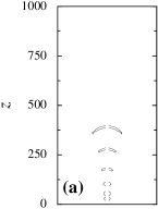
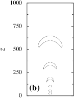
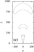
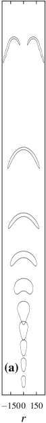
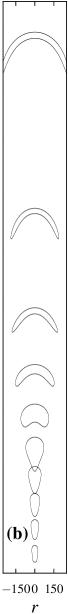
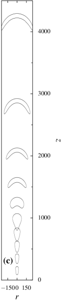
Figure 2: Evolution of streamers in a field of $\mathcal{E}=100$ kV/cm $p/p_{0}$ (left column) and in a field of $\mathcal{E}=40$ kV/cm $p/p_{0}$ (other three columns). Plotted is the contour of the half-maximum of the space charge at different times. The time interval between two consecutive snapshots is $\Delta t=150$ ps / $(p/p_{0})$ for the high field and $\Delta t=2400$ ps / $(p/p_{0})$ for the low field. Lengths are measured in units of $2.3$ $\mu$m / $(p/p_{0})$. Shown are streamers (a) without photoionization, (b) in air at atmospheric pressure, and (c) at low pressures ($p\ll 60\,\mathrm{Torr}$). Note that the computational domain is larger than the plotted area.

Simulation results and conclusions. Some simulation results for the evolution of the streamer head in different fields and pressures are shown in Fig. 2. Let us focus first on the high field regime which is represented in the left column of the figure; there it can be seen that during the first three to four time steps, the streamer development is barely affected by photoionization processes. However, eventually a new phase sets in where the streamer accelerates significantly. This acceleration is the stronger, the higher the relative contribution of photoionization, i.e., the lower the pressure. On the other hand, field enhancement is much weaker: it increases by $\sim 400\%$ without photoionization and only by $\sim 60\%$ in the low pressure case.

In the lower field case, a very different behavior is seen: photoionization hardly changes the streamer velocity. However, now it does suppress streamer branching as also found in Ref. Liu and Pasko, 2004. This can directly be related to the fact that photoionization makes particle distributions smoother, and that a smoother space charge layer is less susceptable to a Laplacian instability Arrayás et al. (2002); Ebert et al. (2006).

This smoothening dynamics can be made more precise by plotting the logarithm of the electron density along the symmetry axis of the streamer in Fig. 3. Photoionization creates a smoothly decaying density tail ahead of the ionization front that initially is not visible on a linear (non-logarithmic) scale. The point where the steep density decrease crosses over a smoother photoionization induced decay, moves toward higher density levels with time. For low fields (Fig. 3, below) up to the time when the streamer without photoionization branches, the large density levels visible in Fig. 2, move essentially with the same velocity. This is different in the high field case (Fig. 3, above): there the photon created leading edge eventually dominates the complete decay of the electron density and pulls the ionization front to much higher velocities Ebert and van Saarloos (2000).

Figure 3: Evolution of the logarithmic electron density on the streamer axis at pressure $p\ll 60\,\mathrm{Torr}$ (solid lines) and without photoionization (dashed lines) in the high field (above), corresponding to columns 2 and 4 in Fig. 2, and low field (below), which corresponds to the upper and lower plots in the left column of Fig. 2.

Acknowledgements: A.L. was supported by the Dutch STW project CTF.6501, C.M. by the FOM/EW Computational Science program, both make part of the Netherlands Organization for Scientific Research NWO.

References

- Raizer (1991) Y. Raizer, Gas Discharge Physics (Springer, Berlin, 1991).
- van Veldhuizen (2000) E. van Veldhuizen, Electrical Discharges for Environmental Purposes: Fundamentals and Applications (Nova Science Publishers, 2000).
- Gerken et al. (2000) E. Gerken, U. Inan, and C. Barrington-Leigh, Geophys. Res. Lett. 27, 2637 (2000).
- Williams (2006) E. Williams, Plasma Sour. Sci. Techn. 15, S91 (2006).
- Liu and Pasko (2004) N. Liu and V. Pasko, J. Geophys. Res. 109, A04301 (2004), J. Phys. D: App. Phys. 39, 327 (2006).
- Zheleznyak et al. (1982) M. Zheleznyak, A. Mnatsakanyan, and S. Sizykh, High Temp. 20, 357 (1982).
- Ebert et al. (2006) U. Ebert et al., Plasma Sour. Sci. Techn. 15, S118 (2006).
- Montijn et al. (2006a) C. Montijn, W. Hundsdorfer, and U. Ebert, J. Comp. Phys. (2006a), (in press), Phys. Rev. E 73 065401, (2006b).
- Legler (1963) W. Legler, Z. Phys. 169 (1963).
- Naidis (2006) G. V. Naidis, Plasma Sour. Sci. Techn. 15, 253 (2006).
- Kulikovsky (2000) A. Kulikovsky, J. Phys. D: Appl. Phys. 33, 1514 (2000).
- Sweet (1977) R. A. Sweet, SIAM J. Numer. Anal. 14, 706 (1977).
- Wackers (2005) J. Wackers, J. Comp. Appl. Math. 180, 1 (2005).
- Penney and Hummert (1970) G. Penney and G. Hummert, J. Appl. Phys 41, 572 (1970).
- Pancheshnyi (2005) S. Pancheshnyi, Plasma Sour. Sci. Techn. 14, 645 (2005).
- Arrayás et al. (2002) M. Arrayás, U. Ebert, and W. Hundsdorfer, Phys. Rev. Lett. 88, 174502 (2002).
- Ebert and van Saarloos (2000) U. Ebert and W. van Saarloos, Physica D 146, 1 (2000).