Bubbles and Filaments: Stirring a Cahn–Hilliard Fluid

Abstract

The advective Cahn–Hilliard equation describes the competing processes of stirring and separation in a two-phase fluid. Intuition suggests that bubbles will form on a certain scale, and previous studies of Cahn–Hilliard dynamics seem to suggest the presence of one dominant length scale. However, the Cahn–Hilliard phase-separation mechanism contains a hyperdiffusion term and we show that, by stirring the mixture at a sufficiently large amplitude, we excite the diffusion and overwhelm the segregation to create a homogeneous liquid. At intermediate amplitudes we see regions of bubbles coexisting with regions of hyperdiffusive filaments. Thus, the problem possesses two dominant length scales, associated with the bubbles and filaments. For simplicity, we use use a chaotic flow that mimics turbulent stirring at large Prandtl number. We compare our results with the case of variable mobility, in which growth of bubble size is dominated by interfacial rather than bulk effects, and find qualitatively similar results.

I Introduction

In a seminal paper, Cahn and Hilliard CH_orig introduced their eponymous equation to model the dynamics of phase separation. They pictured a binary alloy in a mixed state, cooling below a critical temperature. This state is unstable to small perturbations so that fluctuations cause the alloy to separate into bubbles (or domains) rich in one material or the other. A small transition layer separates the bubbles. Because the evolution of the concentration field is an order parameter equation, this description is completely general. Thus, by coupling the phase-separation model to fluid equations, one has a broad description of binary fluid flow encompassing polymers, immiscible binary fluids with interfacial tension, and glasses.

In industrial applications, the components of a binary mixture often need to be mixed in a homogeneous state. In that case, the coarsening tendency of multiphase fluids is undesirable. In this paper we will examine how a stirring flow affects this mixing process. We are interested in stirring not just to limit bubble growth, as is often effected with shear flows, but to break up the bubbles into a homogeneous mixture.

We first outline previous work for three increasing levels of complexity: Cahn–Hilliard (CH) in the absence of flow, passive CH with flow, and active CH with flow. Our focus in this paper will be on the passive case.

Cahn–Hilliard fluids without flow: There is a substantial literature that treats of the CH equation without flow. For a review, see Bray_advphys . The main physical feature of this simpler model is the existence of a single length scale (the bubble or domain size) such that quantities of interest (e.g., the correlation function) are self-similar under this scale. This length grows in time as $t^{1/3}$, a result seen in many numerical simulations (see, for example, Zhu et al. Zhu_numerics ). Of mathematical interest are the existence of a Lyapunov functional, and hence of a bounded solution Elliott_Zheng , and the failure of the maximum principle owing to fourth-order derivatives in the equation for the concentration field Gajewski_nonlocal ; Elliott_varmob .

Passive Cahn–Hilliard fluids: Given an externally imposed flow (e.g., a shear flow, turbulence, or a stirring motion), we have a passive tracer equation for a Cahn–Hilliard (CH) fluid. In the same way that one invokes the mixing of coffee and cream to picture the mechanisms at work in the advection-diffusion equation, this is the chef’s problem of how to mix olive oil and soy sauce by stirring.

There have been several studies of the (active and passive) shear-driven CH fluid shear_Shou ; shear_Berthier . In these studies, it is claimed that domain elongation persists in a direction that asymptotically aligns with the flow direction, while domain formation is arrested in a direction perpendicular to this axis. This seems to be confirmed in the experiments of Hashimoto Hashimoto , although these results could be due to finite-size effects shear_Bray , in which the arrest of domain growth is due to the limitation of the boundary on domain size. Of interest is the existence or otherwise of an arrest scale and the dependence of this scale on the system parameters.

A more effective form of stirring involves chaotic flows, in which neighboring particle trajectories separate exponentially in time, leading to chaotic advection Aref1984 . The average rate of separation is the Lyapunov exponent, positive for such a flow Eckmann1985 ; WigginsIntroDynSys . One may also regard this exponent as the average rate of strain of the flow. By imposing a chaotic flow on the CH fluid, finite-size effects are easily overcome. This is because the shear direction changes in time, so that domain elongtation in one particular direction, leading to an eventual steady state in which domains touch many walls, is no longer possible. Berthier et al. chaos_Berthier investigated the passive stirring of the CH fluid and observed a coarsening arrest arising from a dynamical balance of surface tension and advection. The stirring by the chaotic flow destroys large-scale structures, and this is balanced by the domain-forming tendency of the CH equation. A balancing scale is identified with the equilibrium domain size.

The importance of exponential stretching is amplified by the results of Lacasta et al. Sancho , in which a passive turbulent flow endowed with a tunable amplitude, correlation length, and correlation time, causes both arrest and indefinite growth, in different limits. We explain this heuristically as follows: In one limit of turbulent flow (small Prantdl number), the correlation length of the turbulent velocity field is small compared to the typical bubble size, fluid particles diffuse Taylor1921 , and bubble radii evolve as ${dR_{b}^{2}}/dt=2\kappa_{\mathrm{eff}}+\text{[Cahn--Hilliard contribution]}$, where $R_{b}$ is the bubble radius and $\kappa_{\mathrm{eff}}$ is the effective tracer diffusivity. Because $\kappa_{\mathrm{eff}}>0$, the presence of diffusion fails to arrest bubble growth. In the limit of large Prantdl number however, the the correlation length is large and the velocity field gives rise to exponential separation of trajectories, so that the radius equation is ${dR_{b}^{2}}/{dt}=-2\lambda R_{b}^{2}+\text{[Cahn--Hilliard contribution]}$, where $\lambda$ is the average rate of strain, or Lyapunov exponent, of the flow. Thus, the exponential stretching due to stirring balances the bubble growth. Lacasta et al. Sancho identify a critical correlation length above which coarsening arrest always takes place, no matter how small the stirring amplitude. Since chaotic flows typically exhibit long-range correlations, we expect they will always produce coarsening arrest.

Active Cahn–Hilliard fluids: At the highest level of complexity, one considers the reaction of the mixture on the flow by coupling the CH equation to the Navier–Stokes equations. For a derivation of the Navier–Stokes Cahn–Hilliard equations, see LowenTrus . In experiments involving turbulent binary fluids near the critical temperature, it is found that a turbulent flow suppresses phase separation and homogenizes the fluid Pine1984 ; Chan1987 . However, by cooling the fluid further and maintaining the same level of forcing, phase separation is achieved. This result is limited to near-critical fluids, although it does suggest the possibility of homogenization by stirring in other contexts.

The most recent work on the CH fluid (Berti et al., Berti_goodstuff ) focusses on the active CH tracer. They couple the CH concentration field to an externally forced velocity field and observe coarsening arrest independently of finite-size effects. They identify a balance of local shears and surface tension as the mechanism for coarsening arrest. Thus, the chaotic advection discussed above is a sufficient condition for coarsening arrest, but not a necessary one since shear will suffice. Of interest again is the dependence of the arrest scale on the mean rate of shear.

With this literature in mind, we study the case of a chaotic flow coupled passively to the CH equation. Our ultimate focus will be on the breakup of bubbles by stirring, and not just coarsening arrest. We believe this aspect of CH flow deserves a further and more complete study, as it is a regime of particular relevance to industry, for example, in droplet breakup or in the mixing of polymers Aarts .

Berthier et al. chaos_Berthier used an alternating sine flow to study coarsening arrest. Because of its simplicity, the sine flow is a popular testbed for studying chaotic mixing lattice_PH2 ; Antonsen1996 ; Neufeld_filaments ; lattice_PH1 ; Thiffeault2004 . In contrast to Berthier et al. chaos_Berthier , we use a sine flow where the phase is randomized at each period (see Section III), leading to a flow that has a positive Lyapunov exponent at all stirring amplitudes and for all initial conditions. This avoids the coexistence of regular and chaotic regions, which would lead to inhomeogeneous mixing characteristics over the domain of the problem. Because of its uniform stirring, the random-phase sine flow is often used as a proxy for turbulent stirring at high Prandtl number, but at much lower computational cost. Using this flow, we study coarsening arrest, as in previous papers chaos_Berthier ; Berti_goodstuff . However, we shall also use it to study mixing due to the stirring and the hyperdiffusion of the CH dynamics. Under this additional process the scaling hypothesis that characterizes the dynamics of bubble formation, namely that there is one dominant length scale Bray_advphys ; Berti_goodstuff , breaks down.

Following studies made Batchelor on the advection-diffusion equation Batchelor1959 and by Neufeld on reaction-diffusion equations Neufeld_filaments , we introduce a one-dimensional equation in order to model the formation of bubbles and the influence of advection and hyperdiffusion on the bubble size. This will lead to an understanding of the mechanism by which the bubbles are broken up and hyperdiffusion is becomes dominant.

The paper is laid out in the following way. In Section II we introduce the CH equation with advection and discuss its scaling laws. In Section III we present some numerical simulations of the two-dimensional equations, with and without flow, and confirm the scaling laws. In Section IV we make use of the one-dimensional CH equation coupled to a straining flow to understand the results from the two-dimensional simulations. In Section V we investigate numerically the two-dimensional CH equation with variable mobility.

II The Model Equation and its Scaling Laws

In this section we introduce the advective Cahn–Hilliard equation in $n$ dimensions. We then discuss the notion of dynamical equilibrium for the CH equation without flow in terms of the structure function. Finally, we study the length scales that arise in the presence of flow.

Let $c\left(\bm{x},t\right)$ be the conserved order parameter of the problem and let $\bm{v}\left(\bm{x},t\right)$ be an externally imposed two-dimensional incompressible flow, $\nabla\cdot\bm{v}=0$. The advective Cahn–Hilliard equation describes the phase separation dynamics of the field $c\left(\bm{x},t\right)$ in the presence of flow,

$$\frac{\partial c}{\partial t}+\bm{v}\cdot\nabla c=D\nabla^{2}\left(f_{0}^{\prime}\left(c\right)-\gamma\nabla^{2}c\right),$$ (1a)

$$f_{0}\left(c\right)=\tfrac{1}{4}\left(c^{2}-1\right)^{2}.$$ (1b)

This equation characterizes the stirring of a phase-separating binary liquid. Here $D$ is the (constant) mobility, which governs the rate of phase separation, and $\gamma$ is a hyperdiffusion coefficient. The fourth-order hyperdiffusion term in Eq. (1) has a mollifying effect that prevents the blow up of gradients. By identifying a chemical potential $\mu=f_{0}^{\prime}\left(c\right)-\gamma\nabla^{2}c$, Eq. (1) is recast as

$$\frac{\partial c}{\partial t}+\bm{v}\cdot\nabla c=D\nabla^{2}\mu\,.$$ (2)

The form of Eqs. (1) and (2) guarantees that the total concentration is conserved in the sense that $d/{dt}\int_{V}c\left(\bm{x},t\right)d^{n}x=0+\text{[boundary terms]}$. We let $V$ denote the problem domain as well as the system volume.

The CH equation without flow exhibits dynamical equilibrium in the following sense. Starting from a concentration field fluctuating around the unstable equilibrium $c\left(\bm{x},t\right)=0$, the late-time concentration field has properties that are time-independent when lengths are measured in units of typical bubble size $R_{\mathrm{b}}$. Such properties include the structure function Toral_scaling which we introduce below.

A measure of the correlation of concentration between neighbouring points, given in Fourier space, is the following:

$$S\left(\bm{k},t\right)=\frac{1}{V}\int_{V}d^{n}x\int_{V}d^{n}x^{\prime}e^{-i\bm{k}\cdot\bm{x}}\left[c\left(\bm{x}+\bm{x^{\prime}}\right)c\left(\bm{x}\right)-\langle c\rangle^{2}\right],$$ (3)

where angle brackets denote the spatial average. We normalize this function and compute its spherical average to obtain the structure function

$$s\left(k,t\right)=\frac{1}{\left(2\pi\right)^{n}}\frac{\tilde{S}\left(k,t\right)}{\langle c^{2}\rangle-\langle c\rangle^{2}}.$$ (4)

The spherical average $\tilde{\phi}\left(k\right)$ any function $\phi\left(\bm{k}\right)$ is defined as

$$\tilde{\phi}\left(k\right)=\frac{1}{\Omega_{n}}\int d\Omega_{n}\phi\left(\bm{k}\right),$$ (5)

where $d\Omega_{n}$ is the element of solid angle in $n$ dimensions and $\Omega_{n}$ is its integral. Thus $\tilde{c}_{k}$ is the spherical average of the Fourier coefficient $c_{\bm{k}}$. For a symmetric binary fluid $\langle c\rangle=0$, the structure function is simply the spherically averaged power spectrum:

$$s\left(k,t\right)=\frac{1}{\left(2\pi\right)^{n}}\frac{\left|\tilde{c}_{k}\right|^{2}}{\langle c^{2}\rangle},\qquad\text{for }\langle c\rangle=0.$$ (6)

The dominant length scale is identified with the reciprocal of the most important $k$-value, defined as the first moment of the distribution $s\left(k,t\right)$,

$$k_{1}=\frac{\int_{0}^{\infty}ks\left(k,t\right)dk}{\int_{0}^{\infty}s\left(k,t\right)dk}.$$ (7)

Since the system we study is isotropic except on scales comparable to the size of the problem domain, this length scale is is a measure of scale size in each spatial direction. That is, we have lost no information in performing the spherical average in Eq. (4). This length scale is in turn identified with the bubble size: $R_{\mathrm{b}}\propto 1/k_{1}$. In two-dimensional simulations ($n=2$) it is found Zhu_numerics ; Toral_scaling that while $k_{1}$ and $s\left(k,t\right)$ depend on time, $k_{1}^{n}s\left(k/k_{1},t\right)$ is a time-independent function with a single sharp maximum, confirming that the system is in dynamical equilibrium and that a dominant scale exists. Indeed, the growth law $R_{\mathrm{b}}\sim t^{1/3}$ is obtained, in agreement with the evaporation-condensation picture of phase separation proposed by Lifshitz and Slyozov (LS exponent) LS .

We present some simple scaling arguments to reproduce the $t^{1/3}$ scaling law and to illuminate the effect of flow. For $\bm{v}=\bm{0}$, the equilibrium solution of Eq. (1) is $c\approx\pm 1$ in domains, with small transition regions of width $\sqrt{\gamma}$ in between. Across these transition regions, it can be shown LowenTrus that

$$\mu=-{\Gamma\kappa}/2,$$

where

$$\Gamma=\sqrt{{8\gamma}/9}$$ (8)

is the surface tension and $\kappa$ is the radius of curvature. Thus, if $R_{\mathrm{b}}$ is a typical bubble size, that is, a length over which $c$ is constant, the chemical potential associated with the bubble is

$$\delta\mu\sim\Gamma/R_{\mathrm{b}}.$$ (9)

Balancing terms in Eq. (2), it follows that the time $t$ required for a bubble to grow to a size $R_{\mathrm{b}}$ is $1/t\sim{\Gamma D}/{R_{\mathrm{b}}^{3}}$, implying the LS growth law $R_{\mathrm{b}}\sim\left(\Gamma Dt\right)^{1/3}$.

Now the CH free energy $F[c]$ is the system energy owing to the presence of bubbles:

$$F[c]=\int_{V}d^{n}x\left[\tfrac{1}{4}\left(c^{2}-1\right)^{2}+\tfrac{1}{2}{\gamma}\left|\nabla c\right|^{2}\right].$$ (10)

The surface tension $\Gamma$ is the free energy per unit area. A bubble carries free energy $\Gamma R_{\mathrm{b}}^{n-1}$, where prefactors due to angular integration are omitted. The total free energy $F\left[c\right]$ in the motionless case is then $\Gamma R_{\mathrm{b}}^{n-1}\times N_{\mathrm{b}}$, where $N_{\mathrm{b}}$ is the total number of bubbles. Because the system is isotropic and because there is a well-defined bubble size, we estimate $N_{\mathrm{b}}$ by $V/{R_{\mathrm{b}}^{n}}$. The free energy then has the scale dependence $F/V\sim\Gamma/R_{\mathrm{b}}$, and using the growth law for the length $R_{\mathrm{b}}$ we obtain the asymptotic free energy relation

$$\frac{F}{V}\sim\left(\frac{\Gamma^{2}}{D}\right)^{1/3}t^{-1/3}.$$ (11)

By introducing the tracer variance

$$\sigma^{2}=\langle c^{2}\rangle-\langle c\rangle^{2}$$ (12)

and restricting to a symmetric mixture $\langle c\rangle=0$, we may identify $\sigma^{2}\simeq V_{\mathrm{b}}/V$, where $V_{\mathrm{b}}=N_{\mathrm{b}}R_{\mathrm{b}}^{n}$ is the volume occupied by bubbles. Since $F=\Gamma R_{\mathrm{b}}^{n-1}N_{\mathrm{b}}$, it follows that

$$R_{\mathrm{b}}\sim\sigma^{2}/F.$$ (13)

We shall verify these results in Section III. Equation (13) will provide a useful measure of bubble size when a flow is imposed, since no assumption is made about the number of bubbles per unit volume. In a dynamical scaling regime, the length scales calculated from these energy considerations must agree with that computed from the first moment of the structure function, since there is only one length scale in such a regime Furukawa_scales .

Stirring a CH fluid introduces new length scales. The flow will alter the sharp power spectrum found above and so it may not be possible to extract definite scales from experiments or numerical simulations. We might expect further ambiguity of scales during a regime change (crossover), for example, as the bubbles are broken up and diffusion takes over. Nevertheless, for a given flow it is possible to construct length scales from the system parameters. We shall impose a flow $\bm{v}\left(\bm{x},t\right)$ that is chaotic in the sense that nearby particle trajectories separate exponentially in time at a mean rate given by the Lyapunov exponent.

If the advection term and the surface tension term have the same order of magnitude in a chaotic flow, by balancing the terms $\bm{v}\cdot\nabla c$ and $D\nabla^{2}\mu$ we obtain a scale

$$R_{\mathrm{st}}=\left(\Gamma D/\lambda\right)^{1/3},$$ (14)

where $\lambda$ is the Lyapunov exponent of the flow. Because the term $\bm{v}\cdot\nabla c$ gives an exponential amplification of gradients, the balance of segregation and hyperdiffusion in the term $\mu=f_{0}^{\prime}\left(c\right)-\gamma\nabla^{2}c$ may be broken and hyperdiffusion may overcome segregration. This will happen on a scale $R_{\mathrm{diff}}$ given by the balance of the terms $\bm{v}\cdot\nabla c$ and $\gamma\nabla^{4}c$,

$$R_{\mathrm{diff}}=\left({\gamma D}/\lambda\right)^{1/4}.$$ (15)

In this regime, we expect mixing owing to the presence of the advection and the (hyper) diffusion. Using Eqs. (8), (14) and (15), the crossover between the bubbly and the diffusive regimes takes place when $\lambda\simeq D/\gamma$. In the following sections we shall examine these scales and look for this crossover between bubbles and filaments, the latter being characteristic of mixing by advection-diffusion.

III Numerical Solution of the Two-Dimensional Problem

In order to run simulations at high resolution, we specialize to two dimensions. We solve Eq. (1) with and without flow to investigate the scaling laws presented in the previous section.

Equation (1) is integrated by an operator splitting technique, in which a specialized advective step followed by a phase-separation step are performed at each iteration. The phase separation step is the semi-implicit spectral algorithm proposed by Zhu et al. Zhu_numerics for the case without flow. The semi-implicitness of the algorithm enables us to use a reasonably large time step. We use the following velocity field, defined on a $\left(2\pi\right)\times\left(2\pi\right)$ grid of $512^{2}$ points with periodic boundary conditions,

$$\begin{split}v_{x}\left(x,y,t\right)&=\alpha\sin\left(y+\phi_{n}\right),\qquad v_{y}=0,\qquad n\tau\leq t<\left(n+\tfrac{1}{2}\right)\tau,\\ v_{y}\left(x,y,t\right)&=\alpha\sin\left(x+\psi_{n}\right),\qquad v_{x}=0,\qquad\left(n+\tfrac{1}{2}\right)\tau\leq t<\left(n+1\right)\tau,\end{split}$$ (16)

where $\phi_{n}$ and $\psi_{n}$ are phases that are randomized once during each flow period $\tau$ and the integer $n$ labels the period. We set $\tau=1$ and work in units where time is the number of periods. We use Pierrehumbert’s lattice method for advection lattice_PH1 ; lattice_PH2 . With the problem defined on a discrete grid, this method is exact for the advection step. Using standard techniques Eckmann1985 ; WigginsIntroDynSys , we compute the Lyapunov exponent numerically and find it is always positive and independent of initial conditions, as expected for this flow. For the parameter regime $\alpha\in\left[0,1\right]$ we find

$$\lambda\sim 0.118\phantom{l}\alpha^{2},\qquad\alpha\lesssim 1,$$ (17)

a result that we shall use in what follows. For sufficiently large $\alpha$, it is easy to show the exact asymptotic result

$$\lambda\sim\log\left(\tfrac{1}{4}\,{\alpha^{2}}\right),\qquad\alpha\gg 1.$$ (18)

Furthermore, the correlation length for the velocity is of order of the box size, which is the largest scale in the problem. Therefore, using the prediction of Lacasta et al. Sancho , we expect this velocity field to produce coarsening arrest even at very small stirring amplitudes.

We integrate Eq. (1) in the manner explained above. The initial conditions are chosen to represent the sudden cooling of the binary fluid: Above a certain temperature $T_{\mathrm{c}}$ the homogeneous state $c=0$ is stable, while below this temperature the mixture free energy changes character to become $\tfrac{1}{4}\left(c^{2}-1\right)^{2}$, which makes the homogeneous state unstable. Thus, at temperatures $T>T_{\mathrm{c}}$, $c\left(\bm{x}\right)=0+\text{[fluctuations]}$, and the sudden cooling of the system below $T_{\mathrm{c}}$

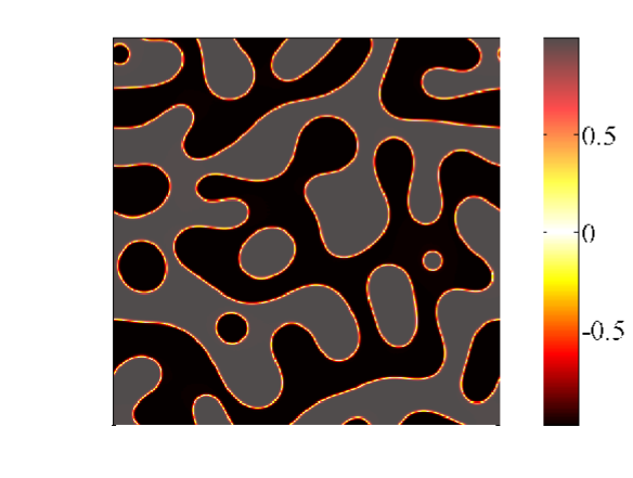
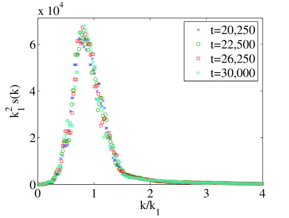
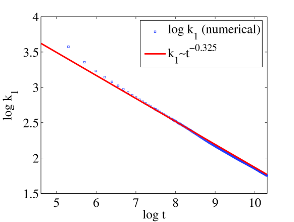
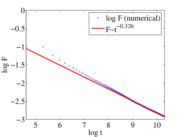
Figure 1: (a) Concentration, at $t=30,000$; (b) Structure function $k_{1}^{2}s\left(k/k_{1},t\right)$ in the scaling regime $t\geq 20,000$; (c) Time dependence of $k_{1}$, with power law exponent close to the LS exponent $1/3$; (d) Free energy, $F$, exhibiting the time dependence $F\sim t^{-0.326}$, close to the LS exponent.

leaves the system in this state. In order for the CH equation without thermal noise (1) to describe the evolution of these initial conditions, the cooling we have imposed must take the system to $T=0$. Thus, we are working in the so-called deep-quench limit. With the initial conditions $c\left(\bm{x},0\right)=0+\text{[fluctuations]}$, both components of the fluid are present in equal amounts and the spatial average of the concentration field is zero.

Although the case without flow has been investigated before Zhu_numerics ; Toral_scaling , we reproduce it for two reasons. First, it serves as a validation of our algorithm. Second, we shall confirm the free energy laws (11) and (13) which to our knowledge have not been examined before. Finding an appropriate measure of bubble growth will be important for understanding the behavior of the bubbles when we introduce stirring.

The results of these simulations are presented in Fig. 1. The scaling function $k_{1}^{2}s\left(k/k_{1},t\right)$ is approximately time-independent for $t>20,000$ as evidenced by Fig. 1(b), implying that the scaling exponents for $k_{1}$ and $F$ are to be extracted from the late-time data with $t>20,000$. For $t>30,000$ finite-size effects spoil the scaling laws. Thus while the scaling exponents are extracted from a small window, the fit is good and this suggests that the power laws obtained give the true time-dependence of $k_{1}$ and $F$ at late times. In this way we recover the dynamical scaling regime in which $k_{1}^{2}s\left(k/k_{1},t\right)$ is time-independent, in addition to the decay law $k_{1}\sim t^{-1/3}$ Zhu_numerics . Running the simulation repeatedly for an ensemble of random initial conditions improves the accuracy of the exponent. Furthermore we obtain the energy laws $F\sim c_{1}t^{-1/3}$, and $1-\sigma^{2}\sim c_{2}t^{-1/3}$. Thus,

$$\frac{\sigma^{2}}{F}=\frac{1-c_{2}t^{-1/3}}{c_{1}t^{-1/3}}\sim\frac{1}{c_{1}}t^{1/3},\qquad\text{for }t\gg 1$$ (19)

so that $\sigma^{2}/F$, $1/F$ and $1/k_{1}$ all grow as $t^{1/3}$ and hence provide identical measures of scale growth, in agreement with the classical assumption that there is a unique length scale in the problem Bray_advphys ; Zhu_numerics .

We investigate the stirred case in a similar manner and obtain the results below, after $t=30,000$ time steps. In order to ensure that we are in a steady state, we study the inverse lengths $F$ and $k_{1}$ and the tracer variance $\sigma^{2}$ (see Eq. (12)) which measures the homogeneity of the concentration ($\sigma^{2}=0$ for a homogeneous mixture) lattice_PH1 ; lattice_PH2 . These quantities are time-dependent and have the property that after some transience, they fluctuate around a mean value, without secular trend. This can be seen in Fig. 2.

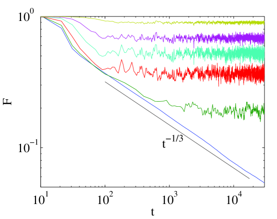
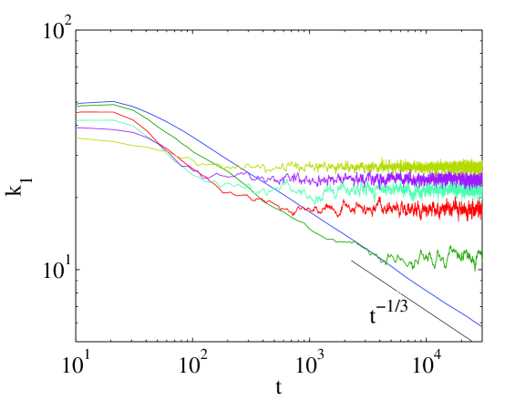
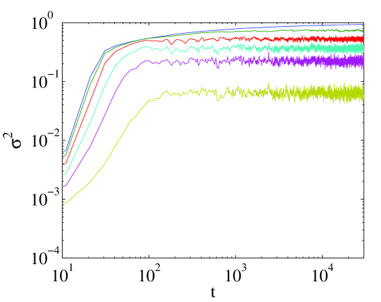
Figure 2: (a) $F$ vs $t$ for (from bottom) $\alpha=0,0.1,0.3,0.5,0.7,1.0$; (b) $k_{1}$ vs $t$ for the same values of $\alpha$; (c) Tracer variance $\sigma^{2}$ for (from bottom) $\alpha=1.0,0.7,0.5,0.3,0.1,0$.

In Fig. 3, for $\alpha=0.1$, the concentration field at late time looks

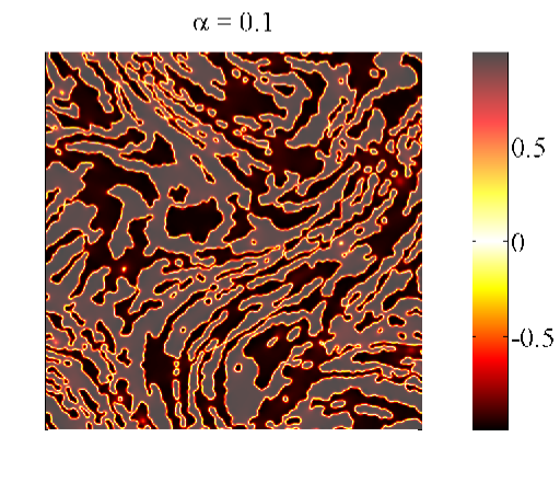
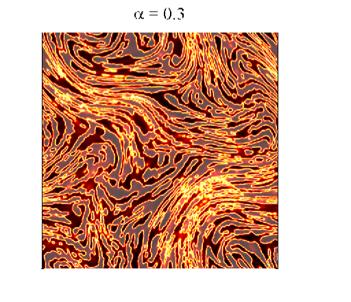
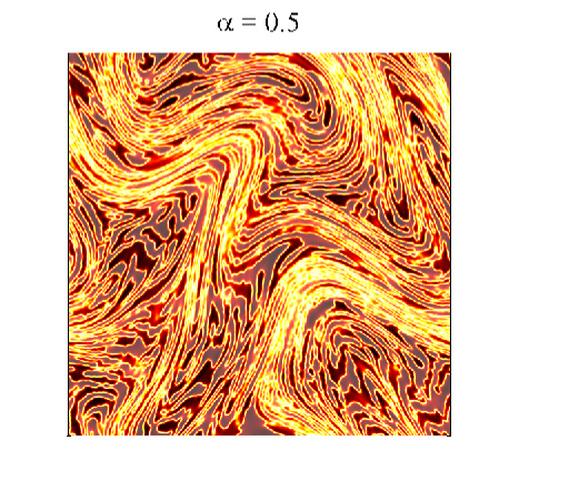
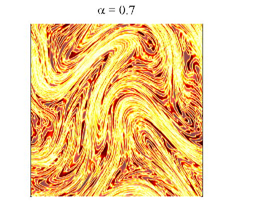
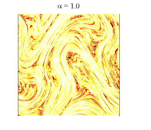
Figure 3: The steady-state concentration field after $t=30,000$ timesteps, for various stirring amplitudes $\alpha$.

similar to that for $\alpha=0$. This is because for small $\alpha$, the effect of advection is diffusive, with small movements of particles giving rise to bubbles with jagged boundaries, but no breakup. The PDFs of the concentration for $\alpha\in[0,0.01,...,0.2]$ have the same structure. Nevertheless, it is clear from Fig. 2(b) that coarsening arrest takes place for $\alpha=[0.01,...,0.2]$, in contrast to $\alpha=0$. As $\alpha$ increases, the bubbles become less and less evident. For large $\alpha$, we see regions containing filaments of similar concentration. After a period of transience, the free energy $F$, the mean wavenumber $k_{1}$ and the variance $\sigma^{2}$ fluctuate around mean values, confirming the existence of the steady state. The bubble size is extracted from the quantity $\overline{\sigma^{2}/F}$, where the overbar denotes a time average over the fluctuations. We investigate how the mean lengths scale with the Lyapunov exponent $\lambda$.

In Fig. 4 we see that for small $\lambda$ the proxy $\overline{\sigma^{2}/F}$ for bubble radius scales with the

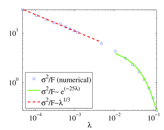
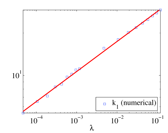
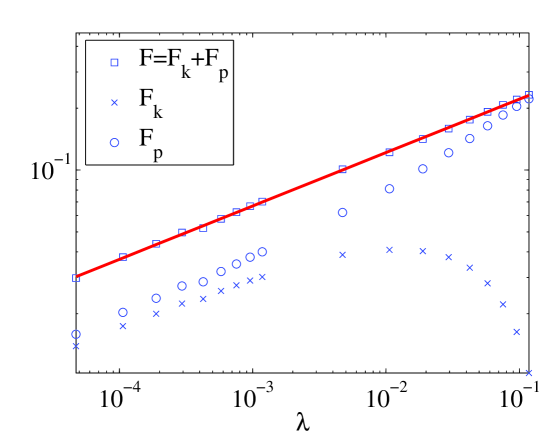
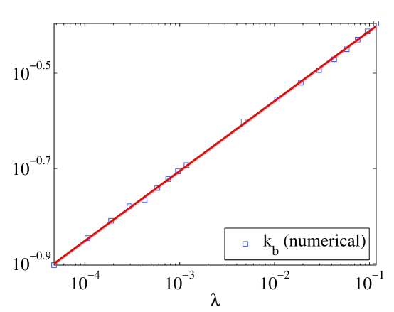
Figure 4: (a) The plot of $\log\big{(}\overline{\sigma^{2}/F}\big{)}$ against $\log\lambda$ suggests the scaling law $\overline{\sigma^{2}/F}\sim\lambda^{-1/3}$ for small stirring amplitudes while for large amplitudes this proxy for the bubble radius decays exponentially with increasing Lyapunov exponent. (b) Graph of $\log\overline{k_{1}}$ against $\log\lambda$, with approximate power law behavior $\overline{k_{1}}\sim\lambda^{0.21}$. The exponent is not the same over the entire range, however. (c) The graph of $\log\overline{F}$ exhibits a much cleaner power law behaviour $\overline{F}\sim\lambda^{0.26}$. (d) The Batchelor wavenumber $k_{b}=\big{[}{\langle\left|\nabla c\right|^{2}\rangle}/{\langle c^{2}\rangle}\big{]}^{1/2}$ also possesses a clear power law behaviour $\overline{k_{b}}\sim\lambda^{0.15}$.

LS exponent as $\lambda^{-1/3}$, suggesting an equilibrium bubble size on this scale. For larger $\lambda$, the hyperdiffusion breaks up these bubbles and mixes the fluid. This process leads to a faster than algebraic decay of bubble size, visible in the figure. Other measures of the bubble size, such as the mean wavenumber $\overline{k_{1}}$ or the quantity $1-\overline{\sigma^{2}}$ do not possess a clear scaling law. For example, in Fig. 4(b) we plot $\log\overline{k_{1}}$ against $\log\lambda$. The exponent changes over the three decades of data, indicating that the wavenumber $\overline{k_{1}}$ does not have a clear scaling law with the Lyapunov exponent $\lambda$. However, the dependence of the time-averaged free energy on the Lyapunov exponent has the power law behavior $\overline{F}\sim\lambda^{0.26}$ over three decades, suggesting a genuine power law relationship. The Batchelor wavenumber $k_{b}=[{\langle\left|\nabla c\right|^{2}\rangle}/{\langle c^{2}\rangle}]^{1/2}$ Batchelor1959 also possesses a clean power law over three decades.

Furukawa Furukawa_scales shows that in a situation of dynamical equilibrium characterized by a single length scale, the potential part of the free energy $F_{\mathrm{p}}=\tfrac{1}{4}\int d^{2}x\left(c^{2}-1\right)^{2}$ should be in equipartition with the kinetic part $F_{\mathrm{k}}=\tfrac{1}{2}\int d^{2}x\gamma\left|\nabla c\right|^{2}$. In Fig. 4 we see that this is not the case when the bubbles start to break up as the stirring is increased. This is an indication of a crossover between the bubbly regime and the well-mixed one in which the variance is reduced by stirring.

In Fig. 4 the breakdown in the power law relationship $\overline{\sigma^{2}/F}\sim\lambda^{-1/3}$ for large stirring amplitudes suggests the crossover between a bubbly regime and a diffusive one. Another way of seeing the transition between these regimes is to study the stationary probability distribution function (PDF) of the field $c\left(\bm{x},t\right)$. We show this in Fig. 5. For small

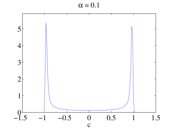
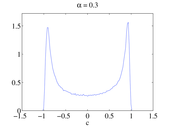
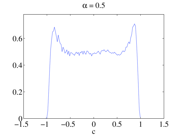
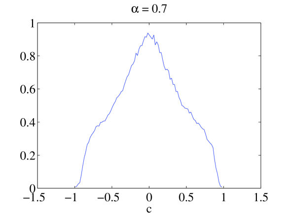
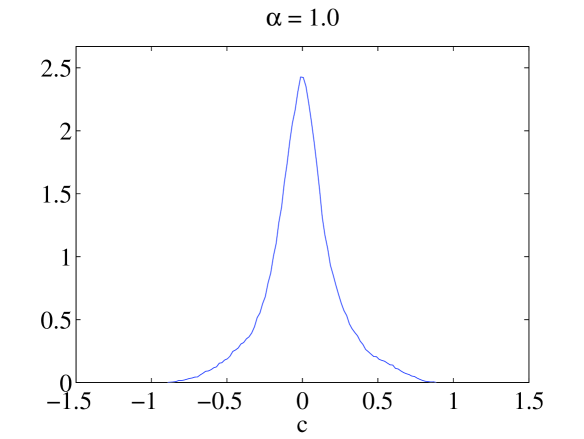
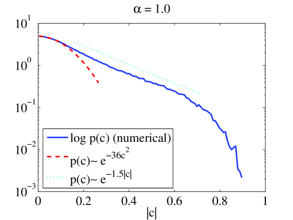
Figure 5: Normalized PDF of concentration in the steady state. (a), (b) Segregation-dominated flow ($\alpha=0.1,0.3$); (c), (d) Crossover to quasi-diffusive regime ($\alpha=0.5,0.7$); (e) Quasi-diffusive regime ($\alpha=1$); (f) Semilog plot of PDF for $\alpha=1.0$. Note Gaussian core and exponential decay down to the cutoff at $\left|c\right|\lesssim 1$.

values of $\alpha$ we note that the PDF has sharp peaks at $\pm 1$, indicating the effectiveness of phase separation at these stirring amplitudes. For $\alpha=1$ however, the PDF has a Gaussian core, indicating that genuine mixing by advection-hyperdiffusion is taking place. For intermediate values of $\alpha$ the PDF is a combination of these two different distributions of concentration.

IV A One-Dimensional Equilibrium Problem

Having observed the crossover between the bubbly and the well-mixed regimes, we study a one-dimensional model to shed further light on the process by which this occurs.

We examine the archetypal hyperbolic flow $\bm{v}=\left(-\lambda x,\lambda y\right)$, with strain rate $\lambda$. This flow tends to homogenize the concentration in the $y$-direction through stretching. At late times the problem then becomes one-dimensional,

$$\frac{\partial c}{\partial t}-\lambda x\frac{\partial c}{\partial x}=D\frac{\partial^{2}}{\partial x^{2}}\left(c^{3}-c\right)-\gamma D\frac{\partial^{4}c}{\partial x^{4}}.$$ (20)

Scaling lengths by $\sqrt{\gamma}$ and restricting to the steady case, Eq. (20) becomes

$$-\lambda\left(\frac{\gamma}{D}\right)x\frac{dc}{dx}=\frac{d^{2}}{dx^{2}}\left(c^{3}-c\right)-\frac{d^{4}c}{dx^{4}}.$$ (21)

This equation is invariant under the parity change $x\rightarrow-x$ and so we seek odd and even solutions. Thus we may restrict the solution to the half-line $\left[0,\infty\right)$. We choose the bubble boundary conditions $c\left(0\right)=1-\delta$, $c^{\prime}\left(0\right)=0$, $c\left(\infty\right)=-1$, $c^{\prime}\left(\infty\right)=0$. The addition of the small positive constant $\delta$ in the boundary conditions makes a bubble solution possible in the limit $\lambda\rightarrow 0$. In this limit, Eq. (21) reduces to

$$\frac{d^{2}}{dx^{2}}\left(c^{3}-c-\frac{d^{2}c}{dx^{2}}\right)=0$$ (22)

and using the boundary conditions, this simplifies further to

$$\tfrac{1}{2}\left(\frac{dc}{dx}\right)^{2}=\tfrac{1}{4}\left(c^{2}-1\right)^{2}+\left(-\tfrac{1}{2}\delta^{2}+\tfrac{1}{4}\delta^{3}\right)\left(c+1\right)\equiv\Phi\left(c\right),$$

where the function $\Phi\left(c\right)$ is positive definite on the interval $\left(-1,1-\delta\right)$. This equation has the implicit solution

$$x=\pm\frac{1}{\sqrt{2}}\int_{c\left(x\right)}^{1-\delta}\frac{dc}{\sqrt{\Phi\left(c\right)}}.$$

The bubble width is given by the unique zero of the function $c\left(x\right)$.

By measuring lengths in terms of the diffusion lengthscale $\left(\gamma D/\lambda\right)^{1/4}$, the large-$\lambda$ limit of Eq. (21) reduces to the advection-hyperdiffusion equation

$$x\frac{dc}{dx}=\frac{d^{4}c}{dx^{4}}.$$ (23)

Restoring the dimensional units, the general solution is given in terms of generalized Airy functions Polyanin_odes ,

$$c\left(x\right)=c\left(0\right)+\int_{0}^{x}dx^{\prime}\sum_{\nu=0}^{3}C_{\nu}v_{\nu}\left(x^{\prime}\right);\qquad v_{\nu}\left(x\right)=\epsilon_{\nu}\int_{0}^{\infty}\exp\left[\epsilon_{\nu}tx-\frac{t^{4}}{{4\lambda}/{\gamma D}}\right]dt,$$ (24)

where the constants $C_{\nu}$ sum to zero and the phases $\epsilon_{\nu}=\exp\left(i\pi\nu/2\right)$ are the fourth roots of unity. By inspection of the phases, we see that Eq. (23) lacks a bubble solution, although it does have a front solution. Since it is the segregation term which makes the existence of stationary bubbles possible, it is not surprising that no stationary bubble exists when this term is set to zero. Thus as $\lambda\rightarrow\infty$ the solution presented in Fig. 6 tends asymptotically to the function

$$\left(1-\delta\right)+\int_{0}^{x}\left[v_{1}\left(x^{\prime}\right)-\left(1-i\right)v_{2}\left(x^{\prime}\right)-iv_{3}\left(x^{\prime}\right)\right]dx^{\prime},$$

which diverges for $x\rightarrow-\infty$. Nevertheless, this solution on the restricted interval $\left[0,\infty\right)$ provides the correct parametric dependence of the length scale in the diffusive limit which suggests that we are justified in using it.

We mention briefly an alternative set of boundary conditions: let $c\left(\pm\infty\right)=\pm 1$ and $c^{\prime}\left(\pm\infty\right)=0$ (the $\delta$ term is unimportant now). This corresponds to a front. At small $\lambda$, this equation contains information about the width of the transition regions. Since in this limit, the front solution is independent of $\lambda$ and given by Eq. (22), there is no new information here. At large $\lambda$ this solution has the interpretation of being the transition layer between filaments, the width of the layer giving the width of the filament. In this limit, the solution is given by $\int_{0}^{x}\left[v_{1}\left(x^{\prime}\right)-v_{3}\left(x^{\prime}\right)\right]dx^{\prime}$. Thus, the front boundary conditions do not give any further information about the bubble / filament structures.

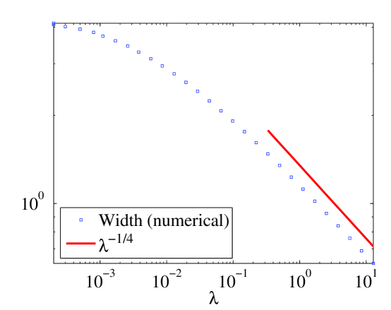
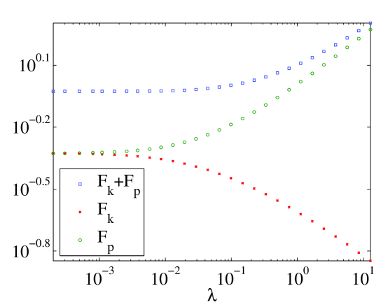
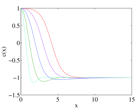
Figure 6: (a) Bubble width as a function of the strain rate $\lambda$; (b) Bubble free energy as a function of the strain rate; (c) Bubble profile for (from right to left) $\lambda=0.001,0.01,0.1,1,10$.

In Fig. 6 we provide the relation between the strain rate $\lambda$ and the bubble width and the bubble free energy. For small $\lambda$ these quantities depend only weakly on the strain rate while for large $\lambda$ the bubble width scales as $\lambda^{-1/4}$, in accordance with equation (15). It is not clear if the free energy also has this asymptotic dependence. For large $\lambda$, the free energy equipartition rule is broken, and the potential part dominates, in agreement with the results of Section III.

Moreover, Fig. 6 indicates that the bubble width decreases as the strain rate increases. Thus, the length scale over which $c$ is constant diminishes with increasing $\lambda$ so that for sufficiently large $\lambda$, the bubble size is less than or of the order of the transition region size. That is, $\left({\gamma D}/\lambda_{\mathrm{c}}\right)^{1/4}=\gamma^{1/2}$, so $\lambda_{\mathrm{c}}=D/\gamma$. On these scales, only diffusion is important and hence the tendency to form bubbles is overcome. Thus, the one-dimensional model explains at least qualitatively why the crossover from the bubbly to the diffusive regime occurs. This prediction for $\lambda_{c}$ is in agreement with the prediction in Section II and is in approximate agreement with the numerical simulations, where the crossover occurred at $\alpha\simeq 1$ ($\lambda\simeq 0.2$, $\tau D=\gamma$).

Finally we note that the concentration profile takes values $\left|c\right|>1$ in some places, a consequence of Eq. (21) lacking a maximum principle, in contrast (say) to the advection-diffusion equation. This is consistent with the numerical results of Section IV, where we find $\mathrm{max}_{\bm{x}\in V}\left|c\left(\bm{x},t\right)\right|>1$. As mentioned by Gajewski and Zacharias Gajewski_nonlocal , this super-abundance of one binary fluid element is unreasonable on physical grounds, pointing to a shortcoming in the advective CH model. However, we shall see in the next section that the qualitative features of this simple model and the more realistic variable-mobility model are in agreement, suggesting that the simpler model gives an adequate description of advective phase-separation dynamics.

V The Variable-Mobility Case

In order to gain further insight into the dependence of the bubble size on the Lifshitz-Slyozov and Lyapunov exponents, we study the variable-mobility Cahn–Hilliard equation Langer

$$\frac{\partial c}{\partial t}+\bm{v}\cdot\nabla c=\nabla\cdot\left[D\left(c\right)\nabla\mu\right],$$ (25)

where as before $\mu=f_{0}^{\prime}\left(c\right)-\gamma\nabla^{2}c$. By introducing this additional feature, we recover a system that, at least in the case without flow, has a solution $c\left(\bm{x},t\right)$ confined to the range $[-1,1]$ Elliott_varmob .

We specify the functional form of the mobility as

$$D\left(c\right)=D_{0}\left(1-\eta c^{2}\right),$$ (26)

fixing $\eta=1$. This modification corresponds to interface-driven coarsening because inside bubbles ($c=\pm 1$) the mobility is zero. For other values of $\eta$ we have a mixture of bulk- and interface-driven coarsening. This equation has been investigated by Bray and Emmott Bray_LSW for $\bm{v}=0$, in an evaporation-condensation picture. They show that the typical bubble size $R_{\mathrm{b}}\left(t\right)$ grows as $t^{1/4}$, a result limited to dimensions greater than two. Numerical simulations Zhu_numerics suggest that this growth law also holds in two dimensions. We couple the modified segregation dynamics to the sine flow.

For $\bm{v}=0$, we obtain the growth law for the scale $R_{\mathrm{b}}\equiv 1/k_{1}$, namely $R_{\mathrm{b}}\sim t^{0.264}$. The growth exponent is close to the value $1/4$ predicted by the LS theory. In addition, we obtain the free energy decay laws $F\sim t^{-0.267}$ again close to the LS value. Thus, as in the constant mobility case, a description of the length scales in the system can be given in terms of the bubble energy or in terms of $R_{\mathrm{b}}$, with identical results.

Because the variable mobility calculation is computationally slower, we perform the numerical experiments with flow at lower resolution. We do not anticipate that this will change the results, because in integrations of the constant-mobility equations at resolution $256^{2}$ the scaling exponents were unaffected. Switching on the chaotic flow, we observe a steady state characterized by fluctuation of the free energy, wave number $k_{1}$, and variance $\sigma^{2}$ around mean values. As in the constant mobility case, the time-averaged free energy and time-averaged Batchelor scale possess clear scaling laws,

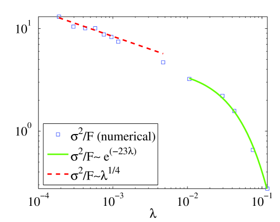
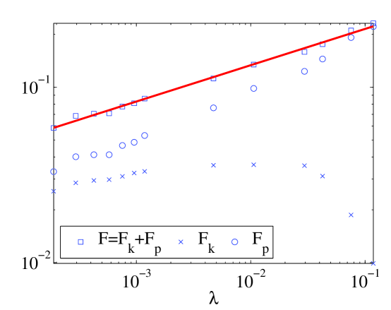
Figure 7: (a) The plot of $\log\big{(}\overline{\sigma^{2}/F}\big{)}$ against $\log\lambda$ suggests the scaling law $\overline{\sigma^{2}/F}\sim\lambda^{-1/4}$ for small stirring amplitudes, while for large amplitudes this proxy for the bubble radius decays exponentially with increasing Lyapunov exponent. (b) The graph of $\log\overline{F}$ exhibits power law behaviour $\overline{F}\sim\lambda^{0.21}$. The predominance of kinetic free energy over potential free energy at large $\lambda$ is visible.

while tthe mean wavenumber $\overline{k_{1}}$ does not. For small $\lambda$, the proxy for bubble radius $\overline{\sigma^{2}/F}$ scales approximately as $\lambda^{-1/4}$, suggesting a decay of bubble radius according to the LS exponent. Thus the analogous result of Section III is not fortuitous. For large $\lambda$ this quantity decays exponentially to zero at a rate (with respect to $\lambda$) close to that of the constant mobility system. In each case, the fit of the data is not as good as the constant mobility case, the computational error being larger here because we have run the simulations at resolution $256^{2}$. We present these results in Fig. 7.

The results are an exact replica of those for the constant mobility case. Thus, the arrest of bubble growth for small $\lambda$ is a genuine phenomenon whose behavior depends on the LS exponent of the corresponding unstirred dynamics. The mixing at large $\lambda$ is identical to that for which the mobility is constant. Thus, while the variable mobility model is more realistic than its constant-mobility counterpart, their properties with regard to mixing are the same.

VI Conclusions

We have shown how, in the presence of an external chaotic stirring, the coarsening dynamics of the Cahn–Hilliard equation are arrested and bubbles form on a particular length scale. The system reaches a steady state, characterized by the fluctuation of the free energy $F$, the variance $\sigma^{2}$, and the wavenumber $k_{1}$ around mean values. A measure of the typical bubble size is given by the time-average of $\sigma^{2}/F$. For sufficiently large stirring intensities, the bubbles diminish in prominence, to be replaced by filament structures. These are due to the combination of the advection and hyperdiffusion terms in the CH demixing mechanism. In this regime, the concentration tends to homogenize, so that the stirring stabilizes the previously unstable mixed state.

We have explained with a one-dimensional model how this transition arises and how the filament width in the homogeneous regime depends on the Lyapunov exponent of the chaotic flow. This latter investigation exhibits the super-abundance of one binary fluid element at a particular location in space, which we reject as unreasonable. In this result, we see how the lack of a maximum principle for the constant-mobility CH equation limits its physical relevance. In the case of no flow this difficulty was overcome by the addition of a variable mobility Elliott_varmob . However, the quasi-diffusive regime identified in our simulations is robust in the sense that it is present in both the constant and the more realistic variable mobility cases. We therefore expect to see this remixing phenomenon in real binary fluids.

References

- (1) J. W. Cahn and J. E. Hilliard, “Free energy of a nonuniform system. I. Interfacial energy,” J. Chem. Phys 28, 258 (1957).
- (2) A. J. Bray, “Theory of phase-ordering kinetics,” Adv. Phys. 43, 357 (1994).
- (3) J. Zhu, L. Q. Shen, J. Shen, V. Tikare, and A. Onuki, “Coarsening kinetics from a variable mobility Cahn–Hilliard equation: Application of a semi-implicit Fourier spectral method,” Phys. Rev. E 60, 3564 (1999).
- (4) C. M. Elliott and S. Zheng, “On the Cahn–Hilliard equation,” Arch. Rat. Mech. Anal. 96, 339 (1986).
- (5) H. Gajewski and K. Zacharias, “On a nonlocal phase separation model,” J. Math. Anal. Appl. 286, 11 (2003).
- (6) C. M. Elliott and H. Garcke, “The Cahn–Hilliard equation with degenerate mobility,” SIAM J. Math. Anal. 27, 403 (1996).
- (7) Z. Shou and A. Chakrabarti, “Ordering of viscous liquid mixtures under a steady shear flow,” Phys. Rev. E 61, R2200 (2000).
- (8) L. Berthier, “Phase separation in a homogeneous shear flow: Morphology, growth laws, and dynamic scaling,” Phys. Rev. E 63, 051503 (2001).
- (9) T. Hashimoto, K. Matsuzaka, and E. Moses, “String phase in phase-separating fluids under shear flow,” Phys. Rev. Lett. 74, 126 (1995).
- (10) A. J. Bray, “Coarsening dynamics of phase-separating systems,” Phil. Trans. R. Soc. Lond. 361, 781 (2003).
- (11) H. Aref, “Stirring by chaotic advection,” J. Fluid Mech. 143, 1 (1984).
- (12) J.-P. Eckmann and D. Ruelle, “Ergodic theory of chaos and strange attractors,” Rev. Mod. Phys. 57, 617 (1985).
- (13) S. Wiggins, Introduction to Applied Dynamical Systems and Chaos, 2nd ed. (Springer-Verlag, New York, 2003).
- (14) L. Berthier, J. L. Barrat, and J. Kurchan, “Phase separation in a chaotic flow,” Phys. Rev. Lett. 86, 2014 (2001).
- (15) A. M. Lacasta, J. M. Sancho, and F. Sagues, “Phase separation dynamics under stirring,” Phys. Rev. Lett. 75, 1791 (1995).
- (16) G. I. Taylor, “Diffusion by continuous movement,” Proc. London Math. Soc. 20, 196 (1921).
- (17) J. Lowengrub and L. Truskinowsky, “Quasi-incompressible Cahn–Hilliard fluids and topological transitions,” Proc. R. Soc. Lond. A 454, 2617 (1998).
- (18) D. J. Pine, N. Easwar, J. V. Maher, and W. I. Goldburg, “Turbulent suppression of spinodal decomposition,” Phys. Rev. A 29, 308 (1984).
- (19) C. K. Chan, W. I. Goldburg, and J. V. Maher, “Light-scattering study of a turbulent critical binary mixture near the critical point,” Phys. Rev. A 35, 1756 (1987).
- (20) S. Berti, G. Boffetta, M. Cencini, and A. Vulpiani, “Phase separation in a chaotic flow,” Phys. Rev. Lett. 95, 224501 (2005).
- (21) D. G. A. L. Aarts, R. P. A. Dullens, and H. Lekkerherker, “Interfacial dynamics in demixing systems with ultralow interfacial tension,” New J. Phys. 7, 14 (2005).
- (22) R. T. Pierrehumbert, “Tracer microstructure in the large-eddy dominated regime,” Chaos, Solitons and Fractals 4, 1091 (1994).
- (23) T. M. Antonsen, Jr., Z. Fan, E. Ott, and E. Garcia-Lopez, “The role of chaotic orbits in the determination of power spectra,” Phys. Fluids 8, 3094 (1996).
- (24) Z. Neufeld, “Excitable media in a chaotic flow,” Phys. Rev. Lett. 87, 108301 (2001).
- (25) R. T. Pierrehumbert, “Lattice models of advection-diffusion,” Chaos 10, 61 (2000).
- (26) J.-L. Thiffeault, C. R. Doering, and J. D. Gibbon, “A bound on mixing efficiency for the advection–diffusion equation,” J. Fluid Mech. 521, 105 (2004).
- (27) G. K. Batchelor, “Small-scale variation of convected quantities like temperature in turbulent fluid: Part 1. General discussion and the case of small conductivity,” J. Fluid Mech. 5, 113 (1959).
- (28) A. Chakrabarti, R. Toral, and J. D. Gunton, “Late-stage coarsening for off-critical quenches: Scaling functions and the growth law,” Phys. Rev. E 47, 3025 (1993).
- (29) I. M. Lifshitz and V. V. Slyozov, “The kinetics of precipitation from supersaturated solid solutions,” J. Chem. Phys. Solids 19, 35 (1961).
- (30) H. Furukawa, “Spinodal decomposition of two-dimensional fluid mixtures: A spectral analysis of droplet growth,” Phys. Rev. E 61, 1423 (1999).
- (31) A. D. Polyanin, Handbook of exact solutions for ordinary differential equations, 2nd ed. (CRC Press, Boca Raton, FL, 2003).
- (32) J. S. Langer, M. Bar-on, and H. D. Miller, “New computational method in the theory of spinodal decomposition,” Phys. Rev. A 11, 1417 (1975).
- (33) A. J. Bray and C. L. Emmott, “Lifshitz-Slyozov scaling for late-stage coarsening with an order-parameter dependent mobility,” Phys. Rev. B 52, R685 (1995). They prove the more general result that for , the typical domain size grows in time as .