Efficient Monte Carlo Calculations of the One-Body Density

Abstract

An alternative Monte Carlo estimator for the one-body density $\rho({\bf r})$ is presented. This estimator has a simple form and can be readily used in any type of Monte Carlo simulation. Comparisons with the usual regularization of the delta-function on a grid show that the statistical errors are greatly reduced. Furthermore, our expression allows accurate calculations of the density at any point in space, even in the regions never visited during the Monte Carlo simulation. The method is illustrated with the computation of accurate Variational Monte Carlo electronic densities for the Helium atom (1D curve) and for the water dimer (3D grid containing up to 51x51x51=132651 points).

The Monte Carlo approach is probably one of the most widely employed numerical approaches in the scientific and engineering community. In computational physics, it has been extensively used in the last fifty years for studying a great variety of many-body systems under many different conditions. To date, the most popular application of the method is probably the calculation of classical thermodynamical properties.binder However, the Monte Carlo approach is also employed for evaluating quantum properties by using the Path-Integral formulation of quantum averages as classical ones (Quantum Monte Carlo or Path Integral Monte Carlo approachescep ). In the recent years, these later approaches have emerged as an unique and powerful tool for studying quantitatively the interplay between quantum and thermal effects in many-body systems (e.g., to understand the very rich physics of strongly correlated materials).

At the heart of all these applications lies the calculation of a number of high-dimensional integrals (or sums, for lattice problems) written under the general form

$$I(F)=\int d{\bf r}_{1}\cdots d{\bf r}_{N}\Pi({\bf r}_{1},\cdots,{\bf r}_{N})F({\bf r}_{1},\cdots,{\bf r}_{N})$$ (1)

where $\Pi$ is some arbitrary $N$-body probability distribution ($\Pi$ positive and normalized) and $F$ some arbitrary real-valued function. The integration is performed over all accessible configurations for the $N$-particle system. The general idea of Monte Carlo approaches is to evaluate the integral by sampling the configuration space according to the probability distribution, $\Pi$, and by averaging $F$ over the various configurations generated by the sampling procedure, $I(F)=\langle F\rangle_{\Pi}.$ Here and in what follows, the symbol $\langle\cdots\rangle_{\Pi}$ indicates the statistical average over the density $\Pi$. Various Monte Carlo algorithms (sampling procedures) can be found in the literature, the most celebrated one being, of course, the Metropolis algorithm.metro The efficiency of a Monte Carlo approach is directly related to the magnitude of the fluctuations of the integrand in the regions where the probability distribution, $\Pi$, is large. More precisely, for a given number of Monte Carlo steps, the statistical error $\delta F$ is proportional to the square root of the variance of the integrand $F$ defined as $\sigma^{2}(F)\equiv I(F^{2})-I(F)^{2}$. Accordingly, a very attractive way of enhancing the convergence of a Monte Carlo simulation consists in introducing alternative “improved” estimators defined as new integrands $\tilde{F}$ having the same average as $F$ but a lower variance

$$\langle\tilde{F}\rangle_{\Pi}=\langle F\rangle_{\Pi}\;\;\;{\rm and}\;\;\;\sigma^{2}(\tilde{F})<\sigma^{2}(F).$$ (2)

In previous workszv1 ; zv2 it has been shown how improved estimators can be designed for any type of integrand $F$ and Monte Carlo algorithm, and some applications to the computation of forces have been presentedzv2 .

In this Letter we present an efficient improved Monte Carlo estimator for calculating the one-body (or one-particle) density, $\rho({\bf r})$

$$\rho({\bf r})=\langle\sum_{i=1}^{N}\delta({\bf r}_{i}-{\bf r})\rangle_{\Pi}$$ (3)

and, more generally, any one-body average of the form $\int d{\bf r}\rho({\bf r})F({\bf r})$. As we shall see, our estimator allows very important reductions in variance. In the example of the charge density of the water dimer presented below, a reduction of up to two orders of magnitude in CPU time is possible for some regions of space. In addition, and in sharp constrast with the usual estimator based on the regularization of the delta-function on a grid, our expression leads to accurate estimates of the density at any point in space, even in the regions never visited during the Monte Carlo simulation (e.g., in the large-distance regime). This property is particularly interesting when a global knowledge of the density map is searched for. For the water dimer case, we were able to accurately compute the charge density for 51x51x51=132651 grid points. Note that such a calculation is vastly more difficult to perform when using the standard approach.

Let us recall that accurate one-particle properties are of central interest for the understanding of the physics of many complex many-body systems. Such systems include all those which are not translationally invariant (typically, all finite systems: atoms, molecules, clusters, nuclei, etc.) and all those whose translational symmetry has been explicitly broken, e.g., by the application of an inhomogeneous external field. In addition to this, many physical modelizations and/or effective theories rely explicitly on the knowledge of the one-body density. Many examples could be cited but let us mention, for example, the various modelings of the electrostatic field of molecules from the one-electron densitygadre , the studies of the structure and reactivity of molecular systems based on the topological analysis of the electron density and/or its Laplacian,bader , and, also, the very important case of Density Functional Theories (DFT) which could greatly benefit from the possibility of computing accurate 3D charge/spin density maps for large molecular systems (e.g., via accurate fits of the exchange-correlation Kohn-Sham potential, see dft ).

Finally, let us note that the use of alternative forms for evaluating the density is not new. For example, in the works of Hiller et al.hill , Sucher and Drachmansucher , Harimanhari , Rassolov and Chipmanrasso new classes of global operators built for computing the density have been introduced. However, in these works, the general idea is to design operators whose expectation values give an accurate estimate of the unknown exact one-body density and not the exact one-body density associated with a known $N$-body density. Actually, our strategy is more closely related to what has been presented by Vrbik et al.vrbik , Langfelder et al.vrbik2 , and Alexander and Coldwellalex . In these works, alternative Monte Carlo estimators with lower variances are also introduced. However, the emphasis is only put on the case of evaluating the charge and/or spin density at the nuclei. Here, such ideas are extended to any point in space and a general formula allowing to control all possible sources of statistical fluctuations in all possible regimes is presented.

General improved density estimator. Due to the presence of Dirac functions in the Monte Carlo estimator of the density, Eq.(3), some sort of regularization has to be introduced. It is usually done by partionning the physically relevant part of the one-particle space (usually, the 3D ordinary space) into small domains of finite volume and by evaluating the corresponding locally-averaged densities. In practice, such a procedure is particularly simple to implement by counting the number of particles present in each elementary domain at each step of the simulation. However, the statistical fluctuations can be rather large. This is particularly true for the low-density regions which are rarely visited by the particles. Even worse, there is no way of evaluating the density in regions which are never visited during the finite Monte Carlo simulation. One way to escape from these difficulties is to introduce some global estimators defined in the whole space. To do that, we regularize the $\delta$ Dirac-function by using the following equality

$$\delta({\bf r}_{i}-{\bf r})=\frac{-f({\bf r}_{i};{\bf r})}{4\pi}{\bf\nabla}_{i}^{2}\frac{1}{|{\bf r}_{i}-{\bf r}|},$$ (4)

where $f({\bf r_{i}};{\bf r})$ is a smooth function of ${\bf r_{i}}$ (here, ${\bf r}$ plays the role of an external parameter) verifying $f({\bf r}_{i}={\bf r};{\bf r})=1$. Note that this formula is just a slightly generalized form of the well-known equality corresponding to $f=1$. Now, injecting this expression into Eq.(3) and integrating by parts, the density can be rewritten as

$$\rho({\bf r})=-\frac{1}{4\pi}\sum_{i=1}^{N}\langle\frac{1}{|{\bf r}_{i}-{\bf r}|}\frac{{\bf\nabla}_{i}^{2}(f\Pi)}{\Pi}\rangle_{\Pi}.$$ (5)

Next, we introduce some additional function $g({\bf r})$ independent on the particle coordinates and write $\rho({\bf r})$ under the form

$$\rho({\bf r})=-\frac{1}{4\pi}\sum_{i=1}^{N}\langle[\frac{1}{|{\bf r}_{i}-{\bf r}|}-g]\frac{{\bf\nabla}_{i}^{2}(f\Pi)}{\Pi}\rangle_{\Pi},$$ (6)

the last step being allowed since $\langle\frac{{\bf\nabla}_{i}^{2}(f\Pi)}{\Pi}\rangle_{\Pi}=0$.

Expression (6) is our general form for the improved estimator of the one-body density. The two functions $f$ and $g$ play the role of auxiliary quantities. They are introduced to decrease the variance of the density estimator. As with any optimization problem, there is no universal strategy for choosing $f$ and $g$. However, the guiding principle is to identify the leading sources of fluctuations and, then, to adjust the auxiliary functions to remove most of them.

Improved electronic density estimator for molecules.

In what follows, we consider the one-electron density of molecular systems issued from the $N$-body quantum probability distribution written as

$$\Pi=\frac{\psi_{T}^{2}({\bf r}_{1},\cdots,{\bf r}_{N})}{\int d{\bf r}_{1}\cdots d{\bf r}_{N}\psi_{T}^{2}({\bf r}_{1},\cdots,{\bf r}_{N})},$$ (7)

where $\psi_{T}$ is some electronic trial wavefunction.

1. Short electron-nucleus distance regime.

For a system of electrons in coulombic interaction with a set of fixed nuclei the exact wave function is known to obey the following electron-nuclear cusp condition

$$\psi\sim_{{\bf r}_{i}\rightarrow{\bf R}_{A}}1-Z_{A}|{\bf r}_{i}-{\bf R}_{A}|,$$ (8)

where ${\bf R}_{A}$ denotes the position of a given nucleus $A$ of charge $Z_{A}$. Most of the accurate trial wavefunctions employed in the literature fulfill this important condition. Now, as a consequence of the cusp condition we have

$$\frac{{\bf\nabla}_{i}^{2}\Pi}{\Pi}\sim_{{\bf r}_{i}\rightarrow{\bf R}_{A}}-\frac{4Z_{A}}{|{\bf r}_{i}-{\bf R}_{A}|}.$$ (9)

In the neigbhorhood of nucleus $A$, this term is an important source of fluctuations. This is easily seen by noting that, in the regime ${\bf r}\sim{\bf R}_{A}$, the estimator of $\rho({\bf r})$, Eq.(6), behaves as $\frac{1}{|{\bf r}_{i}-{\bf R}_{A}|^{2}}$, a quantity which has an infinite variance [$\int(\frac{1}{r^{2}})^{2}r^{2}dr=+\infty$]. To remove this source of wild fluctuations we adjust the function $f$ so that $\frac{{\bf\nabla}_{i}^{2}f}{f}$ exactly vanishes the divergence of $\frac{{\bf\nabla}_{i}^{2}\Pi}{\Pi}$. A simple suitable form for $f$ verifying such a condition plus the constraint, $f({\bf r}_{i}={\bf r};{\bf r})=1$, is given by

$$f({\bf r_{i}};{\bf r})=1+2Z_{A}(|{\bf r}_{i}-{\bf R}_{A}|-|{\bf r}-{\bf R}_{A}|).$$ (10)

2. Large-distance regime.

In the large-distance regime,$|{\bf r}|\rightarrow+\infty$, the exact one-electron density is known to decay exponentially. In contrast, our basic estimator decays algebraically as a function of ${\bf r}$. Here, we propose to force the latter estimator to decay also exponentially. In practice, a simple choice for the function $f$ is

$$f({\bf r_{i}};{\bf r})=(1+\lambda|{\bf r}_{i}-{\bf r}|)\exp{[-\lambda|{\bf r}_{i}-{\bf r}|]},$$ (11)

where $\lambda$ is some real parameter. Note that the coefficients of the linear and exponential terms have been taken identical ($=\lambda$) to avoid the divergence of the laplacian of $f$ at ${\bf r}_{i}={\bf r}$. The parameter $\lambda$ can be adjusted eiher by minimizing the fluctuations of the average density or fixed at some value close to the theoretical value of $\lambda_{ex}=2\sqrt{-2I}$ ($I$ first ionization potential, the exact density is known to decay as $\rho\sim\exp{-\lambda_{ex}r}$).

Another useful remark is that, in the regime $|{\bf r}|\rightarrow+\infty$, the electrons of the molecule are, in first approximation, at the same distance from the point where $\rho$ is evaluated. As a consequence, during the simulation the quantity $1/|{\bf r}_{i}-{\bf r}|$ fluctuates very little around the approximate average $1/|\langle{\bf r}_{i}\rangle-{\bf r}|$. Therefore, to reduce the fluctuations it is valuable to remove a quantity close to the latter average from the former one. Here, this idea is implemented by introducing the following function $g$

$$g({\bf r})=\frac{1}{M}\sum_{A=1}^{M}\frac{1}{|{\bf R}_{A}-{\bf r}|}.$$ (12)

In our first application we consider the He atom described by a simple trial wavefunction written under the form, $\psi_{T}=\phi({\bf r}_{1})\phi({\bf r}_{2})$ with $\phi=\exp{(-\gamma r)}$, and $\gamma=1.6875$ (Slater value). For this problem, the exact density is known and is given by $\rho(r)=2\gamma^{3}/\pi\exp{(-2\gamma r)}$. Figure 1 shows the results obtained for $\rho(r)$ for a relatively short Monte Carlo run. The main curve displays the results obtained with i.) the usual estimator based on the delta representation, Eq.(3), ii.) the simple improved estimator corresponding to Eq.(6) with $f=1$ and $g=0$, and our best improved estimator defined via Eqs.(6,10,11,12). In the latter case, the densities corresponding to each of the two possible choices for $f$ [Eqs.(10) or (11)] have been computed for each distance, the final value corresponding to the value having the smallest statistical error. The usual estimator, Eq.(3), has been regularized by introducing small elementary cubes of length $a=0.2$. For all distances the statistical error associated with the usual estimator is very large with respect to improved estimators. At intermediate distances, at least one order of magnitude in accuracy is lost. For example, at $r=0.6$ the statistical error is about 10 times larger than for the simple estimator case and a factor of about 20 is found with respect to the best improved estimator. At large distances, a region rarely visited by the electrons, the standard estimator is so noisy that it is useless in practice. Now, regarding improved estimators it is clear that the auxiliary functions $f$ and $g$ have a great impact in reducing the errors. At very small distances (first inset) a gain of about 5 in statistical error is obtained with the best improved estimator. At $r=0$, the gain is even larger since the simple estimator has an infinite variance. At large distances where both improved estimators have a finite variance, it is seen that introducing some exponential decay into the estimator plus a proper shift ($g$-contribution) improves considerably the convergence. In the range (2.5,3.) the gain in error increases from 15 at $r=2.5$ to 40 at $r=3.$

In our second application we consider the water dimer in a non-symmetric nuclear geometry (structure $\#$2 of Ref.tschumper ) described by an electronic wavefunction consisting of a Hartree-Fock part (cc-pVTZ basis set) plus a standard explicitly correlated Jastrow term. Figure 2 shows the density plots obtained with our best improved estimator for a number of points equal to 51x51x51 (=132651). As seen on the figure the density obtained displays a very smooth aspect. A closer look shows that this regularity is present at a rather small scale. In Figure 3 we present a more quantitative comparison of the data along the $O$-$O$ axis. The figure clearly shows that the best estimator outperforms the usual one. First, the curve corresponding to the new estimator (solid line connecting the points) is very smooth, although it has been obtained by simple linear extrapolation of the data. In sharp contrast, this is absolutely not true for the usual estimator curve whose overall behavior is particularly chaotic. Second, the statistical error has been greatly reduced using the new estimator. Depending on the distance, a gain in accuracy ranging roughly from 5 to 10 (i.e, up to two orders of magnitude in CPU time) has been obtained. An interesting point to mention is the presence of some very wild fluctuations in the neighborhood of r$\sim 1.5$ for the standard estimator. These fluctuations are due to the presence of a hydrogen atom close to the $O-O$ axis. We can verify that, in sharp contrast, our new estimator, which has been built to correctly take into account the nuclear cusp, Eq.(10), performs well in that region. Finally, remark that in the large-$r$ regime (data not shown here) where the standard estimator is strictly zero (no sampling of this region), the improved estimator still continues to give accurate values of the very small density.

Acknowledgments The authors would like to thank the ACI: “Simulation Mol culaire” for its support. Numerical calculations have been performed using the computational ressources of IDRIS (CNRS, Orsay) and CALMIP (Toulouse).

• Fig.1 Density of Helium from various estimators, see text.

• Fig.2 One-electron density of the $H_{2}O$ dimer with the best improved estimator.

• Fig.3 Cut of the one-electron density along the $O$-$O$ axis of the $H_{2}O$ dimer. Data for the best and usual estimators. Solid lines are simple linear extrapolations of the data.

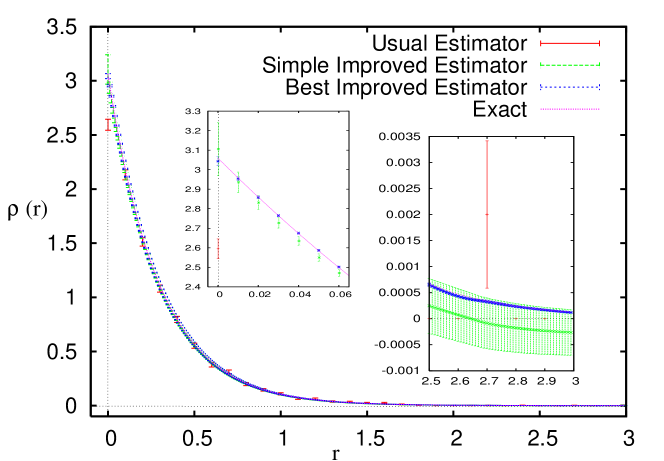
Figure 1:

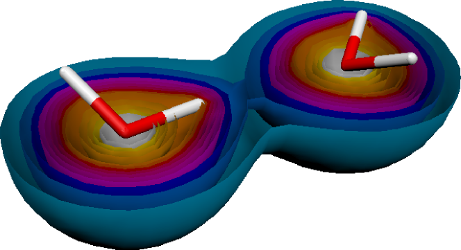
Figure 2:

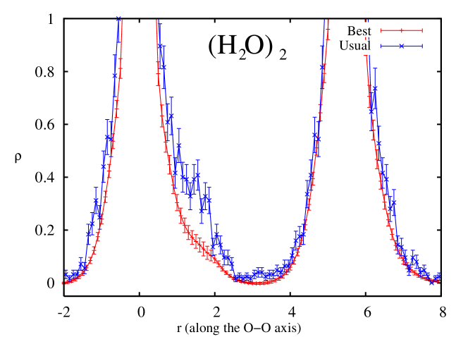
Figure 3:

References

- (1) See, e.g., K. Binder and D. W. Heermann, Monte Carlo Simulation in Statistical Physics : An Introduction (Springer Series in Solid-State Sciences, 80), Springer-Verlag, 1998.
- (2) See, e.g., D.M. Ceperley, Rev. Mod. Phys. 67, 279 (1995).
- (3) N. Metropolis, A. Rosenbluth, M. Rosenbluth, A. Teller, and E. Teller, J. Chem. Phys. 21, 1087 (1953).
- (4) R. Assaraf and M. Caffarel, Phys. Rev. Lett. 83 , 4682 (1999).
- (5) R. Assaraf and M. Caffarel, J. Chem. Phys. 113 ,4028 (2000); R. Assaraf, ibid. 119, 10536 (2003).
- (6) J. Hiller, J. Sucher, G. Feinberg, Phys. Rev. A 18, 2399 (1978).
- (7) J. Sucher and R.J. Drachman, Phys.Rev.A 20, 424 (1979).
- (8) J.E. Harriman, Int. J. Quantum Chem. 17, 689 (1980).
- (9) V.A. Rassolov and D.M. Chipman, J. Chem. Phys. 105, 1470 (1996).
- (10) J. Vrbik, M.F. de Pasquale, S.M. Rothstein, J. Chem. Phys. 88, 3784 (1988).
- (11) P. Langfelder, S.M. Rothstein, J. Vrbik, J. Chem. Phys. 107 8525 (1997).
- (12) S.A. Alexander and R.L. Coldwell, J. Mol. Phys.(Theochem) 487 67 (1999).
- (13) S.R. Gadre, S.A. Kulkarni, and I.H. Shrivastava, J. Chem. Phys. 96 5253 (1992).
- (14) R. F. W. Bader, Atoms in Molecules: A Quantum Theory (Clarendon, Oxford, 1990).
- (15) See, e.g., R. van Leeuwen and E.J. Baerends, Phys. Rev. A 49, 2421 (1994); C.J. Umrigar and X. Gonze, Phys. Rev. A 50, 3827 (1994); Q. Zhao, R. C. Morrison, and R.G. Parr, Phys. Rev. A 50, 2138 (1994); R. C. Morrison and Q. Zhao, Phys. Rev. A 51, 1980 (1995);
- (16) G.S. Tschumper, M.L. Leininger, B.C. Hoffman, E.F. Valeev, H.F. Schaefer III, and M. Quack, J. Chem. Phys. 116 690 (2002).
FIGURE CAPTIONS
-
•