Classifying the expansion kinetics and critical surface dynamics of growing cell populations

Abstract

Based on a cellular automaton model the growth kinetics and the critical surface dynamics of cell monolayers is systematically studied by variation of the cell migration activity, the size of the proliferation zone and the cell cycle time distribution over wide ranges. The model design avoids lattice artifacts and ensures high performance. The monolayer expansion velocity derived from our simulations can be interpreted as a generalization of the velocity relationship for a traveling front in the Fisher-Kolmogorov-Petrovskii-Piskounov (FKPP) equation that is frequently used to model tumor growth phenomena by continuum models. The critical surface dynamics corresponds to the Kardar-Parisi-Zhang (KPZ) universality class for all parameters and model variations studied. While the velocity agrees quantitatively with experimental observations by Bru et al, the critical surface dynamics is in contrast to their interpretation as generic molecular-beam-epitaxy-like growth.

Model simulations of tumor growth and therapy have attracted wide interest GatenbyMaini2003 -DrasdoHoehme2005 . An important issue to which models can contribute is the classification of the tumor growth pattern by generic mechanisms at the level of the individual cell actions (migration, division etc.). These actions subsume the effect of the molecular inter-and intra-cellular regulation. The models can serve to identify those cell activities that would result in a maximal inhibition of multi-cellular growth and invasion, and thereby help to identify possible molecular drug targets. Bru et al BruAlbSubGarcBru2003:BruEtAl03 analyzed the growth kinetics and critical surface dynamics of many different tumors in-vitro and in-vivo. They quantified the dynamics of the tumor surface by three critical exponents used to classify crystal growth phenomena into universality classes BarabasiStanley1995:BaSt95 . They found a generic linear growth phase of in-vitro growing cell lines for large cell populations and a molecular-beam-epitaxy (MBE)-like dynamics of the tumor surface both in-vitro and in-vivo. They proposed a tumor therapy based on these findings BruEtAl2004 .
In this letter we analyze a class of cellular automaton (CA) tumor growth models on an irregular lattice by extensive computer simulations. CA tumor growth models enjoy wide interest MoreiraDeutsch2002 since they permit to represent each cell individually at moderate computational expense. In our model cells can divide, push neighbor cells and migrate. The choice of the model rules is guided by comparison with an off-lattice model. By using the irregular lattice we ensure isotropy and homogeneity of space, and cell sizes that are sharply peaked around a prescribed average value. Both the expansion speed and the spatial pattern formed differ from results on a periodic lattice. We systematically analyze our growth model with respect to the hopping rate, proliferation depth and dispersion of the cell cycle time distribution and show that the expansion dynamics can be mapped onto the functional form of the traveling wave velocity of the Fisher-Kolmogorov-Petrovskii-Piskounov (FKPP) equation Murray1989 . The model reproduces the monolayer expansion kinetics experimentally found by Bru BruAlbSubGarcBru2003:BruEtAl03 . The critical surface growth dynamics suggests a Kadar-Parisi-Zhang (KPZ)-like KPZ1986 behavior over a wide range of parameters and for varying cell migration mechanisms, supporting the critical comment by Buceta and Galeano BucetaGaleano2005 on the conjecture by Bru et. al. BruAlbSubGarcBru2003:BruEtAl03 . Our findings comply with the results in the classical Eden model Moro2001 .

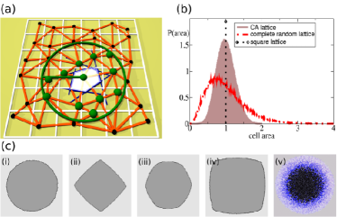
Figure 1: (Color online) (a) Construction of the CA lattice: One point (black, green) is placed in every square of a square lattice at a random position $\underline{r}_{i}$. A Voronoi tesselation is constructed form these points such that each cell consists of all points in space that are closer to the lattice point $\underline{r}_{i}$ than to any other $\underline{r}_{k}$. The shape of a biological cell (white) is identified with the corresponding Voronoi polygon (blue lines). Polygons that share a common edge are defined as neighboring and connected by red lines (Delauney triangulation). (b) Probability density distribution of the cell area for the CA-lattice in (a) (brown) and for a random initial distribution of points (red). (c) Cell cluster morphology for $m=10^{4}$, $\Delta L=1$ on (i) the CA lattice in (a), (ii) square-, (iii) hexagonal lattice, (iv) lattice with Moore neighborhood (nearest neighbors along the axes and the diagonals), (v) off-lattice cluster DrasdoHoehme2005 ; Drasdo2005 .

Our model is based upon the following assumptions:
$[R1]$ Lattice generation: Starting from a regular square lattice with spacing $l$, an irregular lattice $\underline{r}_{i}$ is generated by Delauney triangulation. A biological cell is represented as shown in Fig.1(a) (white).
$[R2]$ Exclusion principle: Each lattice site can be occupied by at most one single cell.
$[R3]$ Cycle time: The cell cycle time $\tau^{\prime}$ is Erlang distributed (with a parameter $m$):

$$f(\tau^{\prime})=\lambda_{m}\frac{(\lambda_{m}\tau^{\prime})^{m-1}}{(m-1)!}exp\{-\lambda_{m}\tau^{\prime}\}$$ (1)

with $\lambda_{m}=m$ such that $\langle\tau^{\prime}\rangle\equiv\tau=1$.
$[R4]$ Proliferation depth: A cell can divide if and only if there is at least one free neighbor site within a circle of radius $\Delta L$ around the dividing cell (Fig. 1 (a), green).
$[R5]$ Cell migration: We consider three alternative migration rules: R5(i) A cell moves with rate $\phi$ to a free neighbor site, irrespectively of the number of neighbor cells before and after its move. This rule corresponds to the case of no cell-cell adhesion. R5(ii) Cells move with rate $\phi$ if by this move the cell is not isolated. R5(iii) Cells move with a rate $\phi\exp\{-\Delta E/F_{T}\}$ with $\Delta E=E(t+\Delta t)-E(t)$, where $\Delta t$ is the time step, $E(t)$ is the total interaction energy of the multi-cellular configuration, $F_{T}\sim 10^{-16}J$ is a ”metabolic” energy BeysensForgacsGlazier2000:BFG00 , $\Delta E/F_{T}\sim{\cal O}(1)-{\cal O}(10)$ DrasdoHoehme2005 . This induces migration towards locations with a larger number of neighbor cells.
By [R1] we generate an unstructured lattice with a symmetric cell area distribution sharply peaked around its average $A=l^{2}$ (see Fig.1 (a),(b)). [R3] considers that experiments indicate a $\Gamma$-like distribution of the cell cycle controlled by cell cycle check points AlbertsEtAl2002 . [R4] takes into regard that the growth speed of tumors is usually incompatible with the assumption that only cells at the border are able to divide (as in the Eden model Eden1961:ME61 , see DrasdoHoehme2005 ). Therefore we assume that a dividing cell is able to trigger the migration of at most $k$ neighbor cells into the direction of minimum mechanical stress (see Fig.1 (a)). If a cell divides, one of its daughter cells is placed at the original position, the other cell is placed next to it and the local cell configuration is shifted and re-arranged along the line that connects the dividing cell with the closed free lattice site within a circle of radius $\Delta L$ such that the latter is now occupied (see Fig.1 (a)). This algorithm mimics a realistic re-arrangement process that may occur from active cell migration as a response to a mechanical stimulus, cf. Ref. KansalEtAl2000 . Isolated cells perform a random-walk-like motion (e.g. Schienbein1994:SchFrGru94 ). We consider different migration rules R5(i)-(iii) to comprise a class of potential models with biologically realistic behavior.
The model parameters are the average cell cycle time $\tau$ and its distribution $f(\tau^{\prime})$ controlled by the parameter $m$, the migration rate $\phi$, the proliferation depth $\Delta L$, and, in case of an energy-activated migration rule, the energy $E$. Programmed cell death can easily be integrated apoptosis but is omitted here. Rules [R1-R5] can be formalized by the master equation

$$\partial_{t}p(Z,t)=\sum_{Z^{\prime}\rightarrow Z}W_{Z^{\prime}\rightarrow Z}p(Z^{\prime},t)-W_{Z\rightarrow Z^{\prime}}p(Z,t).$$ (2)

Here $p(Z,t)$ denotes the multivariate probability to find the cells in configuration $Z$ and $W(Z^{\prime}\rightarrow Z)$ denotes the transition rate from configuration $Z^{\prime}$ to configuration $Z$. A configuration $Z=\{...,x_{i-1},x_{i},x_{i+1},...\}$ consists of local variables $x_{i}=\{0,1\}$ with $x_{i}=0$ if lattice site $i$ is empty, and $x_{i}=1$ if it is occupied by a cell. For the simulation we use the Gillespie algorithm Gillespie1976 , i.e, the time-step of the event-based simulation is a random number given by $\Delta t=-\frac{1}{W_{Z}}ln(1-\xi)$. Here, $\xi$ is a random number equidistributed in $[0,1)$, $W_{Z}=\sum_{Z^{\prime}}W_{Z^{\prime}\rightarrow Z}$ is the sum of all possible events which may occur at time $t$. Here we assume that the rate at which a cell changes its state by a hop, a progress in the cell cycle, or a division is independent of the number of accessible states as long as at least one state, that is, one free adjacent lattice site in case of a hop and one free site within a circle of radius $\Delta L$ in case of a division, is accessible. This may be justified by noting that cells - in contrast to physical particles - are able to sense their environment and therefore the direction into which they can move.
We analyze the growth kinetics by the cell population size $N(t)$ (number of cells at time $t$) and the radius of gyration $R_{gyr}(t)=\sqrt{\frac{1}{N}\sum_{i=1}^{N}(\underline{r}_{i}-\underline{R}_{0})^{2}}$. Here $\underline{R}_{0}=\frac{1}{N}\sum_{i=1}^{N}\underline{r}_{i}$ is the position of the center of mass. For a compact circular cell aggregate (in $d=2$ dimensions), $R_{gyr}$ is related to the mean radius $\overline{R}(t)=\frac{1}{2\pi}\int_{0}^{2\pi}R(\varphi,t)d\varphi$ (polar angle $\varphi$) of the aggregate by $\overline{R}=R_{gyr}\sqrt{2}$.
To interpret the rules and parameters of the CA model in terms of growth mechanisms we compare it with the stochastic single-cell-based off-lattice growth model in Ref. DrasdoHoehme2005 (Fig. 2). In this model cell motion contains an active random component and a component triggered by mechanical forces between cells, and between cells and the substrate ChuEtAl2005 . During cell division the cell gradually deforms and divides into two daughter cells as long as the degree of deformation and compression is not too large.

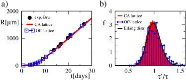
Figure 2: (Color online) (a) Mean radius $\overline{R}$ of the cell aggregate vs. time $t$. Full circles: experimental findings for C6 rat astrocyte glioma cells (BruAlbSubGarcBru2003:BruEtAl03 ). (b) Cell cycle time distribution $f(\tau^{\prime})$ for the off-lattice model and the CA growth model in comparison with the Erlang distribution. ($m=60$, $\Delta L=9$, $\phi=0$)

As illustrated in Fig. 2 the lattice model is able to capture the behavior of the off-lattice model and agrees with the experimental findings in Refs. BruAlbSubGarcBru2003:BruEtAl03 provided the parameters $\Delta L$, $\phi$, $\tau$, $m$ are chosen properly. $\Delta L$ controls the effective thickness of the proliferative rim; in the off-lattice model it depends on the mechanisms that control the proliferation by contact inhibition, on the material properties of the cell (the Young modulus, the Poisson number etc.), and on the ability of a cells to move in response to a mechanical stimulus DrasdoHoehme2005 .
At large $m$ the tumor border becomes smoother and the tumor shape reflects the symmetry of the underlying lattice (Fig. 1 (c)(ii-iv)); this effect is known as noise reduction BatchelorHenry1981 . Such lattice-induced asymmetries could significantly disturb the analysis of the surface growth dynamics in circular geometries. We have chosen a Voronoi tesselation, in which such artifacts do not occur (Fig. 1 (a),(c)(i)). Fig. 3 shows a systematic study of the growth kinetics for free hopping (Rule R5(i)). All quantities are plotted in multiples of $\tau$ and $l$, which are the reference time and length scale, respectively. Initially, the cell population size grows exponentially fast with $N(t)=N(0)exp(t/\tau_{\mathrm{eff}})$ where $\tau_{\mathrm{eff}}^{-1}=(2^{1/m}-1)m\tau^{-1}$ Drasdo2005 . The duration of the initial phase increases with $\Delta L$ and $\phi$. The growth law for the diameter depends on $\phi$. If $\phi=0$, the initial expansion of the diameter is exponentially fast, too. If $\phi>0$, cells initially detach from the main cluster and the diameter grows diffusively, with $L\equiv 2\sqrt{2}R_{gyr}\propto\sqrt{A(\phi+1/\tau_{\mathrm{eff}})t}$ where $A\approx 1.2$ is a lattice-dependent fit constant (Fig. 3(a)). For $t/\tau\leq 2$, $R_{gyr}\propto t$ (Fig. 3(a)). This regime disappears for $N(0)\gg 1$ (see Drasdo2005 ). As soon as cells in the interior of the aggregate are incapable of further division the exponential growth crosses over to a linear expansion phase.

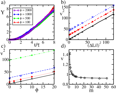
Figure 3: (Color online) (a) $Y=R_{gyr}^{2}/(\phi+1/\tau_{\mathrm{eff}})$ vs. $t/\tau$ for $m=0$, $\Delta L=1$ and different values for $\phi$. (b-d): Growth in the linear expansion regime ($N\sim 10^{5}$). (b) Square of expansion velocity, $v^{2}$, vs. square of the proliferation zone, $\Delta L^{2}$ (triangles: $\phi=0$, circles: $\phi=10$, squares: $\phi=20$; $m=0$). (c) $v^{2}$ vs. $\phi$ (triangles: $\Delta L=1$, circles: $\Delta L=3$, squares: $\Delta L=6$, stars: $\Delta L=10$; $m=0$). (d) $v$ vs. $m$ ($\Delta L=1$, $\phi=0$). The lines are fits using eqn. (3).

Fig. 3 shows $v^{2}$ vs. (b) $(\Delta L)^{2}$, (c) $\phi$, and (d) $m$ for large $N$ ($N\sim 10^{5}$ cells). The model can explain the experimentally observed velocity-range in Ref. BruAlbSubGarcBru2003:BruEtAl03 . As $t\rightarrow\infty$, $L=v(m,\phi,\Delta L)t$ with

$$v^{2}\approx B^{2}([\Delta L^{\prime}(\Delta L)]^{2}/\tau_{\mathrm{eff}}^{2}+\phi/\tau_{\mathrm{eff}}),$$ (3)

$B\approx 1.4$ (lines in Fig. 3b-c). $\Delta L^{\prime}(\Delta L)$ ($\approx 1+0.6(\Delta L-1)$) results from the average over all permutations to pick boundary cells within a layer of thickness $\Delta L$. For $\Delta L/\tau_{\mathrm{eff}}\ll\sqrt{\phi/\tau_{\mathrm{eff}}}$ eqn. (3) has the same form as for the FKPP equation. (e.g. Moro2001 ).

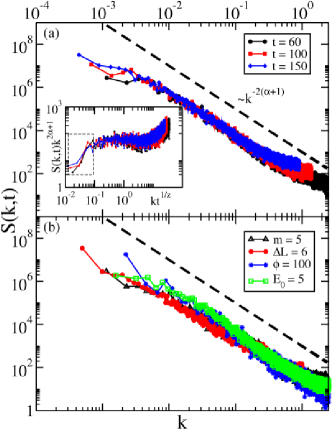
Figure 4: (Color online) (a) Dynamic structure function $S(k,t)$ vs. $k$ for [R5(i)], $\Delta L=0$, $\phi=0$, $m=0$. Inset: rescaled function $S(k,t)k^{2\alpha+1}$ vs. $kt^{1/z}$ ($\alpha=0.5$, $z=3/2$). (b) $S(k,t)$ vs. $k$ for four alternative parameter sets: (A) triangles: $m=5$ ($\Delta L=0$, $\phi=0$), (B) circles: $\Delta L=6$ ($m=0$, $\phi=0$), (C) stars: R5(ii) $\phi=100$ ($m=0$, $\Delta L=0$), (D) squares: R5(iii) $\Delta E/F_{T}=E_{0}+n\cdot E_{B}$ with $E_{B}=10$, $n$ neighbors, $E_{0}=5$ surface binding ($m=0$, $\Delta L=0$) comment_strfnc . The dashed lines are guides to the eye showing $\alpha=0.5$.

Next, to determine the universality class we determine the roughness exponent $\alpha$ and the dynamic exponent $z$ from the dynamic structure function $S(k,t)=\langle R(k,t)R(-k,t)\rangle$ where $R(k,t)$ is the Fourier transform of the local radius $R(s,t)$ and $\langle...\rangle$ denotes the average over different realizations of the growth process (e.g. RamascoLopezRodriguez2000:RaLoRo00 ). Here $s$ is the arclength as in Ref. BruAlbSubGarcBru2003:BruEtAl03 . The third exponent, the growth exponent $\beta$, can be obtained from the scaling relation $\beta=\alpha/z$. In test simulations comparing constant angle segments $\Delta\varphi$ with constant arclength intervals $\Delta s$ we did not find noteworthy differences. For self-affine surfaces in absence of any critical length-scale the dynamic structure function has the Family-Vicsek scaling form FamilyVicsek1985:FaVi85 :

$$S(k,t) = k^{-(2\alpha+1)}s(kt^{1/z})$$ (4)

$$s(u=kt^{1/z}) = \left\{\begin{array}[]{ccc}const.&if&u\gg 1\\ u^{-(2\alpha+1)}&if&u\ll 1.\end{array}\right.$$ (7)

At $u=1$ a crossover occurs. For $u\gg 1$ curves measured at different times collapse onto a single line; at $u\ll 1$ they split. We have calculated $S(k,t)$ for rules R5(i) and $\phi\geq 0$, R5(ii) and R5(iii) (Fig. 4). The final cell population size was of ${\cal O}(10^{5})$ cells which is the typical size of the cell populations in Ref. BruAlbSubGarcBru2003:BruEtAl03 . All these results suggest KPZ-like dynamics with $\alpha=1/2$, $z=3/2$ and $\beta=1/3$ rather than the MBE universality class, i.e., critical exponents $\alpha=3/2$, $z=4$ and $\beta=3/8$ inferred in BruAlbSubGarcBru2003:BruEtAl03 . The parameter range of $\phi\in[0,100)$ captures most cell lines studied in Ref. BruAlbSubGarcBru2003:BruEtAl03 (for $l=10\mu m$, $\tau=24h$, $\phi=100$ corresponds to a diffusion constant of $D=10^{-10}cm^{2}/s$).

In conclusion we have analyzed the expansion kinetics and critical surface dynamics of two-dimensional cell aggregates by extensive computer simulations within a CA model which avoids artifacts from the symmetry of regular lattices. The growth scenarios are compatible with experimental observations. The asymptotic expansion velocity has a form that is reminiscent of the front velocity of the FKPP equation. The same expansion velocity can be obtained for different combinations of the migration and division activities of the cell and of the cycle time distribution. Recently, mathematical models based on the FKPP equation were used to predict the distribution of tumor cells for high-grade glioma in regions which are below the detection threshold of medical image techniques SwansonAlvordMurray2000:SwAlMu00 . We believe such predictions must fail since the FKPP equation lacks some important parameters such as the proliferation depth which is why it is not sensitive to relative contributions of the proliferation depth and free migration. We observed in our simulations that these relative contributions in fact determine the cell density profile at the tumor-medium interface: the larger the fraction of free migration is, the wider is the front profile even if the average expansion velocity is constant.
The critical surface dynamics found in our simulations does not comply with the interpretation of experimental observations by Bru et. al. BruAlbSubGarcBru2003:BruEtAl03 even for the migration mechanism they suggested (R5(iii)). We propose to re-analyze the corresponding experiments and track the paths of marked cells.

Support within Sfb 296 (MB) and by DFG grant BIZ 6-1/1 (DD) is acknowledged.

References

- (1) R. A. Gatenby and P. K. Maini, Nature 421, 321 (2003).; D.-S. Lee, H. Rieger, and K. Bartha, Phys. Rev. Lett. 96, 058104 (2006).
- (2) J. Krug and H. Spohn, in Solids Far From Equilibrium: Growth, Morphology and Defects, edited by C. Godreche (Cambridge University Press, Cambridge, 1991).; J. Moreira and A. Deutsch, Adv. Compl. Syst. 5, 247 (2002).
- (3) D. Drasdo and S. Hoehme, Phys. Biol. 2, 133 (2005).
- (4) A. Brú, J. M. Pastor, I. Fernaud, I. Brú, S. Melle, and C. Berenguer, Phys. Rev. Lett. 81, 4008 (1998).; A. Brú, S. Albertos, J. L. Subiza, J. L. García-Asenjo, and I. Brú, Biophys. J. 85, 2948 (2003).
- (5) A.-L. Barabási and H. E. Stanley, Fractal concepts in surface growth (Cambridge University Press, 1995).
- (6) A. Brú, S. Albertos, J. L. García-Asenjo, and I. Brú, Phys. Rev. Lett. 92, 238101 (2004).; and J. Clin. Invest. 8, 9 (2005).
- (7) J. Murray, Mathematical Biology (Oxford University Press, Oxford, U.K., 1989).
- (8) M. Kardar, G. Parisi, and Y.-C. Zhang, Phys. Rev. Lett. 56, 889 (1986).
- (9) J. Buceta and J. Galeano, Biophys. J. 88, 3734 (2005).
- (10) E. Moro, Phys. Rev. Lett. 87, 238303 (2001).
- (11) D. Beysens, G. Forgacs, and J. Glazier, Proc. Natl. Acad. Sci. USA 97, 9467 (2000).
- (12) B. Alberts, A. Johnson, J. Lewis, M. Raff, K. Roberts, and P. Walter, The Cell, 3rd ed. (Garland Science Publ., New York, 2002).
- (13) M. Eden, in Proc. of the 4th. Berkeley Symposium on Mathematics and Probability, edited by J. Neyman (Univ. of California Press, Berkeley, 1961), pp. 223 – 239.
- (14) A. R. Kansal, S. Torquato, G. R. I. Harsh, E. A. Chiocca, and T. S. Deisboeck, J. Theor. Biol. 203, 367 (2000).
- (15) M. Schienbein, K. Franke, and H. Gruler, Phys. Rev. E 49, 5462 (1994).
- (16) D. T. Gillespie, J. Comput. Phys. 22, 403 (1976); this algorithm is also known as Bortz-Kalos-Lebowitz algorithm: A. B. Bortz, M. H. Kalos, and J. L. Lebowitz, J. Comp. Phys. 17, 10 (1975).
- (17) Y.-S. Chu, S. Dufour, J. P. Thiery, E. Perez, and F. Pincet, Phys. Rev. Lett. 94, 028102 (2005).
- (18) D. Drasdo, Adv. Compl. Syst. 2 & 3, 319 (2005).
- (19) M. Batchelor and B. Henry, Phys. Lett. A 157, 229 (1991).
- (20) We have also tested vs. for R5(i), , , and found .
- (21) We mainly found a rescaling of the proliferation rate to ( is the rate of programmed cell death).
- (22) J. Ramasco, J. Lopez, and M. Rodriguez, Phys. Rev. Lett. 84, 2199 (2000).
- (23) F. Family and T. Vicsek, J. Phys. A 18, L75 (1985).
- (24) K. R. Swanson, E. C. Alvord, and J. D. Murray, Cell Prolif. 33, 317 (2000); E. Mandonnet, J.-Y. Delattre, M. L. Tanguy, K. R. Swanson, A. F. Carpentier, H. Duffau, P. Cornu, R. van Effenterre, E. C. Jr Alvord, and L. Capelle, Ann. Neurol. 53, 524 (2003).