Theory of x-ray absorption by laser-dressed atoms

Abstract

An ab initio theory is devised for the x-ray photoabsorption cross section of atoms in the field of a moderately intense optical laser ($800\,{\rm{nm}}$, $10^{13}\,{\rm{{{W}\over{cm^{2}}}}}$). The laser dresses the core-excited atomic states, which introduces a dependence of the cross section on the angle between the polarization vectors of the two linearly polarized radiation sources. We use the Hartree-Fock-Slater approximation to describe the atomic many-particle problem in conjunction with a nonrelativistic quantum-electrodynamic approach to treat the photon–electron interaction. The continuum wave functions of ejected electrons are treated with a complex absorbing potential that is derived from smooth exterior complex scaling. The solution to the two-color (x-ray plus laser) problem is discussed in terms of a direct diagonalization of the complex symmetric matrix representation of the Hamiltonian. Alternative treatments with time-independent and time-dependent non-Hermitian perturbation theories are presented that exploit the weak interaction strength between x rays and atoms. We apply the theory to study the photoabsorption cross section of krypton atoms near the $K$ edge. A pronounced modification of the cross section is found in the presence of the optical laser.

I Introduction

The ionization of an atom by a strong optical field may, under suitable conditions, be described by a tunneling model Delone and Krainov (2000). The Ammosov-Delone-Krainov tunneling formula Ammosov et al. (1986) predicts that ionization out of a sublevel with an orbital angular momentum projection quantum number $m=0$ is strongly preferred over ionization from $m=\pm 1$ sublevels. Employing a relatively intense laser, $I=10^{14}$–$10^{15}\,{\rm{{{W}\over{cm^{2}}}}}$, Young et al. Young et al. (2006) studied laser-induced ionization of krypton atoms from the $4p$ sublevel. By monitoring the $1s\to 4p$ resonance with a subsequent x-ray pulse at a photon energy of $14.3\,{\rm{keV}}$, they were able to measure a background-free signature of the laser-produced $4p$ vacancy for several angles between laser and x-ray polarizations. The data exhibited a clear fingerprint of orbital alignment; yet the x-ray absorption ratio between parallel and perpendicular polarizations was significantly lower than that predicted by the nonrelativistic tunneling picture Ammosov et al. (1986). By including the impact of spin-orbit coupling in the valence shell of krypton, the experimental findings could be explained Santra et al. (2006).

In the experiment of Young et al. Young et al. (2006), the laser was strong enough to ionize the krypton atoms, so that x-ray absorption probed krypton ions. A related scheme is the following. If one overlaps the laser and x-ray fields in both space and time, but keeps the laser intensity just low enough to avoid excitation of the closed-shell atoms in their ground state, then the effect of the laser field is to modify the final states that a core electron can reach via x-ray absorption. This scenario—x-ray absorption by laser-dressed noble-gas atoms (see also Ref. Buth et al., 2007)—is the subject of an ongoing experiment at Argonne National Laboratory and motivated our theoretical studies.

Certain aspects of the theory of x-ray absorption by laser-dressed atoms were analyzed in Refs. Freund, 1973; Ehlotzky, 1975; Jain and Tzoar, 1977; Ehlotzky, 1978; Ferrante et al., 1981a, b; Kálmán, 1988; Fonseca and Nunes, 1988; Kálmán, 1989a, b; Cionga et al., 1993; Glover et al., 1996. Freund Freund (1973) treats the simultaneous absorption of one laser photon and one x-ray photon by solids. The absorption of x rays by laser-dressed hydrogen is examined in Refs. Leone et al., 1988; Kálmán, 1989b; Cionga et al., 1993. Particularly, Cionga et al. Cionga et al. (1993) and Kálmán Kálmán (1989b) point out the importance of laser-dressing effects close to the ionization threshold. Leone et al. Leone et al. (1988) and Ferrante et al. Ferrante et al. (1981a) study the angular distribution of the photoelectrons. References Freund, 1973; Ehlotzky, 1975; Jain and Tzoar, 1977; Ehlotzky, 1978; Ferrante et al., 1981a, b; Kálmán, 1988; Fonseca and Nunes, 1988; Kálmán, 1989a, b; Cionga et al., 1993; Glover et al., 1996 have in common that they treat the final state of the excited electron following x-ray absorption essentially as a Volkov-type wave. Some of them include a Coulomb correction. They do not describe the element-specific properties of the x-ray absorption cross section in the immediate vicinity of an inner-shell edge.

The energy spectrum of photoelectrons generated through XUV photoionization of helium in the presence of an intense laser field was measured in Refs. Glover et al., 1996; Guyétand et al., 2005. The laser-induced modification of the x-ray absorption near-edge structure (XANES) Rehr and Albers (2000); Als-Nielsen and McMorrow (2001) has not yet been experimentally investigated for any laser-dressed atom or molecule. In molecules, it must be expected that an external laser field will also have an impact on the extended x-ray absorption fine structure (EXAFS) Rehr and Albers (2000); Als-Nielsen and McMorrow (2001). Therefore, in addition to its fundamental interest, understanding the laser-dressing effect on x-ray absorption is important from a practical point of view. For instance, if one adiabatically aligns a molecule using an intense laser pulse Stapelfeldt and Seideman (2003) and performs a XANES or EXAFS measurement in order to determine molecular structure information, then one has to be able to correct for the artificial impact of the aligning laser pulse on the x-ray absorption cross section.

In this paper, we devise an ab initio theory for the x-ray absorption cross section of an isolated atom in the presence of an optical laser. The Hartree-Fock-Slater mean-field model Slater (1951); Slater and Johnson (1972) is utilized to treat the atomic many-electron problem. This choice is adequate as shakeup and shakeoff effects are generally weak in inner-shell photoionization. They do not play a role in the immediate vicinity of the respective inner-shell edge. To describe the radiation fields, we use a quantum-electrodynamic framework which is equivalent to the semiclassical Floquet theory in the limit of high laser intensities. The coupling of the x rays to the atom is described perturbatively. The laser dressing of the final-state manifold, however, is treated nonperturbatively. The theory is implemented in terms of the program dreyd as part of the fella package Buth and Santra (2006). We apply our method to study the x-ray absorption cross section of laser-dressed krypton atoms near the $K$ edge. Its dependence on the x-ray photon energy and on the angle between the polarization vectors of the laser and the x rays is investigated.

The article is structured as follows. Section II discusses the theoretical foundation of the two-color problem of an x-ray probe of a laser-dressed atom using an independent-particle model for the atomic electrons, quantum electrodynamics for the photons, and a complex absorbing potential for the continuum electron. The conservation of the energy-integrated x-ray absorption cross section is also investigated. Subsequently, the theory is applied to a krypton atom; computational details are given in Sec. III; the results are presented in Sec. IV. Conclusions are drawn in Sec. V.

Our equations are formulated in atomic units. The Bohr radius $1\,{\rm{bohr}}=1\,a_{0}$ is the unit of length and $1\,t_{0}$ represents the unit of time. The unit of energy is $1\,{\rm{hartree}}=1\,{\rm{\mathit{E}_{\mathit{h}}}}$. Intensities are given in units of $1\,{\rm{\mathit{E}_{\mathit{h}}}}\>t_{0}^{-1}\,a_{0}^{-2}=6.43641\times 10^{15}\,{\rm{W\,cm^{-2}}}$.

II Theory

II.1 Quantum electrodynamic treatment of atoms

We solve the atomic many-electron problem in terms of a nonrelativistic one-electron model. Within this framework, each electron moves in the field of the atomic nucleus and in a mean field generated by the other electrons. The best such mean field derives from the Hartree-Fock method Szabo and Ostlund (1989). However, the Hartree-Fock mean field is nonlocal, due to the exchange interaction, and therefore cumbersome to work with. Slater Slater (1951) introduced a local approximation to electron exchange, which is the principle underlying the well-known $X\alpha$ method Slater and Johnson (1972). The resulting one-electron potential, $V_{\mathrm{HFS}}(r)$, is a central potential, which satisfies

$$V_{\mathrm{HFS}}(r)\rightarrow-{{Z}\over{r}}&\quad\hbox{for}\quad r\rightarrow 0\;,\\ V_{\mathrm{HFS}}(r)\rightarrow-{{1}\over{r}}\quad\hbox{for}\quad r\rightarrow\infty$$ (1)

for a neutral atom of nuclear charge $Z$. In this approximation, the atomic Hamiltonian is given by

$$\hat{H}_{\mathrm{AT}}=-{{1}\over{2}}\vec{\nabla}^{2}+V_{\mathrm{HFS}}(r)\;.$$ (2)

In spherical polar coordinates, its eigenfunctions, the so-called atomic orbitals, are the one-electron wave functions of the form Merzbacher (1998)

$$\psi_{n,l,m}(r,\vartheta,\varphi)={{u_{n,l}(r)}\over{r}}\>Y_{l,m}(\vartheta,\varphi)\;.$$ (3)

Here, $n$, $l$, and $m$ are the principal, orbital angular momentum, and projection quantum number, respectively. Using the ansatz (3) with the Hamiltonian (2), we obtain the radial Schrödinger equation

$$\Bigl{[}-{{1}\over{2}}{{\>\mathrm{d}^{2}}\over{\>\mathrm{d}r^{2}}}+{{l(l+1)}\over{2r^{2}}}+V_{\mathrm{HFS}}(r)\Bigr{]}\,u_{n,l}(r)=E_{n,l}\>u_{n,l}(r)\;,$$ (4)

where $E_{n,l}$ is the eigenenergy. Equation (4) is solved in a finite-element basis set Bathe (1976); Bathe and Wilson (1976); Braun et al. (1993); Ackermann and Shertzer (1996); Rescigno et al. (1997); Meyer et al. (1997); Santra et al. (2004)—which is described in detail in Ref. Santra et al., 2004—for $l=0,\ldots,n_{l}-1$; the positive integer $n_{l}$ denotes the number of angular momenta included in the basis set. The calculated eigenfunctions satisfy the boundary conditions $u_{n,l}(r_{\mathrm{min}})=0$ and $u_{n,l}(r_{\mathrm{max}})=0$, where $r_{\mathrm{min}}=0$ and $r_{\mathrm{max}}$ is the maximum extension of the radial grid.

Within the framework of quantum electrodynamics Craig and Thirunamachandran (1984), the Hamiltonian describing the effective one-electron atom interacting with the electromagnetic field reads

$$\hat{H}_{\mathrm{QED}}=\hat{H}_{\mathrm{AT}}+\hat{H}_{\mathrm{EM}}+\hat{H}_{\mathrm{I}}\;.$$ (5)

Here,

$$\hat{H}_{\mathrm{EM}}=\sum_{\vec{k},\lambda}\omega^{\vphantom{{\dagger}}}_{\vec{k}}\,\hat{a}^{{\dagger}}_{\vec{k},\lambda}\hat{a}^{\vphantom{{\dagger}}}_{\vec{k},\lambda}$$ (6)

represents the free electromagnetic field; its vacuum energy has been set to zero. The operator $\hat{a}^{{\dagger}}_{\vec{k},\lambda}$ ($\hat{a}^{\vphantom{{\dagger}}}_{\vec{k},\lambda}$) creates (annihilates) a photon with wave vector $\vec{k}$, polarization $\lambda$, and energy $\omega_{\vec{k}}=c\,|\vec{k}|=|\vec{k}|/\alpha$ with the speed of light $c$ and the fine-structure constant $\alpha$. The light-electron interaction term in electric-dipole approximation is given in the length gauge by Craig and Thirunamachandran (1984)

$$\hat{H}_{\mathrm{I}}=\vec{x}\cdot\sum_{\vec{k},\lambda}{\rm i}\,\sqrt{{{2\pi}\over{V}}\,\omega^{\vphantom{{\dagger}}}_{\vec{k}}}\>\bigl{[}\vec{e}^{\vphantom{\ast}}_{\vec{k},\lambda}\hat{a}^{\vphantom{{\dagger}}}_{\vec{k},\lambda}-\vec{e}^{\>\ast}_{\vec{k},\lambda}\hat{a}^{{\dagger}}_{\vec{k},\lambda}\bigr{]}\;.$$ (7)

We use the symbol $\vec{x}=(x,y,z){}^{\textrm{\scriptsize T}}$ for the atomic dipole operator in Cartesian coordinates. In Eq. (7), $V$ denotes the normalization volume of the electromagnetic field and $\vec{e}_{\vec{k},\lambda}$ indicates the polarization vector of mode $\vec{k},\lambda$. Note that the electrons are treated in first quantization, whereas the electromagnetic field is treated in second quantization.

The eigenstates of $\hat{H}_{\mathrm{AT}}+\hat{H}_{\mathrm{EM}}$ may be written as a direct product of the form $\left|\right.\!\psi_{n,l,m}\!\left.\right>\,\left|\right.\!\{N_{\vec{k},\lambda}\}\!\left.\right>$, where $\left|\right.\!\{N_{\vec{k},\lambda}\}\!\left.\right>$ is the Fock state (or number state) of the photon field with $N_{\vec{k},\lambda}$ photons in the mode $\vec{k},\lambda$. The curly braces indicate that more than one mode may be occupied. The eigenfunctions of $\hat{H}_{\mathrm{QED}}$ cannot, in general, be written in the form $\left|\right.\!\psi_{n,l,m}\!\left.\right>\,\left|\right.\!\{N_{\vec{k},\lambda}\}\!\left.\right>$. They may, however, be expanded in the basis $\{\left|\right.\!\psi_{n,l,m}\!\left.\right>\,\left|\right.\!\{N_{\vec{k},\lambda}\}\!\left.\right>\}$, which we employ in the following.

II.2 Complex absorbing potential

The absorption of photons may lead to the ejection of one or more electrons from an atom; either directly by photoionization or indirectly by the formation and decay of electronic resonances. The ejected electrons are in the continuum and thus their wave functions are not square integrable Kukulin et al. (1989); Moiseyev (1998a); Santra and Cederbaum (2002). Therefore, they cannot be described by the basis set expansion techniques in Hilbert space that are frequently employed in bound-state quantum mechanics Merzbacher (1998); Szabo and Ostlund (1989). Several theories have been developed to make, particularly, resonance states, nevertheless, amenable to a treatment with methods for bound states. They typically lead to a non-Hermitian, complex-symmetric representation of the Hamiltonian Kukulin et al. (1989); Moiseyev (1998a); Santra and Cederbaum (2002). In this framework, resonances are characterized by a complex energy

$$E_{\mathrm{res}}=E_{\mathrm{R}}-{\rm i}\,\Gamma/2\;,$$ (8)

which is frequently called Siegert energy Kukulin et al. (1989); Siegert (1939). Here, $\Gamma$ stands for the transition rate from the specific resonance state to the continuum in which it is embedded.

Noteworthy for this work are complex scaling Reinhardt (1982); Kukulin et al. (1989); Moiseyev (1998a) and complex absorbing potentials (CAP) Goldberg and Shore (1978); Jolicard and Austin (1985, 1986); Neuhauser and Baer (1989); Riss and Meyer (1993, 1995); Moiseyev (1998b); Riss and Meyer (1998); Palao et al. (1998); Palao and Muga (1998); Karlsson (1998); Sommerfeld et al. (1998); Santra and Cederbaum (2001, 2002); Manolopoulos (2002); Poirier and Carrington, Jr. (2003a, b) which are exact methods to determine the resonance energies (8) of a given Hamiltonian. The CAPs have been analyzed thoroughly by Riss and Meyer Riss and Meyer (1993) using complex scaling. Conversely, complex scaling of the Hamiltonian has been used to construct a CAP that is adapted to a specific Hamiltonian Moiseyev (1998b); Riss and Meyer (1998); Karlsson (1998). In all these methods, the resonance wave function associated with $E_{\mathrm{res}}$, Eq. (8), is square-integrable. To devise a CAP for $\hat{H}_{\mathrm{QED}}$ in the spirit of Refs. Moiseyev, 1998b; Riss and Meyer, 1998; Karlsson, 1998, we apply complex scaling to it. This is simply a complex coordinate transformation of the Hamiltonian. Here, only the specialization to the scaling of the radial coordinate $r=|\vec{x}|$ is needed, which proceeds in complete analogy to the one-dimensional case of Refs. Moiseyev, 1998b; Karlsson, 1998.

The radial part $r$ of the electron coordinates is replaced by a path in the complex plane $\varrho\equiv F(r)$ Reinhardt (1982); Moiseyev (1998a); the resulting position vector is $\vec{\chi}=\varrho\>(\cos\varphi\,\sin\vartheta,\,\sin\varphi\,\sin\vartheta,\,\cos\vartheta){}^{\textrm{\scriptsize T}}$ with the polar angle $\vartheta$ and the azimuth angle $\varphi$ Arfken (1970). We use the path of Moiseyev Moiseyev (1998b) in the form of Karlsson Karlsson (1998)

$$F(r)=r+(\mathrm{e}^{{\rm i}\theta}-1)\Bigl{[}r+r_{0}+{{1}\over{2\lambda}}\ln\Bigl{(}{{1+\mathrm{e}^{2\lambda(r-r_{0})}}\over{1+\mathrm{e}^{2\lambda(r+r_{0})}}}\Bigr{)}\Bigr{]}\;.$$ (9)

Please refer to Refs. Moiseyev, 1998b; Karlsson, 1998 for a graphical representation. The path starts at $r=0$ and runs along the positive real axis, i.e., $F(r)\approx r$. In the vicinity of some distance $r_{0}$ from the origin, the so-called exteriority, it bends into the upper complex plane. The bending is smooth, i.e., $F(r)$ is infinitely many times continuously differentiable. For $r\gg r_{0}$, the path becomes the exterior scaling path, i.e., $F(r)\approx r_{0}+(r-r_{0})\,\mathrm{e}^{{\rm i}\theta}$. The parameter $\lambda$ in Eq. (9) is a measure of how smooth the bending around $r_{0}$ is; it is referred to as smoothness of the path. A complex electron coordinate transformation of the Hamiltonian with a smooth path is termed smooth exterior complex scaling (SES) Moiseyev (1998b). Practical computational aspects of SES are discussed in Sec. III.

Let us concentrate on the atomic contribution $\hat{H}_{\mathrm{AT}}$ first. The complex scaled radial Schrödinger equation is obtained by replacing $r$ with $\varrho$ in Eq. (4). It can be simplified following Karlsson Karlsson (1998) (please note that there are various misprints in the equations of Ref. Karlsson, 1998): Letting $f(r)=F^{\prime}(r)$ with ${}^{\prime}={{\>\mathrm{d}}\over{\>\mathrm{d}r}}$, we make the ansatz

$$u_{n,l}(\varrho)=\sqrt{f(r)}\;{{\mu_{n,l}(r)}\over{f(r)}}\;.$$ (10)

Applying the chain rule to rewrite the complex scaled Eq. (4) with the substitution (10), we can extract expressions involving the unscaled operator on the left-hand side of Eq. (4) augmented by a CAP Karlsson (1998). The CAP subsumes all corrective terms that arise from the complex scaled kinetic energy. A further contribution results from the atomic potential. If the exteriority $r_{0}$ is chosen sufficiently large, only the long-range behavior of the atomic potential [cf. Eq. (1)] is affected by complex scaling. Its contribution is added following Ref. Klaiman et al., 2004. Finally, the CAP is given by

$$\hat{W}&=\hat{W}_{\rm k}+\Bigl{(}{{1}\over{2\varrho^{2}}}-{{1}\over{2r^{2}}}\Bigr{)}\,l\,(l+1)-{{1}\over{\varrho}}+{{1}\over{r}}\;,\\ \hat{W}_{\rm k}=-{{1}\over{2}}{{1}\over{f(r)}}{{\>\mathrm{d}^{2}}\over{\>\mathrm{d}r^{2}}}{{1}\over{f(r)}}\\ {}-{{1}\over{8}}{{2f^{\prime\prime}(r)f(r)-3[f^{\prime}(r)]^{2}}\over{f^{4}(r)}}-\Bigl{(}-{{1}\over{2}}{{\>\mathrm{d}^{2}}\over{\>\mathrm{d}r^{2}}}\Bigr{)}\;.$$ (11)

In the interior, $r\ll r_{0}$, we have $f(r)\approx 1$ and thus the scaled kinetic energy becomes the unscaled one such that the correction term $\hat{W}_{\rm k}$ vanishes. Similarly, all other contributions to $\hat{W}$ become negligible and $\hat{W}$ itself vanishes. We will assume throughout that $r_{0}$ is large enough so that the occupied atomic orbitals are unaffected by the CAP.

The complex coordinate transformation of the radial Schrödinger equation (4) modifies the volume element in integrations involving the $u_{n,l}(\varrho)$; it becomes $f(r)\>\mathrm{d}r$. However, using the $\mu_{n,l}(r)$ instead, the integration measure becomes $\>\mathrm{d}r$. Regarding the full Hamiltonian, $\hat{H}_{\mathrm{QED}}$, we note that the free photon field, $\hat{H}_{\mathrm{EM}}$, does not depend on the electronic coordinates and thus makes no contribution to $\hat{W}$. However, the interaction part, $\hat{H}_{\mathrm{I}}$, has to be complex scaled. To keep the notation transparent, we refrain from formulating this transformation in terms of a contribution to $\hat{W}$ but apply complex scaling directly.

The CAP in Eq. (11) is referred to as smooth exterior complex scaling CAP (SES-CAP). It combines the advantages of simple polynomial CAPs Riss and Meyer (1993) on the one hand and complex scaling on the other hand, eliminating many of their disadvantages. First, no optimization with respect to a parameter is required for SES-CAPs to determine resonance energies. Second, the construction of a well-adapted CAP to a specific Hamiltonian is rather straightforward. Third, the resulting SES-CAP expressions are relatively simple and can be evaluated efficiently on computers.

II.3 X-ray probe of a laser-dressed atom

In the following, only two modes (or two colors) of the radiation field are considered: The laser beam with photon energy $\omega_{\mathrm{L}}$ and the x-ray beam with photon energy $\omega_{\mathrm{X}}$. They are assumed to be monochromatic, linearly polarized, and copropagating. The polarization vector $\vec{e}_{\mathrm{L}}$ of the laser defines the quantization axis, which is chosen to coincide with the $z$ axis of the coordinate system. Further, $\vec{e}_{\mathrm{X}}$ denotes the polarization vector of the x-ray beam and $\vartheta_{\mathrm{LX}}$ is the angle between $\vec{e}_{\mathrm{L}}$ and $\vec{e}_{\mathrm{X}}$, i.e., $\vec{e}_{\mathrm{L}}\cdot\vec{e}_{\mathrm{X}}=\cos{\vartheta_{\mathrm{LX}}}$. Let the photon numbers in the absence of interaction with the atom be $N_{\mathrm{L}}$ for the laser mode and $N_{\mathrm{X}}$ for the x-ray mode, respectively. The laser intensity is then given by

$$I_{\mathrm{L}}={{N_{\mathrm{L}}}\over{V}}{{\omega_{\mathrm{L}}}\over{\alpha}}\;,$$ (12)

with the fine structure constant $\alpha={{1}\over{c}}$. Similarly,

$$J_{\mathrm{X}}={{N_{\mathrm{X}}}\over{V}}{{1}\over{\alpha}}$$ (13)

represents the x-ray photon flux.

As other modes do not contribute—radiative corrections are neglected—$\hat{H}_{\mathrm{EM}}$ [Eq. (6)] and the complex scaled $\hat{H}_{\mathrm{I}}$ [Eq. (7)] can be cast in a simplified form,

$$\hat{H}_{\mathrm{EM}} = \omega^{\vphantom{{\dagger}}}_{\mathrm{L}}\,\hat{a}^{{\dagger}}_{\mathrm{L}}\hat{a}^{\vphantom{{\dagger}}}_{\mathrm{L}}+\omega^{\vphantom{{\dagger}}}_{\mathrm{X}}\,\hat{a}^{{\dagger}}_{\mathrm{X}}\hat{a}^{\vphantom{{\dagger}}}_{\mathrm{X}}\;,$$ (14)

$$\hat{H}_{\mathrm{I}} = \vec{\chi}{}^{\textrm{\scriptsize T}}\,{\rm i}\,\sqrt{{{2\pi}\over{V}}\,\omega^{\vphantom{{\dagger}}}_{\mathrm{L}}}\,\bigl{[}\vec{e}^{\vphantom{\ast}}_{\mathrm{L}}\hat{a}^{\vphantom{{\dagger}}}_{\mathrm{L}}-\vec{e}^{\>\ast}_{\mathrm{L}}\hat{a}^{{\dagger}}_{\mathrm{L}}\bigr{]}$$ (15)

$${}+\vec{\chi}{}^{\textrm{\scriptsize T}}\,{\rm i}\,\sqrt{{{2\pi}\over{V}}\,\omega^{\vphantom{{\dagger}}}_{\mathrm{X}}}\,\bigl{[}\vec{e}^{\vphantom{\ast}}_{\mathrm{X}}\hat{a}^{\vphantom{{\dagger}}}_{\mathrm{X}}-\vec{e}^{\>\ast}_{\mathrm{X}}\hat{a}^{{\dagger}}_{\mathrm{X}}\bigr{]}$$

$${}=\hat{H}_{\mathrm{I,L}}+\hat{H}_{\mathrm{I,X}}\;.$$

Note that we rewrite the complex Hermitian scalar product in Eq. (7) in terms of a complex bilinear product here due to the complex scaling Kukulin et al. (1989); Moiseyev (1998a); Santra and Cederbaum (2002). In comparison to all other interactions, the influence of the x-ray field may be considered as weak. We, therefore, separate the total complex scaled Hamiltonian $\hat{H}_{\mathrm{QED}}$ [Eq. (5)] into a strongly interacting part,

$$\hat{H}_{0}=\hat{H}_{\mathrm{AT}}+\hat{H}_{\mathrm{EM}}+\hat{H}_{\mathrm{I,L}}+\hat{W}$$ (16)

and a weakly interacting part

$$\hat{H}_{1}=\hat{H}_{\mathrm{I,X}}\;.$$ (17)

The SES-CAP (11) contains the corrective terms that arise in the complex scaling of $\hat{H}_{\mathrm{AT}}$. Note that $\hat{H}_{0}$ conserves the atomic angular momentum projection quantum number $m$ and the number of x-ray photons $N_{\mathrm{X}}$. This partition of the Hamiltonian will prove useful below when perturbation theory is applied to the problem.

We are concerned here with the case that $\omega_{\mathrm{X}}$ is large enough to drive the excitation of an electron in the $K$ shell. The x-ray intensity is assumed to be low enough to allow the description of the interaction with the atom in terms of a one-photon absorption process. This assumption is fully valid for experiments at third-generation synchrotron radiation facilities, but may have to be modified for experiments with future free-electron lasers. At such high photon energies, electrons in higher-lying shells are rather insensitive to the x-ray field. On the other hand, inner-shell electrons are unaffected by the laser. As long as the laser intensity is small in comparison to an atomic unit, even the valence shell is only weakly modified, and this modification is expected to be similar before and after the absorption of an x-ray photon by a $K$-shell electron.

Hence, due to the weak coupling to the laser and the x rays, we use a direct product with the unperturbed $1s$ atomic orbital; the initial state of the system before x-ray absorption reads

$$\left|\right.\!I\!\left.\right>=\left|\right.\!\psi_{1,0,0}\!\left.\right>\left|\right.\!N_{\mathrm{L}}\!\left.\right>\left|\right.\!N_{\mathrm{X}}\!\left.\right>\;.$$ (18)

It is an eigenvector of $\hat{H}_{\mathrm{AT}}+\hat{H}_{\mathrm{EM}}$ with eigenvalue

$$E_{I}=E_{1s}+N_{\mathrm{L}}\,\omega_{\mathrm{L}}+N_{\mathrm{X}}\,\omega_{\mathrm{X}}\;.$$ (19)

It is also an approximate eigenvector of $\hat{H}_{0}$ because the SES-CAP may be chosen such that essentially it has no effect on $\left|\right.\!I\!\left.\right>$, i.e., $\left<\right.\!\psi_{1,0,0}\!\left.\right|\hat{W}\left|\right.\!\psi_{1,0,0}\!\left.\right>\approx 0$ holds [see Sec. II.2]. In Eq. (19), $E_{1s}$ is the negative of the binding energy of a $K$-shell electron. In principle, $E_{1s}$ is given by the energy of the atomic $1s$ orbital $E_{1,0}$. Yet $E_{1,0}$ turns out to be not sufficiently accurate [see the caption of Tab. 1]. To place the $K$ edge precisely, we replace $E_{1,0}$ with the experimentally determined $E_{1s}$.

In order to determine the manifold of laser-dressed final states, one needs to observe that $N_{\mathrm{X}}$ is reduced by one unit after x-ray photon absorption and the final states are assumed to be unperturbed by the x rays. Since $\hat{H}_{1}$ couples only the electronic and x-ray degrees of freedom, the accessible final states must have nonzero components with respect to $\left|\right.\!\psi_{n,l,m}\!\left.\right>\left|\right.\!N_{\mathrm{L}}\!\left.\right>\left|\right.\!N_{\mathrm{X}}-1\!\left.\right>$, where $l=1$. The projection quantum number $m$ does not have to be zero, for $\vec{e}_{\mathrm{X}}$ does not necessarily coincide with $\vec{e}_{\mathrm{L}}$, i.e., the angle $\vartheta_{\mathrm{LX}}$ does not have to be zero. We employ the basis formed by the

$$\left|\right.\!\Phi_{n,l,m,\mu}\!\left.\right>=\left|\right.\!\psi_{n,l,m}\!\left.\right>\left|\right.\!N_{\mathrm{L}}-\mu\!\left.\right>\left|\right.\!N_{\mathrm{X}}-1\!\left.\right>\;,$$ (20)

where the quantum numbers $n$, $l$, and $m$ correspond to orbitals that are unoccupied in the atomic ground state. The number of laser photons that are absorbed (emitted) by the core-excited electron is denoted by $\mu=0,\pm 1,\pm 2,\ldots\;$. The operator $\hat{H}_{\mathrm{AT}}+\hat{H}_{\mathrm{EM}}$ is diagonal in this basis with eigenvalues $E_{n,l,\mu}=E_{n,l}+(N_{\mathrm{L}}-\mu)\,\omega_{\mathrm{L}}+(N_{\mathrm{X}}-1)\,\omega_{\mathrm{X}}$; the operator $\hat{H}_{0}$, however, is not. A global energy shift

$$\hat{H}_{\mathrm{EM}}^{\prime}=\hat{H}_{\mathrm{EM}}-N_{\mathrm{L}}\omega_{\mathrm{L}}-[N_{\mathrm{X}}-1]\omega_{\mathrm{X}}$$ (21)

makes the notation more transparent. It carries over—using a definition analogous to Eq. (16)—to $\hat{H}_{0}$, which becomes $\hat{H}_{0}^{\prime}$. Thus

$$\hat{H}_{0}^{\prime}\left|\right.\!I\!\left.\right>&=E_{I}^{\prime}\left|\right.\!I\!\left.\right>\;,\\ E_{I}^{\prime}=E_{1s}+\omega_{\mathrm{X}}\;,\\ [\hat{H}_{\mathrm{AT}}+\hat{H}_{\mathrm{EM}}^{\prime}]\left|\right.\!\Phi_{n,l,m,\mu}\!\left.\right>=[E_{n,l}-\mu\,\omega_{\mathrm{L}}]\left|\right.\!\Phi_{n,l,m,\mu}\!\left.\right>\;.$$ (22)

The only nonvanishing matrix elements of $\hat{H}_{0}^{\prime}$ with respect to the basis $\left\{\left|\right.\!\Phi_{n,l,m,\mu}\!\left.\right>\right\}$ are

$$\left<\right.\!\Phi_{n,l,m,\mu}\!\left.\right|\hat{H}_{0}^{\prime}\left|\right.\!\Phi_{n^{\prime},l,m,\mu}\!\left.\right>&=[E_{n,l}-\mu\,\omega_{\mathrm{L}}]\,\delta_{n,n^{\prime}}+\left<\right.\!\psi_{n,l,m}\!\left.\right|\hat{W}\left|\right.\!\psi_{n^{\prime},l,m}\!\left.\right>\;,\\ \left<\right.\!\Phi_{n,l,m,\mu}\!\left.\right|\hat{H}_{0}^{\prime}\left|\right.\!\Phi_{n^{\prime},l^{\prime},m,\mu\pm 1}\!\left.\right>=\sqrt{2\pi\alpha I_{\mathrm{L}}}\,\left<\right.\!\psi_{n,l,m}\!\left.\right|\varrho\,\cos\vartheta\left|\right.\!\psi_{n^{\prime},l^{\prime},m}\!\left.\right>\;.$$ (23)

It has been exploited in the coupling matrix elements (23) that the laser is linearly polarized along the $z$ axis of the coordinate system, i.e., in terms of spherical polar coordinates $\varrho\,\cos\vartheta=\vec{\chi}\,{}^{\textrm{\scriptsize T}}\,\vec{e}_{\mathrm{L}}$ holds. Moreover, the number of photons in the laser mode is assumed to be much greater than one. Note that $\hat{H}_{\mathrm{I,L}}$ [Eq. (15)] in $\hat{H}_{0}^{\prime}$ produces an extra factor $\mp{\rm i}$ which is not present in Eq. (23). To remove this factor, we observe that Eq. (23) forms a block-tridiagonal matrix with respect to the photon number $\mu$. The rows and columns of the block matrices are labeled by the orbital quantum numbers $n,l,m$ and $n^{\prime},l^{\prime},m$, respectively. Let $\hbox{\boldmath{$U$}\unboldmath}=\textbf{diag}(\hbox{\boldmath{$\mathbbm{1}$}\unboldmath},{\rm i}\,\hbox{\boldmath{$\mathbbm{1}$}\unboldmath},{\rm i}^{2}\,\hbox{\boldmath{$\mathbbm{1}$}\unboldmath},\ldots,{\rm i}^{n_{\mathrm{ph}}}\,\hbox{\boldmath{$\mathbbm{1}$}\unboldmath})$ be a unitary transformation, with the number of photon blocks being $n_{\mathrm{ph}}$. The unit matrices $\mathbbm{1}$ have the dimension of the number of atomic orbitals (3) used. Applying $U$ to the original matrix with additional $\mp{\rm i}$ factors, here denoted by $F$, yields the matrix without them, $\hbox{\boldmath{$F$}\unboldmath}^{\prime}$ [Eq. (23)], i.e., $\hbox{\boldmath{$U$}\unboldmath}^{\dagger}\hbox{\boldmath{$F$}\unboldmath}\hbox{\boldmath{$U$}\unboldmath}=\hbox{\boldmath{$F$}\unboldmath}^{\prime}$. The matrix representation $\hbox{\boldmath{$F$}\unboldmath}^{\prime}$ of $\hat{H}_{0}^{\prime}$ is of the Floquet type Shirley (1965); S.-I Chu and Reinhardt (1977); S.-I Chu and Cooper (1985); Burke et al. (1991); Dörr et al. (1992); S.-I Chu and Telnov (2004). See, for example, Refs. Kulander, 1987, 1988; Huens et al., 1997; Taylor and Dundas, 1999; Kamta and Starace, 2002 and references therein for other computational approaches to atomic strong-field physics. Furthermore, the matrix representation (23) is block-diagonal with respect to the projection quantum number $m$ because $m$ is a conserved quantity for linearly polarized light. Hence it is sufficient to focus on the subblocks

$$(\hbox{\boldmath{$H$}\unboldmath}_{0}^{\prime(m)})_{(n,l,\mu),(n^{\prime},l^{\prime},\mu^{\prime})}=\left<\right.\!\Phi_{n,l,m,\mu}\!\left.\right|\hat{H}_{0}^{\prime}\left|\right.\!\Phi_{n^{\prime},l^{\prime},m,\mu^{\prime}}\!\left.\right>\;,$$ (24)

for each $m$. They are evidently rather sparse. The rows and columns of $\hbox{\boldmath{$H$}\unboldmath}_{0}^{\prime(m)}$ are labeled by the triple index $(n,l,\mu)$.

All $K$-shell-excited states undergo rapid relaxation via Auger decay or x-ray emission; in the latter case primarily by $K\alpha$ fluorescence. As these relaxation pathways are many-particle phenomena, they are not included in our one-particle description. To take these effects into consideration, we note that the decay of a $K$-shell hole involves primarily other inner-shell electrons; the excited electron is a spectator. It is, therefore, reasonable to assign a width $\Gamma_{1s}$ to each excited one-particle level associated with a core hole in the many-particle wave function. In a very good approximation, $\Gamma_{1s}$ may be assumed to be independent of the laser field and the quantum numbers of the spectator electron. We replace $\hbox{\boldmath{$H$}\unboldmath}_{0}^{\prime(m)}$ by

$$\hbox{\boldmath{$H$}\unboldmath}_{0}^{(m)}=\hbox{\boldmath{$H$}\unboldmath}_{0}^{\prime(m)}-{\rm i}\,{{\Gamma_{1s}}\over{2}}\,\hbox{\boldmath{$\mathbbm{1}$}\unboldmath}\;.$$ (25)

If the original $\hbox{\boldmath{$H$}\unboldmath}_{0}^{\prime(m)}$ is diagonalizable , so is $\hbox{\boldmath{$H$}\unboldmath}_{0}^{(m)}$. Given the generally complex eigenvalues of $\hbox{\boldmath{$H$}\unboldmath}_{0}^{\prime(m)}$, the energies $E_{F}^{\prime(m)}$, the eigenvalues of $\hbox{\boldmath{$H$}\unboldmath}_{0}^{(m)}$ are simply $E_{F}^{(m)}=E_{F}^{\prime(m)}-{\rm i}\,{{\Gamma_{1s}}\over{2}}$. The eigenvectors $\vec{c}_{F}^{\>(m)}$ satisfy

$$\hbox{\boldmath{$H$}\unboldmath}_{0}^{(m)}\vec{c}_{F}^{\>(m)}=E_{F}^{(m)}\vec{c}_{F}^{\>(m)}\;.$$ (26)

They are normalized and form a complex orthogonal set $\vec{c}_{F}^{\>(m)}{}^{\textrm{\scriptsize T}}\,\vec{c}_{F^{\prime}}^{\,(m)}=\delta_{F,F^{\prime}}$ Santra and Cederbaum (2002). The vector $\vec{c}_{F}^{\>(m)}$ defines a laser-dressed state with respect to the basis (20),

$$\left|\right.\!F^{(m)}\!\left.\right>=\sum_{n,l,\mu}c_{n,l,\mu,F}^{(m)}\left|\right.\!\psi_{n,l,m}\!\left.\right>\left|\right.\!N_{\mathrm{L}}-\mu\!\left.\right>\left|\right.\!N_{\mathrm{X}}-1\!\left.\right>\;.$$ (27)

In view of the complex orthogonality of the eigenvectors of ${\bm{H}}_{0}^{(m)}$, the bra vector associated with $\left|\right.\!F^{(m)}\!\left.\right>$ is

$$\left<\right.\!F^{(m)}\!\left.\right|=\sum_{n,l,\mu}c_{n,l,\mu,F}^{(m)}\left<\right.\!\psi_{n,l,m}\!\left.\right|\left<\right.\!N_{\mathrm{L}}-\mu\!\left.\right|\left<\right.\!N_{\mathrm{X}}-1\!\left.\right|\;,$$ (28)

i.e., the coefficients $c_{n,l,\mu,F}^{(m)}$ are left complex-unconjugated. With this definition, it follows that $\left<\right.\!F^{(m)}\left.\right|F^{\prime(m^{\prime})}\!\left.\right>=\delta_{F,F^{\prime}}\,\delta_{m,m^{\prime}}$.

Having determined the relevant eigenstates of the x-ray unperturbed Hamiltonian $\hat{H}^{\prime}_{0}$, i.e., the final states reached by x-ray absorption from the ground state, we are now in the position to explore the effect of $\hat{H}_{1}$ [Eq. (17)]. Let $\hbox{\boldmath{$H$}\unboldmath}_{0}=\textbf{diag}\bigl{(}\ldots,\hbox{\boldmath{$H$}\unboldmath}^{(-1)}_{0},\hbox{\boldmath{$H$}\unboldmath}^{(0)}_{0},\hbox{\boldmath{$H$}\unboldmath}^{(1)}_{0},\ldots\bigr{)}$ be the matrix representation of the unperturbed Hamiltonian constructed from Eqs. (23) and (25). In principle, one can proceed in complete analogy to the previous paragraphs, by augmenting the matrix $\hbox{\boldmath{$H$}\unboldmath}_{0}$ with the additional matrix elements involving the initial state [Eqs. (18) and (22)]

$$\left<\right.\!I\!\left.\right|\hat{H}^{\prime}_{0}\left|\right.\!I\!\left.\right>&=E_{I}^{\prime}\;,\\ \left<\right.\!\Phi_{n,l,m,\mu}\!\left.\right|\hat{H}_{1}\left|\right.\!I\!\left.\right>=\delta_{\mu,0}\sqrt{2\pi\alpha\,\omega_{\mathrm{X}}J_{\mathrm{X}}}\\ {}\times\left<\right.\!\psi_{n,l,m}\!\left.\right|\vec{\chi}{}^{\textrm{\scriptsize T}}\,\vec{e}_{\mathrm{X}}\left|\right.\!\psi_{1,0,0}\!\left.\right>\;.$$ (29)

A unitary transformation was applied as in Eq. (23) to remove the $\mp{\rm i}$ factors in Eq. (29). We obtain the matrix representation $H$ of the full Hamiltonian, including all energy shifts, in the basis $\{\left|\right.\!I\!\left.\right>,\left|\right.\!\Phi_{n,l,m,\mu}\!\left.\right>\}$

$$\hbox{\boldmath{$H$}\unboldmath}=\left(\begin{array}[]{cc}E_{I}^{\prime}&\hbox{\boldmath{$H$}\unboldmath}{}^{\textrm{\scriptsize T}}_{0\,I}\\ \hbox{\boldmath{$H$}\unboldmath}_{0\,I}&\hbox{\boldmath{$H$}\unboldmath}_{0}\end{array}\right)\;,$$ (30)

with $(\hbox{\boldmath{$H$}\unboldmath}_{0\,I})_{n,l,m,\mu}=\left<\right.\!\Phi_{n,l,m,\mu}\!\left.\right|\hat{H}_{1}\left|\right.\!I\!\left.\right>$. Diagonalizing $H$ and examining its eigenvectors, one determines the eigenvalue $E_{I}^{\prime\prime}$ that corresponds to the eigenvector with the largest overlap with $\left|\right.\!I\!\left.\right>$. The eigenvalue $E_{I}^{\prime\prime}$ is a Siegert energy (8); the imaginary part, ${\rm Im\,}E_{I}^{\prime\prime}=-{{\Gamma_{I}}\over{2}}$, yields the transition rate from $\left|\right.\!I\!\left.\right>$ to any of the accessible final states. It allows one to obtain the x-ray photoabsorption cross section via

$$\sigma_{1s}=n_{1s}\,{{\Gamma_{I}}\over{J_{\mathrm{X}}}}\;.$$ (31)

The additional factor, $n_{1s}=2$, accounts for the number of electrons in the $K$ shell because the $1s$ atomic orbital is used to form the initial state $\left|\right.\!I\!\left.\right>$.

The matrix $H$ represents the most general formulation of the interaction of two-color light with atoms. It can easily be generalized to study multiphoton x-ray physics by allowing for the absorption and emission of several x-ray photons in the basis (20). Although straightforward, the (partial) diagonalization of $H$ is quite costly. Additionally, we are interested in the dependence of the cross section on the x-ray energy, which requires a sampling of $\omega_{\mathrm{X}}$ for a range of values. Above all, $H$ does not immediately reveal the underlying physics, i.e., the dependence on the angle between the polarization vectors of the x-ray beam and the laser beam [Sec. II.6] as well as the approximate conservation of the integrated cross section [Sec. II.7].

These aspects can be addressed by a perturbative treatment of the x-ray–electron interaction pursued in the ensuing Secs. II.4 and II.5. We give a time-independent and a time-dependent derivation. The first route is logically simpler but we anticipate the reasoning to be less well known than the reasoning in the second route which is easier to understand intuitively. However, because of the non-Hermiticity involved, the second route requires special care. To treat the absorption of an x-ray photon with perturbation theory, the Hamiltonian is represented in the eigenbasis of the unperturbed part $\hbox{\boldmath{$H$}\unboldmath}_{0}$, i.e., $\{\left|\right.\!I\!\left.\right>,\left|\right.\!F^{(m)}\!\left.\right>\}$ [Eqs. (18), (27), and (28)]. A single reference perturbation theory is sufficient because the diagonalization of $\hbox{\boldmath{$H$}\unboldmath}_{0}$ already incorporates the strong laser-atom interaction.

II.4 Time-independent treatment

The time-independent, non-Hermitian Rayleigh-Schrödinger perturbation theory of Ref. Buth et al., 2004 is applied to study the x-ray absorption. Up to second order, the effect of $\hat{H}_{1}$ on the energy of the single initial state $\left|\right.\!I\!\left.\right>$, Eq. (18), is given by

$$E_{I,0}&=\left<\right.\!I\!\left.\right|\hat{H}^{\prime}_{0}\left|\right.\!I\!\left.\right>=E^{\prime}_{I}\;,\\ E_{I,1}=\left<\right.\!I\!\left.\right|\hat{H}_{1}\left|\right.\!I\!\left.\right>=0\;,\\ E_{I,2}=\sum_{m,F}{{\left<\right.\!I\!\left.\right|\hat{H}_{1}\left|\right.\!F^{(m)}\!\left.\right>\left<\right.\!F^{(m)}\!\left.\right|\hat{H}_{1}\left|\right.\!I\!\left.\right>}\over{E_{I,0}-E_{F}^{(m)}}}\;.$$ (32)

The first order correction (32) vanishes due to the fact that the matrix representation of the perturbation $\hat{H}_{1}$ in Eq. (17) has vanishing diagonal elements. This is because $\hat{H}_{1}$ consists of a linear combination of an x-ray photon creation operator and an annihilation operator. The transition rate $\Gamma_{I}$ from $\left|\right.\!I\!\left.\right>$ to any other state results from the imaginary part of the Siegert energy (8):

$$\begin{array}[]{rcl}\displaystyle\Gamma_{I}&=&\displaystyle-2\ {\rm Im\,}[E_{I,0}+E_{I,1}+E_{I,2}]\\ &=&\displaystyle 2\ {\rm Im\,}\sum\limits_{m,F}{{\displaystyle\left<\right.\!I\!\left.\right|\hat{H}_{1}\left|\right.\!F^{(m)}\!\left.\right>\left<\right.\!F^{(m)}\!\left.\right|\hat{H}_{1}\left|\right.\!I\!\left.\right>}\over{\displaystyle E_{F}^{(m)}-E^{\prime}_{I}}}\;.\end{array}$$ (33)

Note that the unperturbed energy $E^{\prime}_{I}$ in Eq. (22) is real.

II.5 Time-dependent treatment

Alternatively, the x-ray photoabsorption rate can be derived by judicious application of time-dependent perturbation theory Sakurai (1994) or the closely related method of the variation of constants of Dirac Craig and Thirunamachandran (1984) to approximate solutions to the time-dependent Schrödinger equation. Here, we pursue the latter route. At $t=0$, the system is in state $\left|\right.\!I\!\left.\right>$. A general state ket (or wave packet) is given by

$$\left|\right.\!\Psi,t\!\left.\right>=\beta_{I}(t)\>\mathrm{e}^{-{\rm i}E^{\prime}_{I}t}\left|\right.\!I\!\left.\right>+\sum_{m,F}\beta_{F}^{(m)}(t)\>\mathrm{e}^{-{\rm i}E_{F}^{(m)}t}\left|\right.\!F^{(m)}\!\left.\right>\;,$$ (34)

where $\{\left|\right.\!I\!\left.\right>,\left|\right.\!F^{(m)}\!\left.\right>\}$ forms an orthonormal eigenbasis of $\hat{H}^{\prime\prime}_{0}=\hat{H}^{\prime}_{0}-{\rm i}\,{{\Gamma_{1s}}\over{2}}\,(\hat{\mathbbm{1}}-\left|\right.\!I\!\left.\right>\left<\right.\!I\!\left.\right|)$ [see Eqs. (22) and (25)]. Inserting formula (34) into the time-dependent Schrödinger equation $(\hat{H}^{\prime\prime}_{0}+\hat{H}_{1})\left|\right.\!\Psi,t\!\left.\right>={\rm i}{{\partial}\over{\partial t}}\left|\right.\!\Psi,t\!\left.\right>$ and exploiting $\hat{H}^{\prime\prime}_{0}\left|\right.\!n\!\left.\right>=E_{n}\left|\right.\!n\!\left.\right>$ for $\left|\right.\!n\!\left.\right>\in\{\left|\right.\!I\!\left.\right>,\left|\right.\!F^{(m)}\!\left.\right>\}$, we arrive at the equation of motion for the expansion coefficients $\beta_{n}(t)$ by projecting on the $\left<\right.\!n\!\left.\right|$:

$${\rm i}\,\dot{\beta}_{n}(t)={\mathrm{e}}^{{\rm i}E_{n}t}\left<\right.\!n\!\left.\right|\hat{H}_{1}\left|\right.\!\Psi,t\!\left.\right>\;.$$ (35)

The matrix element in this expression can be rewritten immediately in terms of the basis kets $\{\left|\right.\!I\!\left.\right>,\left|\right.\!F^{(m)}\!\left.\right>\}$ by inserting Eq. (34). The resulting equations are integrated analytically for all $F,m$, employing the initial conditions $\beta_{I}(0)=1$ and $\beta_{F}^{(m)}(0)=0$ to obtain first order corrections for the coefficients $\{\beta_{F}^{(m)}(t)\}$. In the non-Hermitian case considered here, the textbook strategy Sakurai (1994); Merzbacher (1998) of using $\lim\limits_{t\to\infty}\beta_{F}^{(m)}(t)$ to construct the transition amplitude cannot be applied: Because ${\rm Im\,}E_{F}^{(m)}<0$ due to Eq. (8) and $\Gamma>0$, the amplitude $\beta_{F}^{(m)}(t)$ diverges in the limit $t\to\infty$. This causes no difficulty, for the physically relevant quantity is the ground-state amplitude $\beta_{I}(t)$, more precisely $\dot{\beta}_{I}(t)$. By inserting the coefficients $\beta_{F}^{(m)}(t)$ and Eq. (34) into Eq. (35) with $n=I$, and exploiting Eq. (32), the equation of motion of $\beta_{I}(t)$, to second order in the perturbation $\hat{H}_{1}$, is found to be

$$\dot{\beta}_{I}(t)={\rm i}\sum\limits_{m,F}{{\left<\right.\!I\!\left.\right|\hat{H}_{1}\left|\right.\!F^{(m)}\!\left.\right>\left<\right.\!F^{(m)}\!\left.\right|\hat{H}_{1}\left|\right.\!I\!\left.\right>}\over{E_{F}^{(m)}-E^{\prime}_{I}}}\bigl{[}1-\mathrm{e}^{{\rm i}(E^{\prime}_{I}-E_{F}^{(m)})t}\bigr{]}\;.$$ (36)

The probability of finding the atom in the initial state is

$$P_{I}(t)=\beta_{I}^{\ast}(t)\,\beta_{I}(t)\;.$$ (37)

Consequently, the negative of the x-ray absorption rate is

$$\dot{P}_{I}(t) = \dot{\beta}_{I}^{\ast}(t)\,\beta_{I}(t)+\beta_{I}^{\ast}(t)\,\dot{\beta}_{I}(t)$$

$$\approx \dot{\beta}_{I}^{\ast}(t)+\dot{\beta}_{I}(t)$$

$$= 2\ {\rm Re\,}\dot{\beta}_{I}(t)\;.$$

Here, the center line follows from the weakness of x-ray absorption, i.e., $\beta_{I}(t)\approx{\mathrm{const}}$ for all $t$. At $t=0$, the absorption rate vanishes, i.e., $\dot{\beta}_{I}(0)=0$. For $t\gg{{1}\over{\Gamma_{1s}}}$, the coefficient $\dot{\beta}_{I}(t)$—and hence the absorption rate—becomes stationary. In this limit,

$$-\Gamma_{I}=\dot{P}_{I}=-2\ {\rm Im\,}\biggl{[}\sum_{m,F}{{\left<\right.\!I\!\left.\right|\hat{H}_{1}\left|\right.\!F^{(m)}\!\left.\right>\left<\right.\!F^{(m)}\!\left.\right|\hat{H}_{1}\left|\right.\!I\!\left.\right>}\over{E_{F}^{(m)}-E^{\prime}_{I}}}\biggr{]}\;,$$ (39)

which is equivalent to Eq. (33).

II.6 Photoabsorption cross section

Combining Eqs. (13), (17), (18), (22), (27), and (28) with Eq. (33)—or equivalently, with Eq. (39)—the $1s$ absorption cross section is obtained using Eq. (31):

$$\sigma_{1s}=4\pi\,n_{1s}\,\alpha\,\omega_{\mathrm{X}}\ {\rm Im\,}\biggl{[}\sum_{m,F}{{(\mathcal{D}_{F}^{(m)})^{2}}\over{E_{F}^{(m)}-E_{1s}-\omega_{\mathrm{X}}}}\biggr{]}\;,$$ (40)

where

$$\mathcal{D}_{F}^{(m)}=\sum\limits_{n}c_{n,1,0,F}^{(m)}\left<\right.\!\psi_{n,1,m}\!\left.\right|\vec{\chi}{}^{\textrm{\scriptsize T}}\,\vec{e}_{\mathrm{X}}\left|\right.\!\psi_{1,0,0}\!\left.\right>$$ (41)

is a complex scaled transition dipole matrix element between the $1s$ one-particle state in the atomic ground state and the $F$th laser-dressed atomic state with projection quantum number $m$. An expression that is formally similar to Eq. (40) has been obtained by Rescigno et al. Rescigno and McKoy (1975); Rescigno et al. (1976) for the photoabsorption cross section without laser-dressing using a semiclassical treatment of the radiation field and time-dependent perturbation theory. The extra factor $n_{1s}$ does not appear in Refs. Rescigno and McKoy, 1975; Rescigno et al., 1976 because, there, the equations are formulated using many-particle wave functions. Instead, we use expressions for orbitals and, hence, have to sum over the two equal contributions from both $K$-shell electrons.

The radial part of the integrals in Eq. (41) is given by

$$\mathcal{R}_{n}=\int_{0}^{\infty}u_{n,1}(r)\,\varrho\,u_{1,0}(r)\>\mathrm{d}r\;.$$ (42)

Although we express $\mathcal{R}_{n}$ in terms of the complex path (9), the actual result does not noticeably depend on it. The compactness of the $1s$ atomic orbital restricts the integrand in Eq. (42) to a region near the nucleus where $\varrho\approx r$ [see Sec. II.2]. The angular part of the dipole matrix elements in Eq. (41) between $s$ and $p$ spherical harmonics is found to be ${{1}\over{3}}\varkappa_{m}(\vartheta_{\mathrm{LX}})$ with

$$\varkappa_{m}(\vartheta_{\mathrm{LX}})=\left\{\begin{array}[]{ll}{{1}\over{2}}\sin^{2}(\vartheta_{\mathrm{LX}})&,\;m=+1\;,\\ \hphantom{{{1}\over{2}}}\cos^{2}(\vartheta_{\mathrm{LX}})&,\;m=\hphantom{+}0\;,\\ {{1}\over{2}}\sin^{2}(\vartheta_{\mathrm{LX}})&,\;m=-1\;.\end{array}\right.$$ (43)

Thus the x-ray absorption cross section is finally

$$\begin{array}[]{rcl}\displaystyle\sigma_{1s}(\omega_{\mathrm{X}},\vartheta_{\mathrm{LX}})&=&\displaystyle{{4\pi}\over{3}}\,n_{1s}\,\alpha\,\omega_{\mathrm{X}}\sum\limits_{m=-1}^{1}\varkappa_{m}(\vartheta_{\mathrm{LX}})\\ &&{}\displaystyle\times{\rm Im\,}\Bigl{[}\sum\limits_{F}{{(d_{F}^{(m)})^{2}}\over{E_{F}^{(m)}-E_{1s}-\omega_{\mathrm{X}}}}\Bigr{]}\;,\end{array}$$ (44)

where

$$d_{F}^{(m)}=\sum_{n}c_{n,1,0,F}^{(m)}\,\mathcal{R}_{n}\;.$$ (45)

This expression explicitly spells out the dependence of $\sigma_{1s}$ on the angle between the laser and x-ray polarizations. Notice that the summands in Eq. (44) for $m=1$ and $m=-1$ are equal due to the cylindrical symmetry of the problem. We can simplify Eq. (44) further; with the definitions

$$\sigma_{1s}^{\parallel}(\omega_{\mathrm{X}})&\equiv\sigma_{1s}(\omega_{\mathrm{X}},0{}^{\circ})\;,\\ \sigma_{1s}^{\perp}(\omega_{\mathrm{X}})\equiv\sigma_{1s}(\omega_{\mathrm{X}},90{}^{\circ})\;,$$ (46)

we obtain the simple expression

$$\sigma_{1s}(\omega_{\mathrm{X}},\vartheta_{\mathrm{LX}})=\sigma_{1s}^{\parallel}(\omega_{\mathrm{X}})\cos^{2}\vartheta_{\mathrm{LX}}+\sigma_{1s}^{\perp}(\omega_{\mathrm{X}})\sin^{2}\vartheta_{\mathrm{LX}}\;.$$ (47)

For vanishing laser intensity, we have $\sigma_{1s}^{\parallel}(\omega_{\mathrm{X}})=\sigma_{1s}^{\perp}(\omega_{\mathrm{X}})$ and thus the angular dependence disappears, i.e., the cross section becomes a circle in a polar plot with radius $\sigma_{1s}^{\parallel}(\omega_{\mathrm{X}})$. Generally, Eq. (47) describes an ellipse in a polar plot.

The origin of the difference between the cross sections $\sigma_{1s}^{\parallel}(\omega_{\mathrm{X}})$ and $\sigma_{1s}^{\perp}(\omega_{\mathrm{X}})$ in the presence of a laser field can be understood in terms of the structure of the Floquet matrix $\hbox{\boldmath{$F$}\unboldmath}^{\prime}$ in Eq. (23); it is block-diagonal with respect to the projection quantum number $m$. Clearly, only the block with $m=0$ contains $s$ states. Therefore, the $m=0$ block is distinguished from all other blocks of $\hbox{\boldmath{$F$}\unboldmath}^{\prime}$. For parallel laser and x-rays polarizations, $m$ of the total system (30) is a conserved quantum number. Hence excitations out of the $1s$ initial state into the final state manifold, spanned by the eigenstates of $\hbox{\boldmath{$F$}\unboldmath}^{\prime}$, couple exclusively to the $m=0$ block, which is reflected by the factor $\varkappa_{m}(0{}^{\circ})=\delta_{m,0}$ in Eq. (44). In the case of perpendicular polarization vectors, $m$ is no longer conserved; only the final states from the blocks of $\hbox{\boldmath{$F$}\unboldmath}^{\prime}$ with $m=\pm 1$ contribute because  $\varkappa_{m}(90{}^{\circ})={{\delta_{|m|,1}}\over{2}}$. The different structure of the blocks of $\hbox{\boldmath{$F$}\unboldmath}^{\prime}$ leads to different matrix elements and thus different final states.

The form (47) of the angular dependence of the total cross section is obtained in electric dipole approximation for the radiation–electron interaction in the coupling Hamiltonian (7). Electron correlations and nondipole effects, primarily for the x rays Krässig et al. (2003), can be expected to lead to a deviation from this formula. As it is easier to measure a total cross section than it is to determine an angular resolved photoelectron distribution, e.g., Ref. Krässig et al., 2003, laser dressing opens up another route to study such effects.

II.7 Conservation of the integrated cross section

Let us investigate under which approximations the integrated photoabsorption cross section, i.e.,

$$\begin{array}[]{rcl}\displaystyle S&=&\displaystyle\int\limits_{0}^{\infty}\sigma_{1s}(\omega_{\mathrm{X}})\>\mathrm{d}\omega_{\mathrm{X}}\\ &=&\displaystyle 2\,{{n_{1s}}\over{J_{\mathrm{X}}}}\;{\rm Im\,}\Biggl{[}\sum\limits_{m,F}\int\limits_{0}^{\infty}{{\left<\right.\!I\!\left.\right|\hat{H}_{1}\left|\right.\!F^{(m)}\!\left.\right>\left<\right.\!F^{(m)}\!\left.\right|\hat{H}_{1}\left|\right.\!I\!\left.\right>}\over{E_{F}^{(m)}-E_{1s}-\omega_{\mathrm{X}}}}\>\mathrm{d}\omega_{\mathrm{X}}\Biggr{]}\;,\end{array}$$ (48)

is independent of the intensity of the dressing laser, where we use Eqs. (22) and (31) in conjunction with Eq. (33) or, equivalently, with Eq. (39). The integral in Eq. (48) is known to converge because at photon energies much higher than the $K$ edge, the cross section is well known to decay rapidly Bethe and Salpeter (1957) [see also Eq. (56) and the surrounding discussion].

Most of the contributions to $S$ arise in the vicinity of the $K$ edge because there the product of transition matrix elements, $\left<\right.\!I\!\left.\right|\hat{H}_{1}\left|\right.\!F^{(m)}\!\left.\right>\left<\right.\!F^{(m)}\!\left.\right|\hat{H}_{1}\left|\right.\!I\!\left.\right>$, is large due to compact Rydberg states and low-energy continuum states. The product contains a factor $\omega_{\mathrm{X}}$ from the $\hat{H}_{1}$ operators (17). This dependence on the x-ray photon energy is eliminated by replacing the factor with $-E_{1s}$, i.e., let $\hat{H}^{\prime}_{1}\equiv{{\hat{H}_{1}}\over{\sqrt{\omega_{\mathrm{X}}}}}$, then $\hat{H}_{1}\approx\sqrt{-E_{1s}}\>\hat{H}^{\prime}_{1}$ holds. With this approximation, the integral over the photoabsorption cross section is

$$S=-2E_{1s}{n_{1s}\over J_{\mathrm{X}}}\>{\rm Im\,}\Bigl{[}\sum\limits_{m,F}\left<\right.\!I\!\left.\right|\hat{H}^{\prime}_{1}\left|\right.\!F^{(m)}\!\left.\right>\left<\right.\!F^{(m)}\!\left.\right|\hat{H}^{\prime}_{1}\left|\right.\!I\!\left.\right>I_{F}^{(m)}\Bigr{]}\,,$$ (49)

with

$$I_{F}^{(m)}=\int\limits_{-R}^{R}{{1}\over{E_{F}^{(m)}-E_{1s}-\omega_{\mathrm{X}}}}\>\mathrm{d}\omega_{\mathrm{X}}\;.$$ (50)

Here, we extend the integration range to negative values, which does not change $I_{F}^{(m)}$ noticeably because the real part of the pole position is much larger than zero. Moreover, we refrain from taking the limit $R\to\infty$ to avoid divergences in intermediate expressions.

The integral (50) is rewritten by closing the contour in the lower complex $\omega_{\mathrm{X}}$ plane in a semicircle. Let ${\cal C}$ be the full contour and $\cup$ be the semicircle; then we have $I_{F}^{(m)}=I_{F,{\cal C}}^{(m)}-I_{F,\cup}^{(m)}$. The integral $I_{F,{\cal C}}^{(m)}$ is evaluated easily with the residue theorem Arfken (1970), yielding $I_{F,{\cal C}}^{(m)}=2\pi{\rm i}$, where an extra negative sign comes from the clockwise integration along ${\cal C}$. The contour integral over the semicircle, i.e., $\omega_{\mathrm{X}}=R\,\mathrm{e}^{-{\rm i}\phi}$, is

$$I_{F,\cup}^{(m)}=\int\limits_{0}^{\pi}{{-{\rm i}}\over{R^{-1}\,\mathrm{e}^{{\rm i}\phi}\,(E_{F}^{(m)}-E_{1s})-1}}\>\mathrm{d}\phi\;.$$ (51)

Letting $R$ become much larger than all of the $|E_{F}^{(m)}-E_{1s}|$, the integral becomes $I_{F,\cup}^{(m)}={\rm i}\,\pi$. With this we obtain $I_{F}^{(m)}={\rm i}\,\pi$, which is independent of $m$ and $F$. Hence, $I_{F}^{(m)}$ can be eliminated from the sum in Eq. (49).

The sum over products of matrix elements in Eq. (49) can be expressed as

$$\begin{array}[]{rl}\sum\limits_{m,F}\left<\right.\!I\!\left.\right|\hat{H}^{\prime}_{1}\left|\right.\!F^{(m)}\!\left.\right>\left<\right.\!F^{(m)}\!\left.\right|\hat{H}^{\prime}_{1}\left|\right.\!I\!\left.\right>&\\ {}+\left<\right.\!I\!\left.\right|\hat{H}^{\prime}_{1}\left|\right.\!I\!\left.\right>\left<\right.\!I\!\left.\right|\hat{H}^{\prime}_{1}\left|\right.\!I\!\left.\right>=&\left<\right.\!I\!\left.\right|\hat{H}^{\prime}_{1}\,\hat{{\cal P}}\,\hat{H}^{\prime}_{1}\left|\right.\!I\!\left.\right>\end{array}$$ (52)

by adding the term $\left<\right.\!I\!\left.\right|\hat{H}^{\prime}_{1}\left|\right.\!I\!\left.\right>^{2}=0$ [cf. Eq. (32)]. Equation (52) is rewritten in terms of the projector, $\hat{{\cal P}}$, which projects on the subspace that is spanned by the basis $\{\left|\right.\!I\!\left.\right>,\left|\right.\!F^{(m)}\!\left.\right>\}$. Here, $\hat{{\cal P}}$ can be formulated in terms of the basis functions (18) and (20)

$$\hat{{\cal P}}=\sum_{n,l,m,\mu}\left|\right.\!\Phi_{n,l,m,\mu}\!\left.\right>\left<\right.\!\Phi_{n,l,m,\mu}\!\left.\right|+\left|\right.\!I\!\left.\right>\left<\right.\!I\!\left.\right|$$ (53)

using Eqs. (27) and (28). Inserting the definition of $\hat{H}^{\prime}_{1}$ into Eq. (52), we arrive with Eq. (13) [cf. also Eq. (29)] at

$$\left<\right.\!I\!\left.\right|\hat{H}^{\prime}_{1}\,\hat{{\cal P}}\,\hat{H}^{\prime}_{1}\left|\right.\!I\!\left.\right>=4\pi\,\alpha\,J_{\mathrm{X}}\,\left<\right.\!\psi_{1,0,0}\!\left.\right|(\vec{\chi}{}^{\textrm{\scriptsize T}}\,\vec{e}_{\mathrm{X}})^{2}\left|\right.\!\psi_{1,0,0}\!\left.\right>\;,$$ (54)

exploiting that $\vec{e}_{\mathrm{X}}$ denotes a real vector.

Gathering the results in Eqs. (49), (52), and (54), we find

$$S=-8\pi^{2}\,n_{1s}\,\alpha\,E_{1s}\;{\rm Re\,}\left<\right.\!\psi_{1,0,0}\!\left.\right|(\vec{\chi}{}^{\textrm{\scriptsize T}}\,\vec{e}_{\mathrm{X}})^{2}\left|\right.\!\psi_{1,0,0}\!\left.\right>\;.$$ (55)

Clearly, the integrated photoabsorption cross section does not depend on the intensity of the dressing laser or the angle between polarization vectors of x rays and laser. Therefore, within the approximations made, the integrated cross section is conserved.

III Computational details

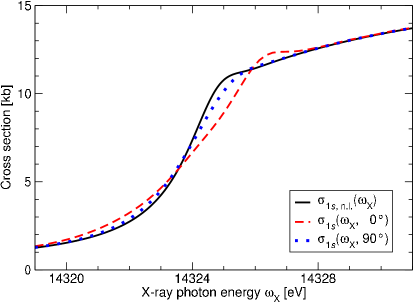
Figure 1: (Color online) X-ray photoabsorption cross section of the krypton atom near the $K$ edge with laser dressing $\sigma_{1s}(\omega_{\mathrm{X}},\vartheta_{\mathrm{LX}})$ and without it $\sigma_{1s,\mathrm{n.l.}}(\omega_{\mathrm{X}})$. The angle $\vartheta_{\mathrm{LX}}$ is formed between the polarization vectors of the laser and the x rays. The laser operates at a wavelength of $800\,{\rm{nm}}$ with an intensity of $10^{13}\,{\rm{W\over cm^{2}}}$.

The theory of the previous Sec. II shall now be applied to study the interaction of a krypton atom with two-color light. We use the Hartree-Fock-Slater code written by Herman and Skillman Herman and Skillman (1963), which has proven advantageous for atomic photoionization studies, e.g., Ref. Manson and Cooper, 1968, to determine the one-particle potential $V_{\mathrm{HFS}}(r)$ of krypton in Eq. (2). As in the original program of Herman and Skillman, the $X\alpha$ parameter is set to unity, in accordance with Ref. Slater, 1951. The radial equation (4) is solved using a representation of $u_{n,l}(r)$ in terms of $3001$ finite-element functions, which span a radial grid from $r_{\mathrm{min}}=0$ to $r_{\mathrm{max}}=60\,a_{0}$. For each of the orbital angular momentum quantum numbers $l=0,1,2,3$ considered, the lowest $100$ solutions were computed and used to form atomic orbitals (3) in the following; except in Fig. 3, where we use $500$ solutions to reproduce the high-energy behavior. In all cases, we verified that our results are converged with respect to the atomic basis set.

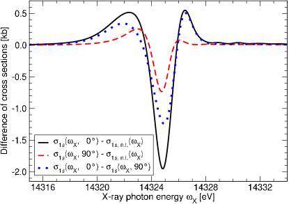
Figure 2: (Color online) Difference between x-ray photoabsorption cross sections of the krypton atom near the $K$ edge. Symbols as in Fig. 1.

The SES-CAP is constructed using the complex path (9). The path requires care when evaluated numerically due to the exponential functions therein. A complex scaling angle of $\theta=0.13\,{\rm{rad}}$ is used and the smoothness is $\lambda=5\,a_{0}^{-1}$. In our computations, the Hartree-Fock-Slater atomic potential assumes the long-range limit (1) to eight significant digits after $3\,a_{0}$, which defines the inner region of the krypton atom. We choose the exteriority $r_{0}=7\,a_{0}$, which ensures that the atomic ground state is unperturbed by the SES-CAP, as exploited in the derivation of Eq. (11).

The laser is assumed to operate with an optical wavelength of $800\,{\rm{nm}}$ (photon energy $1.55\,{\rm{eV}}$) and an intensity of $10^{13}\,{\rm{W\over cm^{2}}}$. The x-ray photon energy is varied in the vicinity of the $K$ edge of krypton, for which we use the experimental value $E_{1s}=-14327.17\,{\rm{eV}}$ of Breinig et al. Breinig et al. (1980). The experimental value for the decay width of a hole in the krypton $K$ shell is $\Gamma_{1s}=2.7$ eV Krause and Oliver (1979); Chen et al. (1980). To describe the laser dressing accurately, we have to include the photon blocks with $\mu=0,\pm 1,\ldots,\pm 5$ in the Floquet matrix (23).

IV Results and discussion

The x-ray photoabsorption cross section of krypton is plotted in Fig. 1 for three different cases: (a) The cross section without laser dressing, $\sigma_{1s,\mathrm{n.l.}}(\omega_{\mathrm{X}})$, (b) the cross section for parallel polarization vectors, denoted by $\sigma_{1s}^{\parallel}(\omega_{\mathrm{X}})$${}=\sigma_{1s}(\omega_{\mathrm{X}},0{}^{\circ})$, and (c) the cross section for perpendicular polarization vectors, denoted by $\sigma_{1s}^{\perp}(\omega_{\mathrm{X}})$${}=\sigma_{1s}(\omega_{\mathrm{X}},90{}^{\circ})$. Following Eq. (47), the chosen angles exhibit the largest effect of the polarization dependence of the cross section of the laser-dressed atom. The impact of the laser dressing is most clearly reflected in differences of the photoabsorption cross sections. They are shown in Fig. 2 for the cases $\sigma_{1s}^{\parallel}(\omega_{\mathrm{X}})$${}-{}$$\sigma_{1s,\mathrm{n.l.}}(\omega_{\mathrm{X}})$, $\sigma_{1s}^{\perp}(\omega_{\mathrm{X}})$${}-{}$$\sigma_{1s,\mathrm{n.l.}}(\omega_{\mathrm{X}})$, and $\sigma_{1s}^{\parallel}(\omega_{\mathrm{X}})$${}-{}$$\sigma_{1s}^{\perp}(\omega_{\mathrm{X}})$.

Inspecting Fig. 1, we see that, beginning a few electronvolts below the $K$ edge, the cross sections for laser on and off are smaller than $2\,{\rm{kb}}$. The reason for this is the fact that one is away from resonances for such x-ray energies because no one-photon excitation and ionization processes out of Kr$\,1s$ states are energetically allowed. Excitations or ionizations of higher lying shells, $L$, $M$, …, do not contribute noticeably in the energy range shown and are, therefore, not included in our theory.

Transition	$E_{\mathrm{HFS}}$ [eV]	$E_{\mathrm{expt}}$ [eV]
$1s\rightarrow 5p$	14324.81	14324.57
$1s\rightarrow 6p$	14326.01	14325.86
$1s\rightarrow 7p$	14326.48	14326.45
$1s\rightarrow 8p$	14326.75	14326.72

Table 1: Transition energies from the $K$ shell of krypton to Rydberg orbitals. Our results, $E_{\mathrm{HFS}}$, are obtained using the Hartree-Fock-Slater energies of the Rydberg orbitals $E_{\mathrm{Ryd}}$ in terms of the formula $E_{\mathrm{HFS}}=E_{\mathrm{Ryd}}-E_{1s}$, where $E_{1s}$ is the $K$-shell energy. The Hartree-Fock-Slater value for $E_{1s}$ is $E_{1,0}=-14022.88\,{\rm{eV}}$; it is replaced by the precise experimental value $-14327.17\,{\rm{eV}}$ Breinig et al. (1980). The experimental values $E_{\mathrm{expt}}$ are taken from Tab. 2 in Breinig et al. Breinig et al. (1980).

In the vicinity of the $K$ edge, there is an appreciable impact of the laser dressing on $\sigma_{1s}^{\parallel}(\omega_{\mathrm{X}})$ [Figs. 1 and 2]; it is suppressed with respect to the laser-free curve $\sigma_{1s,\mathrm{n.l.}}(\omega_{\mathrm{X}})$ between $\approx 14323\,{\rm{eV}}$ and $\approx 14326\,{\rm{eV}}$. Outside of this range, the cross section $\sigma_{1s}^{\parallel}(\omega_{\mathrm{X}})$ is somewhat larger than $\sigma_{1s,\mathrm{n.l.}}(\omega_{\mathrm{X}})$. Here, $\sigma_{1s}^{\perp}(\omega_{\mathrm{X}})$ behaves in a similar way, yet with a significantly lower deformation of the curve in relation to $\sigma_{1s,\mathrm{n.l.}}(\omega_{\mathrm{X}})$.

To understand this behavior we need to investigate the electronic structure in the vicinity of the ionization threshold first. Close to the threshold but still below are the energies for the transitions to Rydberg states. Exemplary Rydberg transition energies are listed in Tab. 1. Comparing the theoretical values to the experimental values, we find that the Hartree-Fock-Slater approximation describes the Rydberg orbitals, $5p$, $6p$, $7p$, and $8p$, accurately. This is attributed to the property of such orbitals to be very extended with only a small amplitude in the vicinity of the nucleus. Consequently, the one-particle approximation is very well justified. This reasoning is supported additionally by the observation that the agreement between theoretical and experimental energies in Tab. 1 increases with increasing principal quantum number of the Rydberg orbital involved.

Inspecting Tab. 1, we notice that the dip at $14324.82\,{\rm{eV}}$ ($14324.72\,{\rm{eV}}$) for the solid black (dashed red) curve lies very close to the energy of the $1s\to 5p$ Rydberg transition, i.e., to the energy of the final state which is a $1s^{-1}\,5p$ configuration. In a lowest order perturbation theoretical argument, emission of a laser photon from the $1s^{-1}\,5p$ configuration leads to the energy $14323.27\,{\rm{eV}}$ ($14323.37\,{\rm{eV}}$). It agrees with the energy of $1s^{-1}\,5s$ configuration, $14323.67\,{\rm{eV}}$. Conversely, the absorption of a laser photon from the $1s^{-1}\,5p$ configuration leads to $14326.37\,{\rm{eV}}$ ($14326.27\,{\rm{eV}}$), which is in the range of the energies of the $1s^{-1}\,4d$ and $1s^{-1}\,5d$ configurations, at $14325.61\,{\rm{eV}}$ and $14326.29\,{\rm{eV}}$, respectively. However, the coupling matrix elements between $5p$ and $5d$ and higher $d$ orbitals are small compared with the coupling of $5p$ and $4d$ orbitals. Hence, we conclude that the laser dressing causes a strong coupling of the $1s^{-1}\,5p$ configuration to the $1s^{-1}\,5s$ and $1s^{-1}\,4d$ configurations, which leads to the suppression of the $1s\to 5p$ transition and an enhancement around the energies of the $1s^{-1}\,5s$ and $1s^{-1}\,4d$ configurations.

Further above the $K$ edge, we see in Fig. 1 that the cross sections for laser on and off are essentially the same. Obviously, the relative importance of the energetic shift of the continuum of final states due to the laser dressing, the ponderomotive potential Freeman et al. (1988) $U_{\mathrm{p}}=2\pi\alpha{{I_{\mathrm{L}}}\over{\omega^{2}_{\mathrm{L}}}}=0.60\,{\rm{eV}}$, decreases for increasing x-ray photon energies. This is quantified by the quotient of $U_{\mathrm{p}}$ and the energy of the ejected electron. Clearly, the latter energy grows with increasing x-ray energy. In Fig. 2, above $14327.17\,{\rm{eV}}$, weak wiggles with the spacing of roughly the laser photon energy of $1.55\,{\rm{eV}}$ are observed.

The conservation of the integrated cross section (48) is proven under certain approximations in Sec. II.7. The applicability of this theorem can be examined by a numerical integration of the curves in Fig. 2 for $\omega_{\mathrm{X}}$ in the range $14300\,{\rm{eV}}$ to $14400\,{\rm{eV}}$. We obtain $-0.197\,{\rm{kb}}\,\,{\rm{eV}}$ (solid black), $-0.062\,{\rm{kb}}\,\,{\rm{eV}}$ (dashed red), and $-0.135\,{\rm{kb}}\,\,{\rm{eV}}$ (dotted blue). Following Sec. II.7, the resulting value—for an integration from $0$ to $\infty$—should be zero. To put these values in relation with the total deviation of the curves from zero, an integration of the absolute value of the curves is performed which yields $5.119\,{\rm{kb}}\,\,{\rm{eV}}$ (solid black), $1.534\,{\rm{kb}}\,\,{\rm{eV}}$ (dashed red), and $3.679\,{\rm{kb}}\,\,{\rm{eV}}$ (dotted blue). We find that the proportion of the integrated cross section to the integrated absolute value of the cross section is less than $-0.002$ for all curves. Hence the assumptions made in Sec. II.7 are fulfilled very well and the integrated cross section is essentially independent of the dressing-laser intensity.

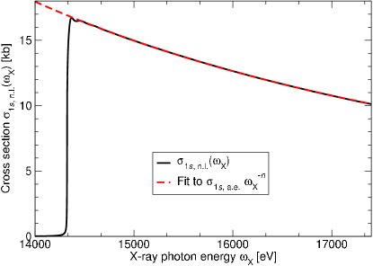
Figure 3: (Color online) Behavior of the photoabsorption cross section without laser $\sigma_{1s,\mathrm{n.l.}}(\omega_{\mathrm{X}})$ of the krypton atom above the $K$ edge. The data are fitted to the ansatz in Eq. (56), which gives $\sigma_{1s,\;\mathrm{a.e.}}=18623.8\,{\rm{kb}}\,\,{\rm{eV}}^{n}$ and $n=2.63$.

The photoabsorption cross section without laser $\sigma_{1s,\mathrm{n.l.}}(\omega_{\mathrm{X}})$ above the $K$ edge is displayed in Fig. 3 for a larger range of x-ray energies than in Fig. 1. The overall shape of our curve resembles the experimental result in Fig. 1 of Schaphorst et al. Schaphorst et al. (1993). However, our curve does not reach the same peak height of $\approx 19\,{\rm{kb}}$ and it rises less steeply [our Fig. 1]. Considering the one-particle model adopted here, the agreement is satisfactory. The photoabsorption cross section of hydrogen atoms above the $K$ edge is described by a simple formula, e.g., Ref. Bethe and Salpeter, 1957,

$$\sigma_{1s}(\omega_{\mathrm{X}})=\sigma_{1s,\;\mathrm{a.e.}}\>\omega_{\mathrm{X}}^{-n}\;.$$ (56)

For hydrogen, the exponent is $n=8/3=2.\bar{6}$ in the vicinity of the edge, i.e., where the ejected electrons only have a small fraction of the $K$-shell energy. It rises to the well-known $n=7/2=3.5$ far away from the edge for values of $\omega_{\mathrm{X}}$ that are 100 times or more the $K$ shell energy Bethe and Salpeter (1957). Formula (56) can be expected to well approximate the $K$-shell photoabsorption cross section of more complex atoms like krypton Bethe and Salpeter (1957). We obtain the constants $\sigma_{1s,\;\mathrm{a.e.}}=18623.8\,{\rm{kb}}\,\,{\rm{eV}}^{n}$ and $n=2.63$ for the above-edge behavior of the cross section in Eq. (56) by a nonlinear curve fit Moré (1977) of the data in Fig. 3. The exponent $n$ is very close to the value derived for hydrogen, which corroborates the assumption that also the above-edge behavior of the Kr$\,1s$ cross section is well described by the theory and methods presented in this paper. Moreover, $n$ is consistent with a fit to the experimental attenuation cross section of krypton in Ref. Saloman et al., 1988 in the respective energy range.

V Conclusion

We derive a formula for the x-ray photoabsorption cross section of an atom in the light of a medium-intensity laser in the optical wavelength regime. The laser and the x rays are assumed to be linearly polarized. The dressing laser effects a modification of the near-edge x-ray absorption and a polarization dependence of the absorption cross section on the angle between the electric field vectors of the individual light sources.

We use the Hartree-Fock-Slater approximation to describe the atomic many-particle problem in conjunction with a nonrelativistic quantum-electrodynamic approach to treat the light-electron interaction. In order to deal with continuum electrons, a complex absorbing potential is employed that is derived using the smooth exterior complex scaling technique. Using the atomic orbitals and the number states of the free electromagnetic fields in a product basis, a two-mode (or two-color) matrix representation of the Hamiltonian is calculated. A direct diagonalization of the complex symmetric matrix leads to the transition rates for excitation out of the $K$ shell, which are used to calculate the cross section. Due to the relatively low intensity of existing third-generation synchrotron sources, x-ray absorption may be described by a one-photon process. This property is exploited in terms of a perturbative treatment to simplify the two-mode problem, using both time-independent and time-dependent derivations of the formula for the cross section. The angular dependence of the cross section is studied and the approximate conservation of its integral from 0 to $\infty$ is proven.

The theory is applied to a single krypton atom near the $K$ edge. A pronounced modification of the energy-dependent cross section is found with laser dressing. The modification of the cross section depends notably on the angle between the polarization vectors of laser and x rays. The behavior of the cross section above the edge is found to follow a well-known approximation, thus reassuring the usefulness and quality of the theoretical framework. Our theoretical predictions for noble-gas atoms (see also Ref. Buth et al., 2007) are presently under experimental investigation.

Our studies offer motivation and prospects for future research. The theoretical framework of this article can easily be extended to multiphoton x-ray processes for the emerging x-ray free electron lasers, e.g., the Linac Coherent Light Source (LCLS) Arthur et al. (2002) at the Stanford Linear Accelerator Center (SLAC). Further investigations should treat the dependence of the photoabsorption cross section on the wavelength and intensity of the laser. Moreover, we used the electric dipole approximation in our derivations. We expect nondipole effects to cause deviations from the angular dependence of our formula for the total photoabsorption cross section. This proposed route to study such effects is in fact much easier than the conventional way to measure angular distributions of photoelectrons. Furthermore, improvements of the description of the atomic many-particle problem offer intriguing perspectives to study the interaction of light with correlated electrons and the competition between the strength of both interactions.