Accuracy of Sampling Quantum Phase Space in Photon Counting Experiment
Abstract
We study the accuracy of determining the phase space quasidistribution of a single quantized light mode by a photon counting experiment. We derive an exact analytical formula for the error of the experimental outcome. This result provides an estimation for the experimental parameters, such as the number of events, required to determine the quasidistribution with assumed precision. Our analysis also shows that it is in general not possible to compensate the imperfectness of the photodetector in a numerical processing of the experimental data. The discussion is illustrated with Monte Carlo simulations of the photon counting experiment for the coherent state, the one photon Fock state, and the Schrödinger cat state.
PACS number(s): 42.50.Dv, 42.50.Ar
I Introduction
Generation and detection of simple quantum systems exhibiting nonclassical features have been, over the past few years, a subject of numerous experimental and theoretical studies. Quantum optics, provides in a natural way, several interesting examples of nonclassical systems along with practical tools to perform measurements. One of the simplest systems is a single quantized light mode, whose Wigner function has been measured in a series of beautiful experiments using optical homodyne tomography [2, 3] following a theoretical proposal [4].
Recently, a novel method for the determination of the Wigner function of a light mode has been proposed [5, 6]. This method utilizes a direct relation between the photocount statistics and the phase space quasidistributions of light. Simplicity of this relation makes it possible to probe independently each point of the single mode phase space. In a very recent experiment, an analogous method has been used to measure the Wigner function of the motional state of a trapped ion [7].
In the present paper we supplement the description of this method with a rigorous analysis of the statistical uncertainty, when the phase space quasidistribution is determined from a finite sample of measurements. The analysis of the reconstruction errors due, for example, to a finite set of recorded photons is essential in designing an experiment that can provide accurate reconstruction of the phase space quasidistribution. We will derive analytical formulae for the uncertainty of the experimental result, which give theoretical control over the potential sources of errors. Additional motivation for these studies comes from recent discussions of the possibility of compensating the detector losses in quantum optical measurements [8, 9]. Our analysis will provide a detailed answer to the question whether such a compensation is possible in the newly proposed scheme.
This paper is organized as follows. First, in Sec. II we briefly review properties of the quasidistribution functions that are relevant to the further parts of the paper. Then, in order to make the paper self–contained, we present the essentials of the method in Sec. III. Next we derive and discuss the statistical error of the experimentally determined quasidistribution in Sec. IV. The general results are illustrated with several examples in Sec. V. Finally, Sec. VI summarizes the paper.
II Quasidistributions of a single light mode
The phase space representation of the state of a single quantized light mode as a function, of one complex variable , has been extensively used in quantum optics since its very beginning. Due to the noncommutativity of the boson creation and annihilation operators, the Wigner function is just an example of the more general -parameterized quasiprobability distributions. Such a one–parameter family of quasidistribution functions is given by the following formula [10]:
| (1) |
where and are the single mode photon annihilation and creation operators, and the real parameter defines the corresponding phase space distribution. It is well known that such a parameter is associated with the ordering of the field bosonic operators. For example, and correspond to the normal, symmetric and antinormal ordering, respectively. The corresponding quasidistributions are: the function, the Wigner function, and the function. The properties of the -parameterized quasiprobability distributions are quite different. For example: the function is highly singular for nonclassical states of light, the Wigner function is well behaved for all states, but may take negative values, and finally the function is always positive definite. These properties reflect a general relation linking any two differently ordered quasidistributions via convolution with a Gaussian function in the complex phase space:
| (2) |
where . Thus the lower the ordering, the smoother the quasidistribution is, and fine details of the functions are not easily visible.
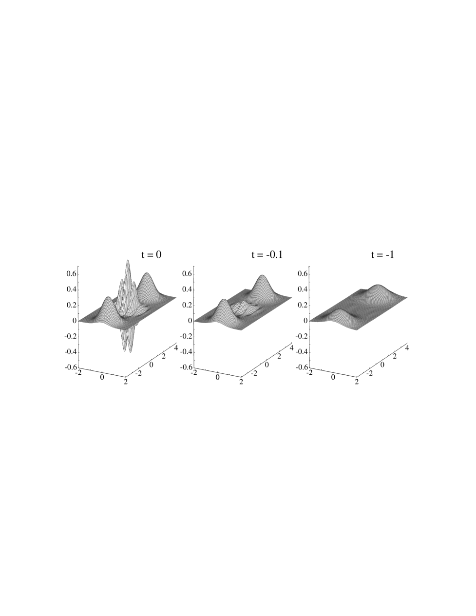
This behavior can be explicitly illustrated using a superposition of two coherent states:
| (3) |
States of this type illustrate quantum coherence and interference between classical–like components, and are often called quantum optical Schrödinger cats [4, 11]. The quasidistribution of this superposition is given by the formula
| (5) | |||||
Fig. 1 shows this quasidistribution plotted for three different values of the ordering parameter . The Wigner function contains an oscillating component originating from the interference between the coherent states. This component is completely smeared out in the function, which can hardly be distinguished from that of a statistical mixture of two coherent states.
Computation of a higher ordered quasidistribution from a given one is not a straightforward task, since the integral in Eq. (2) fails to converge for . Instead, a relation linking the Fourier transforms of the quasidistributions can be used in analytical calculations:
| (6) |
However, its application in the processing of experimental data would enormously amplify the statistical error [12]. Consequently, in the case of experimentally determined functions it is practically impossible to compute a higher ordered quasidistribution from the measured one. Therefore the ordering of the measured quasidistribution depends primarily on the features of a specific experimental scheme. Optical homodyne tomography is capable of measuring the Wigner function, provided that the detection is lossless. For heterodyne [13] and double homodyne [14] detection schemes the function is the limit, because in these methods an additional noise is introduced by a vacuum mode mixed with the detected fields.
In our calculations a normally ordered representation of the quasidistribution functions will be very useful. Introducing normal ordering of the creation and annihilation operators in Eq. (1) allows to perform the integral explicitly, which yields:
| (7) |
This formula can be transformed into the form [15]:
| (8) |
showing that for the quasidistribution is an expectation value of a bounded operator and therefore is well behaved. Of course, only well behaved, nonsingular functions have experimental significance.
III Photocount statistics and quasidistributions
The experimental setup proposed to determine the quasiprobability distribution via photon counting is presented in Fig. 2. The signal, characterized by an annihilation operator is superposed by a beam splitter on a probe field prepared in a coherent state . The measurement is performed only on one of the output ports of the beam splitter, delivering the transmitted signal mixed with the reflected probe field. The quantity detected on this port is simply the photon statistics, measured with the help of a single photodetector. We will consider an imperfect detector, described by a quantum efficiency . According to the quantum theory of photodetection, the probability of registering counts by the detector is given by the expectation value of the following normally ordered operator:
| (9) |
where the angular brackets denote the quantum expectation value and is the operator of the time–integrated flux of the light incident onto the surface of the detector. It can be expressed in terms of the signal and probe fields as
| (10) |
with being the beam splitter power transmission. The count statistics determined in the experiment is used to compute the following photon count generating function (PCGF):
| (11) |
where is a real parameter, which will allow us to manipulate to some extent the ordering of the measured phase space quasidistribution. We will specify the allowed range of the parameter later. A comparison of the latter form of the PCGF with Eq. (7) shows that it is directly related to a specifically ordered quasidistribution of the signal field. After the identification of the parameters we obtain that the PCGF can be written as:
| (12) |
Thus the PCGF computed from the count statistics is proportional to the value of the signal quasiprobability distribution at the point , determined by the amplitude and the phase of the probe coherent field [16]. We may therefore scan the whole phase space of the signal field by changing the parameters of the probe field. The main advantage of this scheme is that the measurement of the quasidistribution is performed independently at each point of the phase space. In contrast to optical homodyne tomography there is no need to gather first the complete set of experimental data and then process it numerically.
The ordering of the measured quasidistribution depends on two quantities: the parameter used in the construction of the PCGF from the count statistics, and the product of the beam splitter transmission and the detector efficiency . Let us first consider the case of an ideal detector and the transmission tending to one. In this limit the ordering of the quasidistribution approaches . Setting , which corresponds to multiplying the count statistics by , yields the Wigner function of the signal field. However, in the limit only a small fraction of the probe field is reflected to the detector, which results in the vanishing factor multiplying in Eq. (12), and thus an intense probe field has to be used to achieve the required shift in the phase space. Consequently, the beam splitter should have the transmission close to one, yet reflect enough probe field to allow scanning of the interesting region of the phase space. This decreases the ordering of the measured quasidistribution slightly below zero. A more important factor that lowers the ordering is the imperfectness of the detector. Maximum available efficiency of photodetectors is limited by the current technology and on the level of single photon signals does not exceed 80% [17]. Therefore in a realistic setup the parameter deciding about the magnitude of the product is the detector efficiency rather then the beam splitter transmission.
One may attempt to compensate the lowered ordering by setting , which would allow to measure the Wigner function regardless of the value of . However in this case the magnitude of the factor multiplying the count statistics in the PCGF diverges to infinity, which would be a source of severe problems in a real experiment. We will discuss this point in detail later, in the framework of a rigorous statistical analysis of the measurement.
Let us close this section by presenting several examples of the photocount statistics for different quantum states of the signal probed by a coherent source of light. The most straightforward case is when a coherent state enters through the signal port of the beam splitter. Then the statistics of the registered counts is given by the Poisson distribution:
| (13) |
where is the average number of registered photons. When the measurement is performed at the point where the quasidistribution of the signal field is centered, i.e., , the fields interfere destructively and no photons are detected. In general, for an arbitrary phase space point, the average number of registered photons is proportional to the squared distance from . Averaging Eq. (13) over an appropriate representation yields the photocount statistics for a thermal signal state characterized by an average photon number :
| (15) | |||||
where denotes the th Laguerre polynomial.
A more interesting case is when the signal field is in a nonclassical state. Then the interference between the signal and the probe fields cannot be described within the classical theory of radiation. We will consider two nonclassical states: the one photon Fock state and the Schrödinger cat state. The count statistics can be obtained by calculating the quantum expectation value of PCGF over the considered state and then expanding it into the powers of .
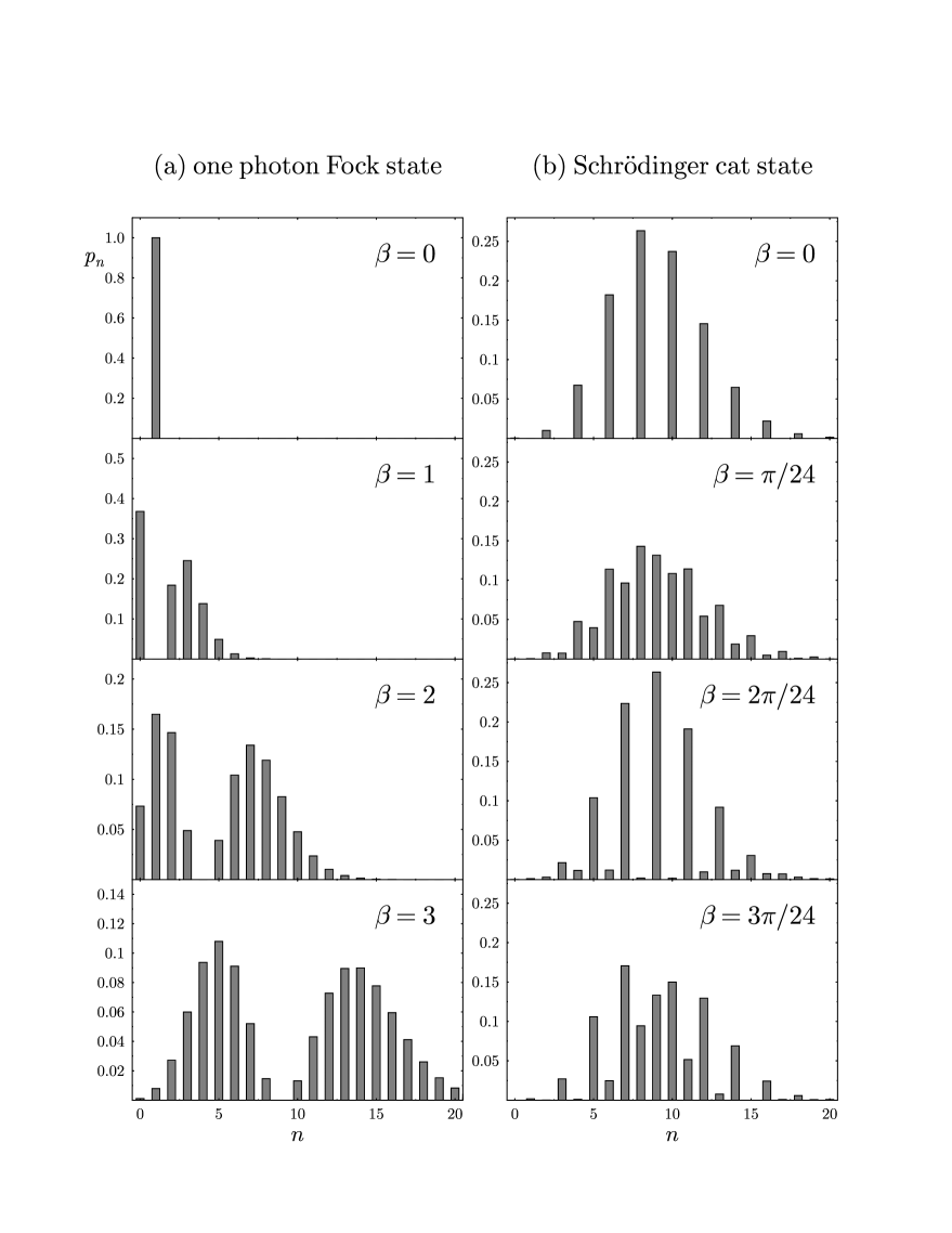
The photocount distribution for the one photon Fock state can be written as an average of two terms with the weights and :
| (17) | |||||
The second term corresponds to the detection of the vacuum signal field. Its presence is a result of the detector imperfectness and the leakage of the signal field through the unused output port of the beam splitter. This term vanishes in the limit of , where the Wigner function is measured in the setup. The first term describes the detection of the one photon Fock state. In Fig. 3(a) we show the statistics generated by this term for different values of . If the amplitude of the probe field is zero, we detect the undisturbed signal field and the statistics is nonzero only for . The distribution becomes flatter with increasing . Its characteristic feature is that it vanishes around .
For the Schrödinger cat state defined in Eq. (3) the photocount statistics is a sum of three terms:
| (19) | |||||
The first two terms describe the two coherent components of the cat state, whereas the last one contributes to the quantum interference structure. In Fig. 3(b) we plot the photocount statistics for different values of probing this structure, in the limit . The four values of correspond to the cosine function in Eq. (5) equal to and , respectively, for . It is seen that the form of the statistics changes very rapidly with . This behavior becomes clear if we rewrite the PCGF (Eq. (11)) for in the form
| (20) |
showing that in order to obtain a large positive (negative) value of the quasidistribution the photocount statistics has to be concentrated in even (odd) values of .
IV statistical error
The proposed measurement scheme is based on the relation between the quasidistributions and the photocount statistics. In a real experiment the statistics of the detector counts cannot be known with perfect accuracy, as it is determined from a finite sample of measurements. This statistical uncertainty affects the experimental value of the quasidistribution. Theoretical analysis of the statistical error is important for two reasons. First, we need an estimation for the number of the measurements required to determine the quasidistribution with a given accuracy. Secondly, we have seen that one may attempt to compensate the imperfectness of the detector and the nonunit transmission of the beam splitter by manipulating the parameter . However, in this case the magnitude of the factor multiplying the count statistics diverges to infinity. This amplifies the contribution of the tail of the distribution, which is usually determined from a very small sample of data, and may therefore result in a huge statistical error of the final result. Our calculations will provide a quantitative analysis of this problem.
Due to extreme simplicity of Eq. (11), linking the count statistics with the quasidistributions, it is possible to perform a rigorous analysis of the statistical error and obtain an exact expression for the uncertainty of the final result. We will assume that the maximum number of the photons that can be detected in a single measurement cannot exceed a certain cut–off parameter . Let us denote by the number of measurements when photons have been detected, . The set of ’s obeys the multinomial distribution
| (22) | |||||||
The measured count statistics is converted into the experimental PCGF:
| (23) |
which is an approximation of the series defined in Eq. (11). In order to see how well approximates the ideal quantity we will find its mean value and its variance averaged with respect to the distribution (22). This task is quite easy, since the only expressions we need in the calculations are the following moments:
| (24) | |||||
| (25) |
We use the bar to denote the statistical average with respect to the distribution . Given this result, it is straightforward to obtain:
| (26) |
and
| (27) | |||||||
| (28) | |||||||
The error introduced by the cut–off of the photocount statistics can be estimated by
| (30) | |||||
| (31) |
The variance is a difference of two terms. The second one is simply the squared average of . The first term is a sum over the count statistics multiplied by the powers of a positive factor . If , this factor is greater than one and the sum may be arbitrarily large. In the case when the contribution from the cut tail of the statistics is negligible, i.e., if , it can be estimated by the average number of registered photons:
| (32) |
Thus, the variance grows unlimited as we probe phase space points far from the area where the quasidistribution is localized. Several examples in the next section will demonstrate that the variance usually explodes much more rapidly, exponentially rather than linearly. This makes the compensation of the detector inefficiency a very subtle matter. It can be successful only for very restricted regions of the phase space, where the count statistics is concentrated for a small number of counts and vanishes sufficiently quickly for larger ’s.
Therefore, in order to ensure that the statistical error remains bounded over the whole phase space, we have to impose the condition . Since we are interested in achieving the highest possible ordering of the measured quasidistribution, we should consequently set . For this particular value the estimations for the uncertainty of take a much simpler form. The error caused by the cut–off of the count distribution can be estimated by the “lacking” part of the probability:
| (33) |
which shows that the cut–off is unimportant as long as the probability of registering more than photons is negligible. The variance of is given by
| (34) | |||||
| (35) |
Thus, the statistical uncertainty of the measured quasidistribution can be simply estimated as multiplied by the proportionality constant given in Eq. (12). It is also seen that the uncertainty is smaller for the phase space points where the magnitude of the quasidistribution is large.
Analysis of the statistical error for the recently demonstrated measurement of the Wigner function of a trapped ion is different, as the analog of is not determined by a counting–like method [18]. A quantity that is detected in the experimental setup is the time–dependence of the fluorescence light produced by driving a selected transition. This signal is a linear combination of the populations of the trap levels with known time–dependent coefficients, and the ’s are extracted from these data by solving the resulting overdetermined set of linear equations. Consequently, their statistical error is not described by a simple analytical formula. Additional source of error is the uncertainty of the phase space displacement, which is performed by applying an rf field. An element of our analysis that can be directly transferred to the case of a trapped ion is the effect of the cut–off of the count statistics.
V Examples
We will now consider several examples of the reconstruction of the quasidistributions from the data collected in a photon counting experiment. Our discussion will be based on Monte Carlo simulations compared with the analytical results obtained in the previous section.
First, let us note that the huge statistical error is not the only problem in compensating the detector inefficiency. If , the sum (26) does not even have to converge in the limit of . An example of this pathological behavior is provided by a thermal state, which has been calculated in Eq. (15). For the zero probe field we obtain
| (36) |
which shows that if , then for a sufficiently intense thermal state the magnitude of the summand is larger than one and consequently the sum diverges, when . This behavior is due to the very slowly vanishing count distribution and it does not appear for the other examples of the count statistics derived in Sec. III.
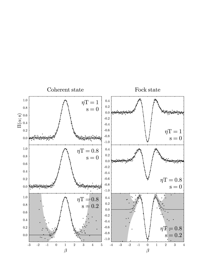
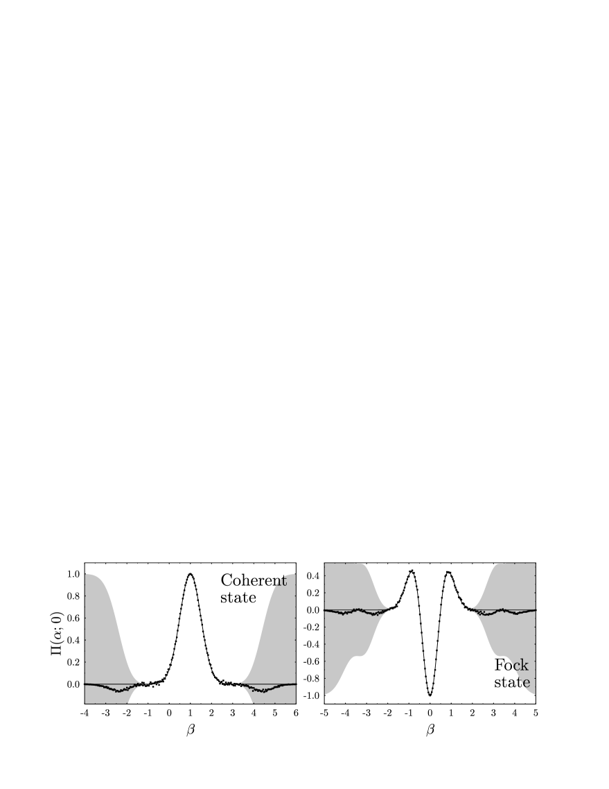
In Fig. 4 we plot the reconstructed quasidistributions for the coherent state and the one photon Fock state. Due to the symmetry of these states, it is sufficient to discuss the behavior of the reconstructed quasidistribution on the real axis of the phase space. The cut–off parameter is set high enough to make the contribution from the cut tail of the statistics negligibly small. The quasidistributions are determined at each phase space point from the Monte Carlo simulations of events. The grey areas denote the statistical uncertainty calculated according to Eq. (LABEL:Eq:PiexpDispersion). The two top graphs show the reconstruction of the Wigner function in the ideal case . It is seen that the statistical error is smaller, where the magnitude of the Wigner function is large. In the outer regions it approaches its maximum value . The effect of the nonunit is shown in the center graphs. The measured quasidistributions become wider and the negative dip in the case of the Fock state is shallower. In the bottom graphs we depict the result of compensating the nonunit value of by setting . The compensation works quite well in the central region, where the average number of detected photons is small, but outside of this region the statistical error explodes exponentially. Of course, the statistical error can be suppressed by increasing the number of measurements. However, this is not a practical method, since the statistical error decreases with the size of the sample only as .
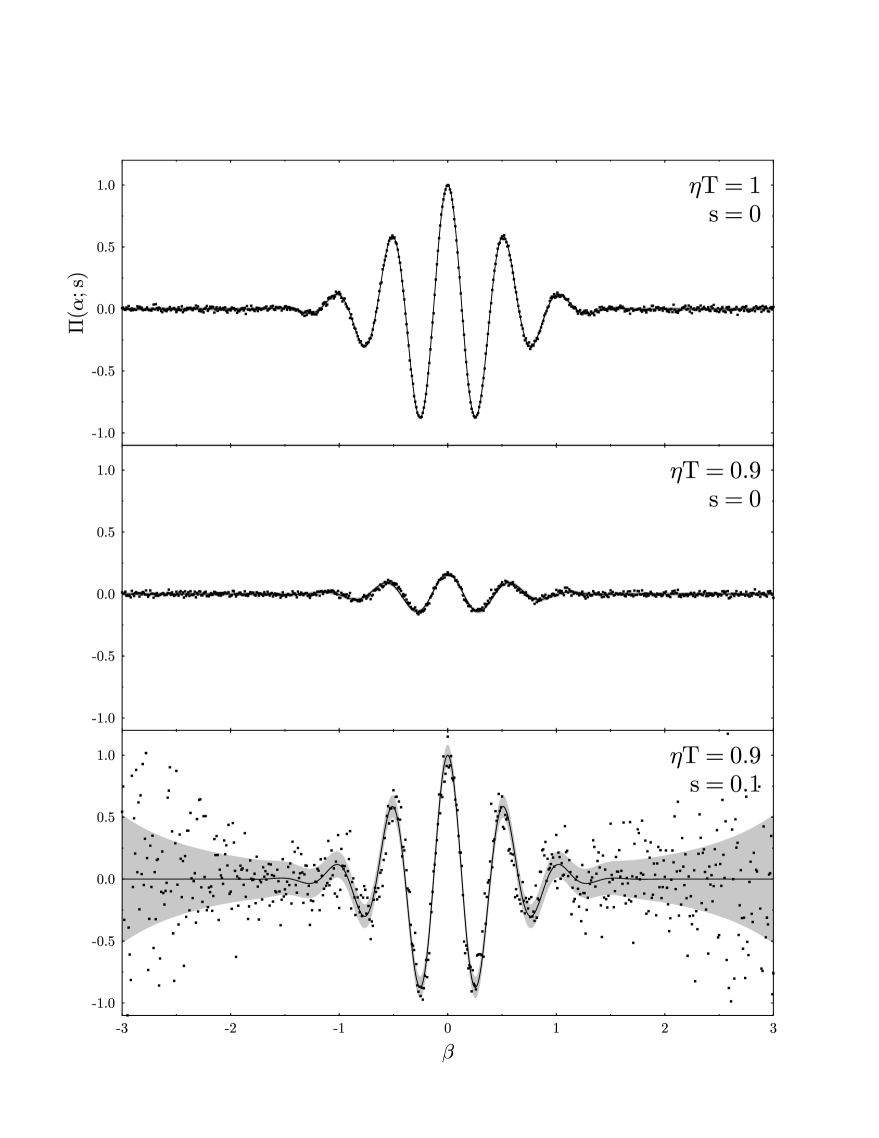
The reconstruction of the interference structure of the Schrödinger cat state is plotted in Fig. 5. This structure is very fragile, and its precise measurement requires a large sample of events. In the case of the presented plot, simulations were performed at each phase space point. Comparison of the top and the center graphs shows how even a small imperfectness in the detection destroys the interference pattern. The data collected in an nonideal setup can be processed to recover the Wigner function, but at the cost of a significantly larger statistical error, as it is shown in the bottom graph. Outside the interference structure, we again observe the exponential explosion of the dispersion due to the increasing intensity of the detected light.
Finally, let us look at the effect of cutting the statistics at a finite value. Fig. 6 shows the Wigner functions for the one photon coherent and Fock states reconstructed from the count distributions cut at . We performed a large number of simulations in order to get the pure effect of the cut–off that is not spoiled by the statistical uncertainty. The grey areas show the cut–off error, estimated using Eq. (33). The reconstruction works well as long as the probability of detecting more than photons is negligible. When the average number of incident photons starts to be comparable with the cut–off parameter, “ghost” peaks appear. When we go even further, the Wigner function again tends to zero, but this is a purely artificial effect due to the virtually vanishing count distribution below .
VI Conclusions
The newly proposed scheme for measuring the quasiprobability distributions is based on a much more direct link with the data collected in an experiment than optical homodyne tomography. Furthermore, each point of the phase space can be probed independently. The simplicity of the underlying idea allowed us to discuss rigorously the experimental issues, such us the statistical uncertainty and the effect of the cut–off of the count statistics.
We have seen that it is, in general, not possible to compensate the detector inefficiency. This conclusion may seem to be surprising, since it was shown that the true photon distribution can be reconstructed from photocount statistics of an imperfect detector, provided that its efficiency is larger that 50% [9]. Moreover, a simple calculation shows that an application of this recipe for recovering the photon distribution is equivalent to setting the parameter above zero. The solution of this seeming contradiction is easy: the proposed recipe can be safely used as long as we are interested in the photon statistics itself. However, the statistical errors of the reconstructed probabilities are not independent, and an attempt to utilize these probabilities to calculate another physical quantity may lead to accumulation of the statistical fluctuations and generate a useless result. The simple alternating series is an example of such a quantity.
Acknowledgments
This work has been partially supported by the Polish KBN grant 2 PO3B 006 11. K.B. thanks the European Physical Society for the EPS/SOROS Mobility Grant.
REFERENCES
- [1] Permanent address: Instytut Fizyki Teoretycznej, Uniwersytet Warszawski, Hoża 69, PL–00–681 Warszawa, Poland.
- [2] D. T. Smithey, M. Beck, M. G. Raymer, and A. Faridani, Phys. Rev. Lett. 70, 1244 (1993); D. T. Smithey, M. Beck, J. Cooper, M. G. Raymer, and A. Faridani, Phys. Scr. T48, 35 (1993).
- [3] G. Breitenbach, T. Müller, S. F. Pereira, J.-Ph. Poizat, S. Schiller, and J. Mlynek, J. Opt. Soc. Am. B 12, 2304 (1995).
- [4] K. Vogel and H. Risken, Phys. Rev. A 40, R2847 (1989).
- [5] S. Wallentowitz and W. Vogel, Phys. Rev. A 53, 4528 (1996).
- [6] K. Banaszek and K. Wódkiewicz, Phys. Rev. Lett. 76, 4344 (1996).
- [7] D. Leibfried, D. M. Meekhof, B. E. King, C. Monroe, W. M. Itano, and D. J. Wineland, Phys. Rev. Lett. (to be published).
- [8] G. M. D’Ariano, U. Leonhardt, and H. Paul, Phys. Rev. A 52, R1801 (1995).
- [9] T. Kiss, U. Herzog, and U. Leonhardt, Phys. Rev. A 52, 2433 (1995).
- [10] K. E. Cahill and R. J. Glauber, Phys. Rev. 177, 1882 (1969).
- [11] W. Schleich, M. Pernigo, and F. Le Kien, Phys. Rev. A 44, 2172 (1991); for a review see V. Bužek and P. L. Knight, in Progress in Optics XXXIV, ed. by E. Wolf (North-Holland, Amsterdam, 1995).
- [12] U. Leonhardt and H. Paul, Phys. Rev. Lett. 72, 4086 (1994); J. Mod. Opt. 41, 1427 (1994).
- [13] J. H. Shapiro and S. S. Wagner, IEEE J. Quantum Electron. QE-20, 803 (1984).
- [14] N. G. Walker, J. Mod. Opt. 34, 15 (1987); M. Freyberger and W. Schleich, Phys. Rev. A 47, R30 (1993); U. Leonhardt and H. Paul, Phys. Rev. A 47, R2460 (1993).
- [15] B.-G. Englert, J. Phys. A: Math. Gen. 22, 625 (1989).
- [16] In the limit the PCGF provides a representation of the quasidistributions as a series in terms of displaced number states, which has been derived by H. Moya-Cessa and P. L. Knight, Phys. Rev. A 48, 2479 (1993).
- [17] P. G. Kwiat, A. M. Steinberg, R. Y. Chiao, P. H. Eberhard, and M. D. Petroff, Phys. Rev. A 48, R867 (1993).
- [18] D. M. Meekhof, C. Monroe, B. E. King, W. M. Itano, and D. J. Wineland, Phys. Rev. Lett. 76, 1796 (1996).