Coherent Nonlinear Phenomena in High Energy Synchrotrons:
Observations and Theoretical Models

Abstract

Nonlinear waves have been observed in synchrotrons for years but have received little attention in the literature. While pathological, these phenomena are worth studying on at least two accounts. First, the formation of solitary waves may lead to droplet formation that causes significant beam halo to develop. It is important to understand the conditions under which such behavior may be expected in terms of the machine impedance. Secondly, a variety of nonlinear processes are likely involved in the normal saturation of unstable oscillations, leading to the possibility that low-level, but potentially broadband fluctuation spectra may develop. The resulting fluctuation spectra carry indirectly the signature of the machine impedance. In this work we review a number of observations of nonlinear longitudinal waves made in Fermilab accelerators, and make a first attempt to develop appropriate theoretical models to explain these observations.

1 Introduction

Over the years, nonlinear wave phenomena have received scant attention in high energy synchrotrons, in part, because of the mathematical difficulty of this subject, but also due to the fact that nonlinear wave motion is usually associated with a pathological state of an accelerator that is best to be avoided. While this is indeed true for the most violent nonlinear effects, a broad class of low-level processes may be playing a role in many present machines, and the drive for ever higher beam intensities may lead to the widespread occurrence of nonlinear wave phenomena.

In particular, in the case of the dynamical behavior in the vicinity of an intense, stored beam, we are interested in the formation of beam halo, either as a diffuse cloud, represented by a departure from a Gaussian distribution, or as droplets which may occur in a type of phase transition at beam’s edge due to coherent modes. In addition, it is useful to study the formation of an equilibrium state, if it exists, between a broad spectrum of marginally stable modes and some weak dissipative mechanisms that can lead to a saturated state of low-level turbulence, which, in turn, can affect the rate at which the halo population is generated. These phenomena can be expected to be most prevalent in hadron rings owing to the weakness of the damping mechanisms, and our attention in this paper is focussed on this case.

While these subjects are mathematically complex, a rich literature already exists in the field of plasma physics that deals with these questions, although the interparticle force predominantly considered in this literature is due to space charge alone. At the relativistic energies typical in modern accelerators, the interaction between particles is dominated by wall image currents, i.e. the wakefields, which complicates the nature of the interaction, but can also lead to a wider variety of wave phenomena. It is our aim in this work to highlight observations of nonlinear wave phenomena in high-energy synchrotrons and to point out methods of analysis from plasma physics that can be applied to the study of these topics.

The types of wave behavior in beams may be classified according to the degree of nonlinearity, in parallel with the concepts in plasma physics. In the linear regime, a resonant mode can be driven resulting in a response at the drive frequency which is characteristic of the beam intensity and the nature of the wakefield, or impedance, of the machine. When detected by a suitable pick-up, the driven response can shed light on the properties of the wakefields and the proximity of the beam to the stability threshold. This socalled transfer function method [1] is widely used to study accelerator stability.

If an accelerator is operated just above its stability limit, the most unstable mode is driven into exponential growth by the wakes, reaching a saturated, though marginally stable, state as the beam distribution is altered by the growing waves. If the spectrum of unstable modes is sufficiently broad, the phase of the perturbation is effectively random, and the interaction of waves and particles leads to particle diffusion in phase space, known in plasma physics as quasi-linear diffusion [2]. The analog in beams, known as the ’overshoot’ phenomenon, has been studied [3],[4], although the applicability of this model is unclear owing to the typically narrow unstable spectrum found in many storage rings. A recent numerical study of this phenomenon that shows the complexity of the interaction is found in ref. [5].

However, particularly in hadron rings where the absence of synchrotron damping allows virtually unimpeded mode growth, unstable waves can grow to finite amplitudes that permit a significant fraction of the beam to become trapped in its own wake. The resulting wave motion couples to the trapped particles in such a way as to give rise to slowly damped oscillations. This phenomenon is known as nonlinear Landau damping in the plasma physics literature [6] (in comparison to linear Landau damping which is part of the linear beam response). It is to be expected that where a discrete spectrum of unstable waves can occur, as is often the case in a synchrotron, that nonlinear Landau damping can play an important role.

At the next higher level of nonlinear interaction, coherent modes can resonantly interact in a process known as the three- wave interaction [7]. This leads typically to a cascade in frequency which, due to the harmonic character of many modes in storage rings, readily occurs and can cause a broadening of the original unstable spectrum. This phenomenon has been studied in the simple case of longitudinal oscillations in a coasting beam, [8] and it can be expected that similar wave-wave coupling can occur in the transverse plane and in bunched beams as well, albeit with different resonance conditions.

If the coherent motion is particularly violent, and sufficiently dissipative, then the trapped portion of the beam can self-extract from the core of the beam distribution, forming droplets at the beam edge that can be self-sustaining. These are, presumably, a form of solitary wave, or soliton, which is perhaps unique to a high-energy synchrotron due to the complex character of the wake field. Such solitary waves may be a primary producer of halo particles for weakly-damped hadron rings.

In general, we are interested in the final state of these various nonlinear interactions: the condition where the coherent modes reach marginal stability through either a change in the beam distribution, or through frequency spreading of the spectral distribution. In the latter case, the phonons themselves can be thought of as comprising a fluid which comes into equilibrium, the details of which depend on the inter-phonon interaction. In the plasma physics literature, scaling laws for the resulting turbulent fluctuation spectrum have been derived ([9] and references contained therein). For our purposes, we would like to understand how aspects of the machine impedance, and therefore the detailed design, contribute to the form of the equilibrium turbulent spectrum, if it exists.

In this paper we review the observations made at Fermilab [8] in stored high energy hadron beams and compare the observations with numerical simulations. Our experimental studies, and thus our theoretical work, have been focussed on the phenomena in perhaps the simplest of all cases, that of longitudinal oscillations of a coasting, or unbunched, beam in a storage ring. As such, the surface of this subject has only been scratched, and our aim here is to outline the steps that would have to be taken to study any of the many other possible situations where nonlinear waves can occur. Moreover, we would like to underscore the importance of understanding turbulence in beams that we feel will be playing an increasingly important role as beams are more commonly run close to, or even above, their linear stability boundaries.

2 Review of Basic Phenomena

2.1 Stability in Particle Beams

In the case of a high-energy stored beam, the growth of coherent wave motion is normally undesireable. Wakefields can drive such waves, though the mode growth is counteracted by damping due to the spread in frequencies of the individual particles making up the beam, and this damping effect was first derived for a plasma, known as Landau damping [10]. A well known technique for determining the linear stability boundary of a beam is to excite driven oscillations on the beam and to monitor the amplitude and phase of the beam’s response, which includes the effects of wakefields. This technique, known as a beam transfer function, [1], yields for longitudinal motion in a coasting beam a response of the form

$$R(\Omega)=\frac{1}{\frac{i(e\omega_{s})^{2}}{2\pi}\int_{-\infty}^{\infty}\frac{\frac{\partial f_{o}}{\partial\epsilon}}{\Omega-m(\omega_{s}+k_{o}\epsilon)}d\epsilon}+Z(\Omega)$$ (1)

where $\omega_{s}$ is the harmonic revolution frequency, $f_{o}$ is the longitudinal particle distribution function, $\varepsilon$ is the energy deviation, $k_{o}$ is the frequency dispersion factor and $Z(\Omega)$ is the machine impedance. This function is directly related to the dispersion relation for longitudinal modes given by

$$D_{m}(\Omega)=1+Z(\Omega)\frac{i(e\omega_{s})^{2}}{2\pi}\int_{-\infty}^{\infty}\frac{\frac{\partial f_{o}}{\partial\epsilon}}{\Omega-m(\omega_{s}+k_{o}\epsilon)}d\epsilon$$ (2)

Figure 1: Theoretical shift of the beam response due to an impedance. The curve centered on the origin (dashed) is the response when there is no impedance, and the displaced curve (dotted) is the response when there is an impedance of $(Z_{x},Z_{y})=(.05,-.04)$. The magnitude of the impedance is $|{\rm M}|=\sqrt{Z_{x}^{2}+Z_{y}^{2}}=.064\Omega$, and the phase is $\theta=-39^{\circ}$. The beam distribution used was Gaussian in energy, and the beam parameters were arbitrary.

The stability boundary can be depicted in the impedance plane as the curve for which $Im(\Omega)=0$, as shown in Fig.1. The machine impedance can be extracted from the measurements as an offset of the centroid of the stability curve, provided the beam distribution is known, assumed to be Gaussian here.

2.2 The Three-Wave Interaction

Weakly nonlinear processes are described using the same techniques as in linear stability theory, with the exception that a second-order frequency mixing term is included in the description of the dynamics. The effect of the frequency-mixing leads to a resonant coupling phenomenon by which modes at two separate frequencies couple to produce a response at a third frequency, a process known as three-wave or parametric coupling. The process is characterized by selection rules such that

$$\omega_{1}=\omega_{2}+\omega_{3}$$ (3)

corresponding to conservation of energy among the waves. A similar condition applies to the mode wavenumbers, corresponding to conservation of momentum. Due to the periodicity in a ring, this condition can be readily satisfied for a large number of normal modes. We have studied the coupling for longitudinal modes theoretically and found three-wave coupling obeys a dispersion relation that couples the linear response of harmonic m and m-n through an idler mode at harmonic n.

$$D_{m}(\Omega)D_{m-n}(\Omega-\Omega_{0})=$$ (4)

$$\frac{I_{0}^{2}Z_{m}(\Omega)Z_{m-n}(\Omega-\Omega_{0})V_{0}V_{0}^{*}\beta^{8}}{64\pi^{5}m^{2}(m-n)^{2}\eta^{4}\left(\frac{\sigma_{\varepsilon}}{E_{0}}\right)^{8}(E_{0}[eV])^{4}}$$

$$\times \int_{-\infty}^{\infty}\frac{xe^{-x^{2}}}{[\varepsilon-\xi_{1}][\varepsilon-\xi_{2}]^{2}}\,dx$$

$$\times \int_{-\infty}^{\infty}\frac{xe^{-x^{2}}}{[\varepsilon-\xi_{1}]^{2}[\varepsilon-\xi_{2}]}\,dx$$

where the drive frequency is at $\Omega_{o}=n\omega_{s}$ and

$$x = \frac{\varepsilon}{\sqrt{2}\sigma_{\varepsilon}},$$

$$\xi_{1} = \frac{1}{\sqrt{2}\sigma_{\varepsilon}mk_{0}}(\Omega-m\omega_{s}),$$

$$\xi_{2} = \frac{1}{\sqrt{2}\sigma_{\varepsilon}(m-n)k_{0}}(\Omega-\Omega_{0}-(m-n)\omega_{s}),$$

and $V_{o}$ is the drive amplitude, $I_{o}$ is the beam current, $\eta$ is the slip factor, $\frac{\sigma_{\epsilon}}{E_{o}}$ is the fractional energy spread and $E_{o}$ is the beam energy.

The implication of Eq. 4 is that three-wave coupling is most likely near the stability threshold for any of the modes involved. The selection rule Eq. 3 leads to a single-sided coupling, which was observed experimentally, as shown in Fig. 2.

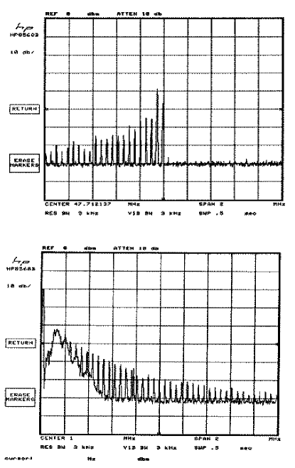
Figure 2: Three-wave coupling spectrum for longitudinal modes in a coasting beam in the Tevatron, 150 GeV beam. Excitation at h = 1000, (47.712 MHz) as shown in the upper graph, led to successive excitation of lower sidebands accompanied by low frequency modes, shown in the lower graph, which satisfy the selection rule. The lower graph begins at zero frequency and in each figure the frequency span is 2 MHz. The vertical amplitudes are in arbitrary units but the scales are logrithmic.

An interesting issue to investigate is how the power in the excited modes varies in time, especially in the presence of damping. Experimental observations indicate that a very regular cascade toward lower frequencies takes place, evidently due to successive three-wave coupling events. This behavior is typical for a dissipative system with sufficiently high mode density, and may be described by the following system of equations for the mode amplitudes.

$$\frac{\partial A_{m}}{\partial t}=s_{m}e^{i\phi}V_{mnk}A_{n}A_{k}$$ (5)

where the matrix element of the interaction has been symbolized as $V_{mnk}$, and is defined by as the following,

$$V_{mnk}=$$ (6)

$$\!\!\!\!\!\!\!\!\!\!\!\!\frac{-i\frac{2(e\omega_{s})^{3}}{\sqrt{\epsilon_{0}}(2\pi)^{2}}Z\int_{-\infty}^{\infty}\frac{\partial}{\partial\varepsilon}\!\left(\frac{\frac{\partial f_{0}}{\partial\varepsilon}}{\omega_{k}-(k)\omega(\varepsilon)}\right)\frac{1}{[\omega_{m}-m\omega(\varepsilon)]}\,d\varepsilon}{\left[\left|\frac{\partial D_{m}}{\partial\omega_{m}}\right|\left|\frac{\partial D_{n}}{\partial\omega_{n}}\right|\left|\frac{\partial D_{k}}{\partial\omega_{k}}\right|\right]^{\frac{1}{2}}}$$

It is worthwhile to note that as the multiplicity of modes becomes sufficiently dense, the coupling between waves governed by Eq. 6 can lead to a solitary wave phenomenon [11], and this subject will be described further in a later section. In the above mentioned work, only the interaction of longitudinal modes has been considered. It is also reasonable to expect that transverse modes can be coupled, especially where nonlinearities can play an important role, such as in the beam-beam interaction. This should be a fruitful area for further study.

2.3 Nonlinear Landau Damping

Sufficiently large wakefields disturb an initially smooth particle distribution by trapping particles within the potential wells of the waves generated. The particle motion decoheres with a time constant that is significantly longer than the inverse frequency spread, or linear Landau damping time. The trapped particles undergo synchrotron oscillations in the self-generated potential wells, alternately exchanging incremental energy with the wakefields. The combination of energy dispersion of the particles and the nonlinearity of the voltage waveform eventually causes phase mixing of the coherent motion. This nonlinear damping process is called nonlinear Landau damping, and was first studied in plasma physics. [6], [12] - [16].

Figure 3: Power versus time at h = 105 in response to a 0.5 msec drive pulse. The placement and duration of the drive pulse has been drawn in for reference. An impulse excitation leads to slowly decaying amplitude oscillations as trapped particles exchange energy with the wakefield.

Experiments were carried out in the Fermilab Main Ring which clearly showed the signature of nonlinear Landau damping. In these studies, a short pulse of rf power was applied to the beam using an rf cavity at h=106 (5.03 MHz). The resulting response showed a characteristic response whose envelope decayed not exponentially but in an oscillatory manner, as shown in 3. This behavior is attributed to the exchange of energy between trapped particles and waves as described above. Both analytic [16], [12], [15], and numerical work [14], on nonlinear Landau damping has been carried out which descibes the behavior we have observed. This result will also be discussed further in a later section on simulations.

It has also been pointed out [16] that the advent of particle bunching is accompanied by the appearance of coherent power in higher harmonics of the fundamental frequency of the wakefield as the trapped particle bunches compress within the potential wells. Such behavior has indeed been observed in the experiments described above [8]. This compression of the bunch length is essentially wavefront steepening which is a prerequisite for the formation of solitons.

2.4 Solitary Waves.

The formation of solitons in a beam is of interest, since solitons may well be the vehicle which carries coherent energy in a highly turbulent state that might occur in a beam with weak damping. A vast literature on solitons in various media exists [17] - [20], though little effort has been given to this subject in ultra-relativistic beams. In particular, solitons in plasmas have been studied extensively, [18], [20], which depend on the particular nonlinearity introduced by the Coulomb force, i.e. space charge. A similar space charge limit was studied for a coasting beam [21], [22], and for a resonator impedance, [23], leading to the possibility that solitons may exist in high energy beams under certain conditions.

Since a wakefield force is fundamentally more complex than the space charge force, it can be assumed that the characteristics of a soliton will also be unique to the case of a high-energy beam. In particular, it is interesting to know what the impact of the wakefield dissipation has on the solitary wave behavior. Results from a variety of beam experiments suggest that long-lived solitary structures may form and extract themselves from the core of the beam over long times [24], [25]. In other work, transient solitary waves seem to appear [8]. In all cases, solitons may be viewed as phase-space droplets that appear in the beam, and under some conditions, give rise to a phase-transition and clumpy halo formation. From this point of view, it is valuable to understand their dynamics.

To this end we sketch here the results of an analytic study of longitudinal solitons on a coasting beam due to a general resonator impedance. This reperesents the simplest possible scenario for understanding such phenomena, will illustrate the mathematical procedure and serves as the starting point for more complex situations. For the reader’s sake we note that many steps have been omitted from the following derivation for reasons of space. Full details will be given in forthcoming work [26]. The model equations for the dynamics are given by the following system

$$\frac{\partial f}{\partial T}+v\frac{\partial f}{\partial\theta}+\lambda_{1}V\frac{\partial f}{\partial v}=0,$$

$$\frac{\partial^{2}V}{\partial T^{2}}+2\gamma\frac{\partial V}{\partial T}+\omega^{2}V=\frac{\partial I}{\partial T},$$ (7)

$$I\left(\theta;T\right)=\int dvvf\left(\theta,v;T\right),$$

where $f\left(\theta,v;T\right)$ is the longitudinal distribution function, $V$ is the voltage on a resonator of $\gamma=\frac{\omega}{2Q}$, $\omega=\frac{\omega_{r}}{\omega_{s}}$ $\omega_{r}$ being the resonator frequency, and $I$ is the instantaneous beam current. Time $t$ has been normalized as $T=\omega_{s}t$. Furthermore $v=\frac{1}{\omega_{s}}\frac{d\theta}{dt}=1+\frac{k_{o}\varepsilon}{\omega_{s}}$ is the dimensionless angular velocity of a beam particle and

$$\lambda_{1}=\frac{e^{2}Rk_{o}\gamma}{\pi},$$

where $R$ is the resonator shunt impedance. Using standard moment techniques [28] on the above equations, we may pass over to the hydrodynamic picture of longitudinal beam motion and start from the system of gas-dynamic equations

$$\frac{\partial\rho}{\partial T}+\frac{\partial}{\partial\theta}\left(\rho u\right)=0,$$

$$\frac{\partial u}{\partial T}+u\frac{\partial u}{\partial\theta}=\lambda V-\frac{\sigma_{v}^{2}}{\rho}\frac{\partial\rho}{\partial\theta},$$ (8)

$$\frac{\partial^{2}V}{\partial T^{2}}+2\gamma\frac{\partial V}{\partial T}+\omega^{2}V=\frac{\partial}{\partial T}\left(\rho u\right),$$

where $\rho$ and $u$ are the density and the mean velocity moments of the distribution, respectively, (the variables $\rho$ and $V$ have been appropriately scaled) and $\lambda=\rho_{o}\lambda_{1}$. ($\rho_{o}$ = constant is the equilibrium beam density.) Using a renormalization group approach [26], [27], we may derive a set of amplitude equations for the rescaled beam density $R_{o}$, the current velocity $u_{o}$ and the mode envelope function $E$.

Before proceeding, we would like to examine the stability problem of stationary waves in this system, which can be done without a formal solution of the amplitude equations. The approach, introduced by Sagdeev [18], is to look for forms of the nonlinear equations which correspond to harmonic motion in an effective potential well. Such states, if they exist, are conjectured to be allowed solitary waves in the nonlinear system. To this end let us write down the full system of amplitude equations, which after appropriate scaling reads as

$$\frac{\partial\widetilde{\rho}}{\partial\tau}+\frac{\partial}{\partial\Theta}\left(\widetilde{\rho}\widetilde{v}\right)=0,$$

$$\frac{\partial\widetilde{v}}{\partial\tau}+\widetilde{v}\frac{\partial\widetilde{v}}{\partial\Theta}=-c_{u}^{2}\left(\frac{1}{\widetilde{\rho}}\frac{\partial\widetilde{\rho}}{\partial\Theta}+\frac{\partial\left|\psi\right|^{2}}{\partial\Theta}\right),$$ (9)

$$i\frac{\partial\psi}{\partial\tau}+i\gamma b\psi+\left(1-\widetilde{\rho}\right)\psi=-\left(1-\frac{2i\gamma}{\omega_{o}}\right)\frac{\partial^{2}\psi}{\partial\Theta^{2}}+$$

$$+\frac{2i}{\omega_{o}b}\left(1-\frac{i\gamma}{\omega_{o}}\right)\frac{\partial\left(\widetilde{\rho}\widetilde{v}\psi\right)}{\partial\Theta}+\frac{i}{\lambda b^{2}}\psi\frac{\partial\widetilde{\rho}}{\partial\tau},$$

where

$$\widetilde{\rho}=1+R_{o}\qquad;\qquad\widetilde{v}=\frac{ab\omega_{o}}{2}\left(1+u_{o}\right),$$

$$\psi=\frac{\left|\lambda\right|}{\omega_{o}\sigma_{v}}Ee^{-\gamma T}$$

are the new (rescaled) dependent variables. The coefficients entering the above expressions are specified as follows:

$$a=\frac{2}{\sqrt{\sigma_{v}^{2}+3}}\qquad;\qquad b=\frac{2\omega_{q}}{\lambda},$$

$$c_{u}=\frac{a\omega_{o}\omega_{q}\sigma_{v}}{\left|\lambda\right|},$$

where $\sigma_{v}$ is the normalized beam energy spread. The new independent variables (time $\tau$ and azimuthal position $\Theta$) are given by

$$\tau=\frac{T}{b}\qquad;\qquad\Theta=\frac{a\omega_{o}\theta}{2}.$$

Moreover in the above set of equations the following notations have been adopted

$$\omega_{o}^{2}=\omega^{2}-\lambda\qquad;\qquad\omega_{q}^{2}=\omega_{o}^{2}-\gamma^{2},$$

In order to proceed, we have to further assume that the resonator is weakly damped, namely the high-$Q$ case. For this case $\left(\gamma=0\right)$ the ansatz

$$\widetilde{\rho}=\widetilde{\rho}\left(z\right)\qquad;\qquad\widetilde{v}=\widetilde{v}\left(z\right),$$

$$\psi=A\left(z\right)e^{i\left[\left(a+v_{o}\right)z/2+\Omega\tau\right]}\quad;\quad z=\Theta-v_{o}\tau$$

leads to a system of differential equations for $\widetilde{\rho}$, $\widetilde{v}$ and $\psi$ admitting the following integrals of motion

$$C_{1}=\widetilde{\rho}\left(\widetilde{v}-v_{o}\right),$$

$$C_{2}=\frac{C_{1}^{2}}{2\widetilde{\rho}^{2}}+c_{u}^{2}\left(A^{2}+\ln\widetilde{\rho}\right),$$ (10)

$$2E=\left(\frac{dA}{dz}\right)^{2}+\left[1-\Omega+\frac{1}{4}\left(a+v_{o}\right)^{2}\right]A^{2}-$$

$$-1+\widetilde{\rho}+\frac{C_{1}^{2}}{c_{u}^{2}\widetilde{\rho}}.$$

These integrals of motion suggest that the stability of stationary waves can be equivalently described in terms of motion of a single particle in a (pseudo)- potential well. Indeed, the function

$$U\left(A\right)=\left[1-\Omega+\frac{1}{4}\left(a+v_{o}\right)^{2}\right]A^{2}-$$

$$-1+\widetilde{\rho}+\frac{C_{1}^{2}}{c_{u}^{2}\widetilde{\rho}}$$ (11)

provided $\widetilde{\rho}$ is expressed in terms of $A$ from the second integral, comprises a pseudo-potential function. In Fig. 4 we show $U\left(A\right)$ for the simplest case of constant current velocity $\widetilde{v}=v_{o}$ $\left(C_{1}=0\right)$. We note that a minimum in this pseudo-potential corresponds to solitary waves that can be effectively “trapped” in this potential well.

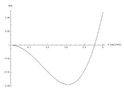
Figure 4: Pseudo-potential based on the nonlinear wave equations for a coasting beam. A minimum in this potential indicates the possibility for solitary waves (cavitons) to form.

In the following, we can proceed to find approximate closed-form solutions of these nonlinear equations, which will allow us to explicitly find the time behavior of the solitary waves in the presence of dissipation. Eliminating of the current velocity from the complete set of amplitude equations and expressing $\widetilde{\rho}$ in terms of $\left|\psi\right|^{2}$

$$\widetilde{\rho}=1-\left|\psi\right|^{2}$$ (12)

we finally arrive at the damped nonlinear Schrödinger equation

$$i\frac{\partial\psi}{\partial\tau}+i\gamma b\psi=$$

$$-\left(1-\frac{2i\gamma}{\omega_{o}}\right)\frac{\partial^{2}\psi}{\partial x^{2}}+\frac{a\gamma}{\omega_{o}}\frac{\partial\psi}{\partial x}-\left|\psi\right|^{2}\psi,$$ (13)

where

$$x=\frac{a}{2}\left(\omega_{o}\theta+\frac{2T}{b}\right).$$

Eq. 13 admits closed form solutions that indicate solitary waves can exist, but due to the dissipation in the model, eventually disappear after initial generation. We interpret this behavior as a gradual shrinking of the potential well that occurs when the trapped particles have decelerated sufficiently from the the resonantor frequency. The results for the voltage amplitude and soliton (caviton) density are shown in Figs. 5 and 6 respectively. We note that a similar equation has been derived [22] from an entirely different perspective. It is also worth noting that Eq. 13 is a special case of the complex, cubic Ginzburg-Landau equation [29], widely used to study various pattern formation phenomena and coherent structures.

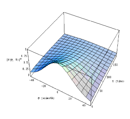
Figure 5: Voltage amplitude evolution of the solitary wave due to a resonator impedance. In the frame of the wave, the amplitude persists for long times but eventually damps as the soliton decelerates away from the beam core, and hence, the resonator’s resonant frequency.

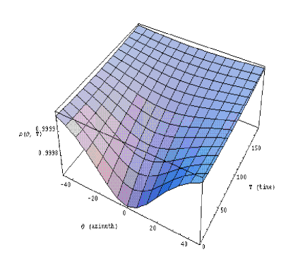
Figure 6: Caviton density evolution. A density depression associated with the solitary wave decreases in amlitude at long times as the wave amplitude itself decreases.

2.5 Turbulence.

The study of turbulence in beams is valuable primarily because it may be a universal phenomenon, at least at low levels, which plays a role in determining the limiting phase-space density in any machine. The effect has likely been small in machines well below their stability thresholds, however, as intensities have been pushed closer to stability limits, nonlinear wave interactions can occur which lead to a marginally stable equilibrium. A first attempt at determining the fluctuation spectrum for a beam was obtained by considering the equilibrium state of a Gaussian beam [30]. The resulting spectrum was related to the linear dielectric function and showed that the fluctuation density would be strongly peaked for cases near the linear stability limit. It is our conjecture that such a situation may have occurred in the Fermilab Tevatron during recent attempts to realize stochastic cooling of bunched beams [31]. A broad, stationary spectrum of fluctuations was observed at many times the expected Schottky, or shot noise, levels. The harmonic generation observed in the Fermilab Main Ring mentioned above is consistent with these observations as well. It is our aim in this paper to outline a theoretical approach to understand the formation of an equilibrium spectrum and to understand the spectral amplitude dependence on the character of the machine impedance.

The approach taken is to develop a statistical description of fluctuations for an ensemble of coupled modes. This may be viewed as a development of the amplitude equations associated with coupled modes, as in Eq. 6. The interaction between modes may be three-wave, as given in 6, or higher-order. In this work, we outline a general procedure, but keep only interactions up to the three-wave level. The result will be a scaling law for the envelope of the fluctuation spectrum.

The starting point for our analysis is the system of equations for the fluctuation $\delta N$ of the microscopic phase space density and the fluctuation $\delta V$ of the voltage [9]

$$\left(\frac{\partial}{\partial\theta}+v\frac{\partial}{\partial\sigma}+\lambda V\frac{\partial}{\partial v}\right)\delta N=$$

$$-\lambda n\frac{\partial f}{\partial v}\delta V-\lambda\frac{\partial}{\partial v}\left[\delta N\delta V-\left\langle\delta N\delta V\right\rangle\right],$$

$$\frac{\partial^{2}\delta V}{\partial\sigma^{2}}-2\gamma\frac{\partial\delta V}{\partial\sigma}+\omega^{2}\delta V=-\frac{\partial\delta I}{\partial\sigma},$$

$$\delta I=\int dv\left(1+v\right)\delta N\left(\sigma,v;\theta\right)$$

written in the variables $\sigma=\theta-\omega_{s}t$ and $v=k_{o}\varepsilon/\omega_{s}$. Fourier transforming the above equations and using the concept of slowly varying amplitude of weakly nonlinear waves one obtains the following equation

$$\left(\frac{\partial}{\partial\theta}+\Omega_{g}\frac{\partial}{\partial\sigma}-\Gamma_{k}\right)\delta V_{k}=-\frac{i}{\left(\frac{\partial\epsilon}{\partial\Omega}\right)_{\Omega_{k}}}$$

$$\times\sum_{k_{1}+k_{2}=k}\kappa_{2}\left(k,\Omega_{k_{1}}+\Omega_{k_{2}};k_{2},\Omega_{k_{2}}\right)$$

$$\times\left(\delta V_{k_{1}}\delta V_{k_{2}}-\left\langle\delta V_{k_{1}}\delta V_{k_{2}}\right\rangle\right)e^{i\theta\left(\Omega_{k}-\Omega_{k_{1}}-\Omega_{k_{2}}\right)}+...$$ (14)

for the amplitudes $\delta V_{k}$, where

$$\epsilon\left(k,\Omega\right)=1+i\lambda nZ\left(k\right)\int\frac{dv\left(1+v\right)}{\Omega-kv+io}\frac{\partial f}{\partial v},$$

is the dielectric permittivity and

$$\kappa_{2}\left(k,\Omega;k_{1},\Omega_{1}\right)=\frac{n\lambda^{2}Z\left(k\right)}{2\gamma}\int dv\left(1+v\right)$$

$$\times\frac{1}{\Omega-kv+io}\frac{\partial}{\partial v}\left(\frac{1}{\Omega_{1}-k_{1}v+io}\frac{\partial f}{\partial v}\right)$$

is the second order susceptibility of the beam. Here

$$Z\left(k\right)=\frac{ik}{k^{2}-\omega^{2}+2i\gamma k}$$

is the familiar resonator impedance function and

$$\Omega_{g}=-\left\{\frac{\partial Re\left[\epsilon\left(k,\Omega\right)\right]}{\partial k}\left[\frac{\partial Re\left[\epsilon\left(k,\Omega\right)\right]}{\partial\Omega}\right]^{-1}\right\}_{\Omega=\Omega_{k}}$$

$$\Gamma_{k}=\left\{Im\left[\epsilon\left(k,\Omega\right)\right]\left[\frac{\partial Re\left[\epsilon\left(k,\Omega\right)\right]}{\partial\Omega}\right]^{-1}\right\}_{\Omega=\Omega_{k}}$$

are the group velocity of waves and the damping factor respectively. For the slowly evolving part $A_{k}$ of the wave amplitude $\delta V_{k}$ it is straightforward to derive the equation

$$\left(\frac{\partial}{\partial\theta}+\Omega_{g}\frac{\partial}{\partial\sigma}+i\omega_{k}-\Gamma_{k}\right)A_{k}=$$

$$=i\sum_{k+k_{1}=k_{2}+k_{3}}S\left(k,k_{1},k_{2},k_{3}\right)$$

$$\times\left(A_{k_{1}}^{*}A_{k_{2}}A_{k_{3}}-A_{k_{2}}\left\langle A_{k_{1}}^{*}A_{k_{3}}\right\rangle-\left\langle A_{k_{1}}^{*}A_{k_{2}}A_{k_{3}}\right\rangle\right),$$ (15)

where

$$S\left(k,k_{1},k_{2},k_{3}\right)=\frac{\kappa_{2}\left(k-k_{2},\Omega_{k_{3}}-\Omega_{k_{1}};k_{3},\Omega_{k_{3}}\right)}{\sqrt{\omega^{2}-\lambda n}\left(\frac{\partial\epsilon}{\partial\Omega}\right)_{\Omega_{k}}\left(\frac{\partial\epsilon}{\partial\Omega}\right)_{\Omega_{k-k_{2}}}}$$

$$\times[\kappa_{2}(k,\Omega_{k_{2}}+\Omega_{k-k_{2}};k-k_{2},\Omega_{k-k_{2}})$$

$$+\kappa_{2}(k-k_{2},\Omega_{k_{2}}+\Omega_{k-k_{2}};k_{2},\Omega_{k_{2}})],$$

$$\omega_{k}=\Omega_{k}-sign\left(k\right)\sqrt{\omega^{2}-\lambda n}.$$

Averaging of the equation for $A_{k}$ yields the kinetic equation for waves

$$\left(\frac{\partial}{\partial\theta}+\Omega_{g}\frac{\partial}{\partial\sigma}-2\Gamma_{k}\right)I_{k}=$$

$$=2\pi\sum_{k+k_{1}=k_{2}+k_{3}}\left|S\left(k,k_{1},k_{2},k_{3}\right)\right|^{2}$$

$$\times\delta\left(\omega_{k}+\omega_{k_{1}}-\omega_{k_{2}}-\omega_{k_{3}}\right)$$

$$\times\left(I_{k_{1}}I_{k_{2}}I_{k_{3}}+I_{k}I_{k_{2}}I_{k_{3}}-I_{k}I_{k_{1}}I_{k_{3}}-I_{k}I_{k_{1}}I_{k_{2}}\right),$$ (16)

where

$$\left\langle A_{k}A_{k_{1}}\right\rangle=I_{k}\delta\left(k+k_{1}\right).$$

Dimensional analysis of the kinetic equation for waves gives the following fluctuation spectrum law of Kolmogorov type

$$I_{k}\sim const*k^{-7/3}.$$ (17)

We note that this power law spectrum, which in this case is due to a resonator, would indeed lead to the type of broad fluctuation spectrum seen in experiments. However, at this time, a detailed study of the scaling of the observed spectrum has not been made. An extension of the above work to consider bunched beams, and other types of machine impedance would be very worthwhile.

3 Simulations

In this work, we are interested in demonstrating examples of the nonlinear wave behavior we have described analytically. No attempt is made to closely model a real device, though this could be done with the building blocks we provide here. We shall concentrate on the longitudinal plane, as explained above, and carry out simulations exculsively on a coasting, (unbunched) beam, for simplicity. We adopt the resonator model described above and follow approximately the procedure adopted in early simulation work [32]. The particle evolution equations are given by

$$\frac{d\epsilon}{dt}=2\pi e\omega_{s}V(t)$$

$$\frac{d\theta}{dt}=-\eta\epsilon$$

$$\frac{dV}{dt}=\frac{\omega_{r}R}{Q}(I-I_{1})-\frac{\omega_{r}}{Q}V$$ (18)

$$\frac{dI_{1}}{dt}=\frac{\omega_{r}Q}{R}V$$

where $\epsilon$ is the energy deviation from the synchronous energy and V is the voltage induced in a resonator with shunt impedance R, resonant frequency $\omega_{r}$ and quality factor Q. I is the instantaneous current given as the projection of phase-space onto the $\theta$ axis

$$I=\frac{e\omega_{s}}{2\pi}\int_{-\infty}^{\infty}fd\epsilon$$

The energy dispersion $\eta$ is assumed to be a constant and the particle distribution is advanced each time step according to Eq. 18. Then the current is computed, followed by the voltage on the resonator using Eq. 18. Results for the case of a coasting beam are shown in Figure 7 - 9. The simulation parameters are given in Table 1.

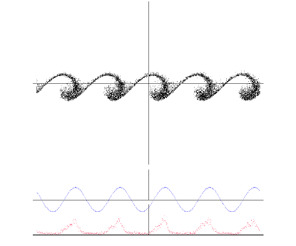
Figure 7: Simulation after 500 time steps for the model problem listed in Table 1. The upper portion represents $\varepsilon-\theta$ phase-space. The middle curve is the cavity voltage as applied to different portions of the beam and the bottom curve is the projection of phase-space on the theta-axis, representing the instantaneous current. The resonator wakefields have caused bunching which shows significant particle trapping and consequent wave overturning. The particle current shows strong local intensification of the beam density corresponding to the solitons.

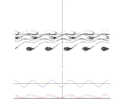
Figure 8: Phase-space after 1000 time steps. Portions of the originally trapped particle population have decelerated from the core due to the finite resistivity of the wakefields. The solitons remain, however, well-organized as they experience deceleration. Both the cavity voltage and the density perturbations have decreased, but persist for long times. The diagrams have the same meaning as in the previous figure.

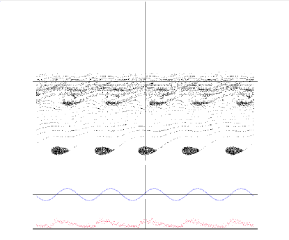
Figure 9: Phase-space after 2000 time steps. The beam core is now largely decohered, however, the solitons continue to decelerate slowly and maintain the remaining cavity voltage well off resonance. The diagrams have the same meaning as in the previous figure.

In Fig. 7, the phase-space distribution is shown, initially assumed to be uniform in $\theta$ and Gaussian in energy. After 500 time steps, the resonator has developed a sinusoidal voltage from the initial noise level (due to the finite number of particles) which has succeeded in bunching a large fraction of the beam and synchrotron motion in the resulting potential well is taking place. The synchrotron motion can also be thought of as synonymous to the wave-breaking process which has been described in plasma physics [12]. As time proceeds, Fig. 8, shows a deceleration of the trapped particles from the core of the beam, and the decelerated portion remains well-organized, and even intensifies as its length is foreshortened. The voltage in the resonator then becomes phase-locked to the ’droplets’ and the voltage amplitude oscillates as they move in and out of phase with the remaining coherent structure in the beam’s core. We note that the droplets thus formed bear the characteristics of the solitons discussed in the previous section, remaining self-organized for long times.

As the dissipation in the impedance continues to decelerate the solitons Fig. 9, the resonator voltage drops due to the high Q value, or narrow bandwidth, assumed. This, in turn, reduces the deceleration rate and the depth of the potential wells that can sustain the solitons. As such, a steady state can be reached where the remaining trapped particles reach a stable equilibrium outside the beam, in accord with the analytic model for solitary waves. The envelope of the cavity voltage and the mean energy deviation of the solitons are shown in Fig. 10, indicating deceleration of the trapped particles. A steady state is eventually reached, though not shown, where the solitons have moved sufficiently off resonance that the deceleration ceases.

We show the final results for a low-Q cavity in Fig. 11. These are qualitatively the same as in the previous case, but the structure of the solitons has taken on a decidedly random character. This is evidently due to the fact that the fractional contribution of noise to the cavity voltage is larger, owing to the wider bandwidth of the cavity, resulting in a more random distribution of potential well sizes. Droplet, or soliton formation, still occurs, but the resulting fluctuation spectrum is broader. The onset of the solitary waves can be viewed as a phase transition at the beam’s edge produced by the resonator’s wakefield. This is the case, we believe, that is most frequently encountered in actual machines.

Table 1: Model Simulation Parameters

Parameter	Value
Resonator Impedance	100 Ohms
Slip Factor $\eta$	.001
Resonator Quality Factor	10.
Typical Beam Energy Spread $\sigma_{\varepsilon}/E_{0}$	$1-4\times 10^{-3}$
Number of Particles	10000

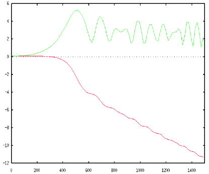
Figure 10: Cavity voltage envelope and mean energy deviation. The upper curve is the envelope of the cavity voltage, showing the exchange of energy between the soliton and the wakefield. The lower curve is the mean energy of the perturbation, which descends away from the beam, but eventually reaches an equilibrium (not shown) where the deceleration ceases.

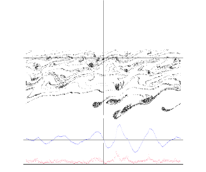
Figure 11: Simulation results for low-Q case. The comparative contribution of noise to the dynamics is larger owing to the increased bandwidth of the resonator. Solitary waves still develop, but the associated fluctuation spectrum is broader.

We note that the fluctuation spectrum associated with the above distribution is due to the ensemble of strongly nonlinear waves and is likely beyond the realm of the three-wave interaction described in the scaling law in the previous section. An interesting study to be carried out is the experimental and theoretical determination of the spectral shape in a machine whose impedance is well-known.

4 Conclusions

In this work we have attempted to outline various levels of nonlinearity in coherent interactions in high-energy beams. Besides the general academic interest of nonlinear dynamics, for which high-energy beams provide an excellent testing ground, there are at least two areas where the study of nonlinear waves can find application in accelerator physics.

The first is the study of halo formation in which the nonlinear evolution of coherent fluctuations can lead to soliton, or droplet, formation, as described in previous sections. While there is suggestive experimental evidence that such states can occur, there has been little detailed study of this phenomenon, and we assert that there is much to be learned about machine wakefields through the study of solitary waves and their interactions. Specifically, we have only considered the simplest case, that of longitudinal waves in an unbunched beam, and there are many other cases of interest in high-energy accelerators.

The second application is the study of non-equilibrium fluctuations driven by wakefields. Nonlinear mode-mode coupling permits a frequency cascade, both toward lower and higher frequencies via separate processes. The photon distribution that results is an equilibrium between the nonlinear interactions producing the cascade and weak dissipative mechanisms. These mechanisms are assumed to be related to the broadband impedance of the machine, though other mechanisms may also be responsible. We have carried out a model calculation for a specific form of impedance that yields a specific scaling law for the turbulent spectrum. A number of assumptions come into play in the development of this model and the situation is ripe for careful experimental testing. The benefit of this study is the understanding of the significance of low-level turbulence in the limiting parameters of a given accelerator.

5 Acknowledgements

The authors are indebted to Prof. Nigel Goldenfeld for helpful discussions, and to Dr. David Finley for his enlightened support of this work.

References

- [1] A. Hofmann, Single-beam Collective Phenomena - Longitudinal,CERN 77-13, July 1977.
- [2] C. F. Kennel and F. Engelmann, Velocity Space Diffusion from Weak Plasma Turbulence in a Magnetic Field, Physics of Fluids, 9, 1966.
- [3] Y. Chin and K. Yokoya, Physical Review D, Vol. 28, 1983
- [4] A. Bogacz and K. Y. Ng, Nonlinear Saturation of the Longitudinal Modes of a Coasting Beam in a Storage Ring, Physical Review D, D36, 1987
- [5] A. Gerasimov, Longitudinal Bunched-Beam Instabilities Going Nonlinear: Emittance Growth, Beam Splitting and Turbulence, Physical Review E, Vol. 49, 1994
- [6] T.M. O’Neil, Collisionless Damping of Nonlinear Plasma Oscillations, The Physics of Fluids, Vol. 8, Dec 1965.
- [7] K. Nishikawa, Parametric Excitation of Coupled Waves I.General formulation, Journal of the Physical Society of Japan, Vol. 24, 1968.
- [8] L. K. Spentzouris, Ph.D. Thesis, Northwestern University, 1996.
- [9] V. E. Zakharov, Kolmogorov Spectra in Weak Turbulence Problems, Handbook of Plasma Physics, Eds. M. N. Rosenbluth and R. Z. Sagdeev, Elsevier, 1984.
- [10] T. H.. Stix, The Theory of Plasma Waves, American Institute of Physics, New York, 1992.
- [11] E. Fermi, J. Pasta and S. Ulam, Studies of Nonlinear Problems, Los Alamos National Laboratory Report LA-1940, 1955.
- [12] J. Dawson, On Landau Damping, The Physics of Fluids, Vol. 4, Number 7, Jul 1961.
- [13] J. H. Malmberg and C. B.Wharton, Physical Review Letters, Vol. 17, 175, 1966.
- [14] I.H. Oei and D.G. Swanson, Self-consistent Finite Amplitude Wave Damping, The Physics of Fluids, Vol. 15, Number 12, Dec 1972.
- [15] J. Canosa and J. Gazdag, Threshold Conditions for Electron Trapping by Nonlinear Waves, The Physics of Fluids, Vol. 17, Number 11, Nov 1974.
- [16] T.M. O’Neil, J.H. Winfrey, and J.H.Malmberg, Nonlinear Interaction of a Small Cold Beam and a Plasma, The Physics of Fluids, Vol 14, Number 6, June 1971.
- [17] P. G. Drazin and R. S.Johnson, Solitons: An Introduction, Cambridge University Press, Cambridge, 1989.
- [18] R. Z. Sagdeev, D. A. Usikov and G. M. Zaslavsky, Nonlinear Physics, Harwood Academic, London, 1988
- [19] A.C. Scott, F.Y.F. Chu, and D.W. McLaughlin, The Soliton: a New Concept in Applied Science, Proceedings of the IEEE, Vol 61, Number 10, Oct 1973.
- [20] R. C. Davidson, Methods in Nonlinear Plasma Theory, Academic Press, New York, 1972.
- [21] J.J. Bisognano, Solitons and particle beams, Particles and fields series 47, High Brightness Beams for Advanced Accelerator Applications, AIP Conference Proceedings 253, College Park MD, 1991.
- [22] R. Fedele, G. Miele, L. Palumbo, and V. G. Vaccaro, Thermal Wave Model for Nonlinear Longitudinal Dynamics in Particle Accelerators, Physics Letters, A 179, 407, 1993.
- [23] P. L. Colestock, S. Assadi and L. K.Spentzouris, Nonlinear Collective Phenomena in High-Energy Synchrotrons, Proc. ICFA Workshop on Nonlinear and Collective Phenomena in Beam Physics, AIP Proc. 395, Arcidosso, 1996.
- [24] M. Q. Barton and C. E. Nielsen, Longitudinal Instability and Cluster Formation in the Cosmotron, Proc. Int. Conf. on High-Energy Accelerators, Sept. 6-12, 163, 1961.
- [25] R. A. Carrigan, Private Communication
- [26] S. Tzenov and P. L. Colestock, To Be Published
- [27] L.-Y. Chen, N. .Goldenfeld and Y.Oono, Renormalization Group and Singular Perturbation: Multiple Scales, Boundary Layers and Reductive Perturbation Theory, Phys. Rev E, Vol. 54, 376, 1996.
- [28] Y. L. Klimontovich, Statistical Physics, Harwood Academic Publishers, Chur. 1986.
- [29] M. C.Cross and P. C.Hohenberg, Pattern Formation Outside of Equilibrium, Reviews of Modern Physics, Vol. 65, 851, 1993.
- [30] V. V. Parkhomchuk and D. V. Pestrikov, Thermal Noise in an Intense Beam in a Storage Ring, Sov. Phys. Tech. Phys., Vol. 25, 7, 1980.
- [31] G. P. Jackson, Bunched Beam Stochastic Cooling in the Fermilab Tevatron Collider, Proc. Montreaux Workshop on Beam Cooling and Related Topics, CERN Geneva, CERN-94-03, 127, 1993.
- [32] E. Keil and E. Messerschmid, Study of Non-Linear Effects of a Resonant Cavity on the Longitudinal Dynamics of a Coasting Particle Beam, Nucl. Inst. and Methods, Vol. 128, 203, 1975.