Towards an understanding of lineage specification in hematopoietic stem cells:
A mathematical model for the interaction of transcription factors GATA-1 and PU.1

Abstract

In addition to their self-renewal capabilities, hematopoietic stem cells guarantee the continuous supply of fully differentiated, functional cells of various types in the peripheral blood. The process which controls differentiation into the different lineages of the hematopoietic system (erythroid, myeloid, lymphoid) is referred to as lineage specification. It requires a potentially multi-step decision sequence which determines the fate of the cells and their successors. It is generally accepted that lineage specification is regulated by a complex system of interacting transcription factors. However, the underlying principles controlling this regulation are currently unknown.

Here, we propose a simple quantitative model describing the interaction of two transcription factors. This model is motivated by experimental observations on the transcription factors GATA-1 and PU.1, both known to act as key regulators and potential antagonists in the erythroid vs. myeloid differentiation processes of hematopoietic progenitor cells. We demonstrate the ability of the model to account for the observed switching behavior of a transition from a state of low expression of both factors (undifferentiated state) to the dominance of one factor (differentiated state). Depending on the parameter choice, the model predicts two different possibilities to explain the experimentally suggested, stem cell characterizing priming state of low level co-expression. Whereas increasing transcription rates are sufficient to induce differentiation in one scenario, an additional system perturbation (by stochastic fluctuations or directed impulses) of transcription factor levels is required in the other case.

1 Introduction

The hematopoietic system consists of a variety of functionally different cell types, including mature cells such as erythrocytes, granulocytes, platelets, or lymphocytes, as well as several different precursor cells (i.e., premature cell stages) and hematopoietic stem cells (HSC) (Lord, 1997; Orkin, 2000). Most mature cell types have limited life spans ranging from a few hours to several months, which implies the existence of a source capable of replenishing these differentiated cells throughout the life span of an individual. This supply is realized by the population of HSC, which is maintained and even regenerated after injury or depletion throughout the whole life of the organism. This self-renewal property is a major characteristic defining HSC (Loeffler and Roeder, 2002; Lord, 1997; Potten and Loeffler, 1990). A second major characteristic of HSC is their ability to contribute to the production of cells of all hematopoietic lineages, thus ensuring the supply of functionally differentiated cells meeting the needs of the organism. The process controlling the development of undifferentiated stem or progenitor cells into one specific functional direction (i.e., one specific hematopoietic lineage) is called lineage specification. It is generally accepted that the process of lineage specification is governed by the interplay of many different transcription factors (Akashi, 2005; Cantor and Orkin, 2002; Cross et al., 1994; Orkin, 1995, 2000; Tenen, 2003). Experimental results suggest that a number of relevant transcription factors are expressed simultaneously in HSC, although at a low level (Akashi et al., 2003; Hu et al., 1997). Some authors refer to this state of a low level co-expression as priming behavior (Akashi, 2005; Cross and Enver, 1997; Enver and Greaves, 1998). During differentiation the balanced co-expression of these potentially antagonistic transcription factors is assumed to be broken at some point (or even multiple points). Thereafter, the system is supposed to be characterized by an up-regulated level of some transcription factors, specific for a particular lineage, while other transcription factors are down-regulated. These observations suggest a transcription factor network, capable of switch-like behavior by changing from unspecific co-expression to different states of specific expression. However, the general underlying principles of the regulatory mechanisms are currently unknown. Particularly, it is unclear whether the assumption of a dynamically balanced low level co-expression state is justified or whether priming should rather be interpreted as the result of an inactive transcription factor network overlaid by stochastic fluctuations of transcription factor expression.

In this paper we propose a simple mathematical model describing different interaction scenarios of two transcription factors. Biologically, this simple two component network model is motivated by experimental observations on the transcription factors GATA-1 and PU.1, known to be involved in the process of lineage specification of HSC (Du et al., 2002; Oikawa et al., 1999; Rekhtman et al., 1999; Rosmarin et al., 2005; Tenen, 2003; Voso et al., 1994). The zinc finger factor GATA-1 is reported to be required for the differentiation and maturation of erythroid/megakaryocytic cells, while the Ets-family transcription factor PU.1 supports the development of myeloid and lymphoid cells (reviewed by Cantor and Orkin, 2002; Tenen, 2003). For both, GATA-1 and PU.1, it has been demonstrated that they are able to stimulate their own transcription through an auto-catalytic process (Chen et al., 1995; Nishimura et al., 2000; Okuno et al., 2005; Tsai et al., 1991). Additionally, there are physical interactions between GATA-1 and PU.1 which induce a mutual inhibition and, therefore, favor one lineage choice at the expense of the other (erythroid/megakaryocyte vs. myeloid) (Du et al., 2002; Nerlov et al., 2000; Rekhtman et al., 1999, 2003; Voso et al., 1994; Yamada et al., 1998; Zhang et al., 1999, 2000). In particular, two different mechanisms for the mutual inhibition of these two transcription factors have been suggested by experimental observations: On one hand, GATA-1 binds to the $\beta 3/\beta 4$ region of PU.1 (complex 1) and displaces the PU.1 co-activator c-Jun from its binding site, thereby, inhibiting the transcription initiation of PU.1 (Zhang et al., 1999). On the other hand, the inhibition of GATA-1 transcription is mediated by the binding of the N-terminal region of PU.1 to the C-finger region of GATA-1 (complex 2), thus blocking the binding of GATA-1 to its promoter (Zhang et al., 2000). That means, although both inhibition mechanisms are interfered through the formation of PU.1/GATA-1 heterodimers, the two complexes are structurally different. Whereas complex 1 (inhibition of PU.1 transcription by GATA-1) is known to bind to DNA, thus occupying a PU.1 promoter site, DNA-binding of complex 2 (inhibition of GATA-1 transcription by PU.1) has not been reported so far.

The mechanisms of antagonistic interdependence together with positive auto-catalytic regulation provide a framework for the theoretical investigation of different scenarios of transcription factor interaction and their implications for the explanation of lineage specification control. Applying a mathematical model, which formalizes the described interactions, it is now possible to analyze different combinations of transcription factor activation and inhibition on a qualitative and quantitative level. The proposed model relies on principles suggested for the description of general genetic switches (e.g. Becskei et al., 2001; Cinquin and Demongeot, 2002, 2005; Gardner et al., 2000).

In this paper it is our objective to examine the following questions within the framework of this model structure:

• Are the experimentally described interactions of the two transcription factors sufficient to generate a switching behavior between a stable co-expression of two factors and the dominance of one of these factors?

• What are the conditions inducing such a qualitative change in the system behavior?

• Is there evidence for a functional role of the (experimentally suggested) priming status?

To answer these question the following strategy is applied. Firstly, the model equations are derived on the basis of the described biological mechanisms of transcription factor interaction for GATA-1 and PU.1 (Section 2). Secondly, this model is analyzed with respect to the existence of steady state solutions and their dependence on the model parameters. According to our objective, to understand the mechanisms leading to switches between different stable system states, we focus our analysis particularly on the determination of bifurcation conditions, considering different scenarios of transcription factor interaction (Section 3). Finally, the obtained results are discussed in relation to the ongoing debate about lineage specification control in the hematopoietic system, specifically with respect to potential explanations of the experimentally suggested low level co-expression of transcription factors (priming) in undifferentiated progenitors and stem cells (Section 4).

2 Model description

Although our analysis is motivated by experimental observations of specific transcription factor interactions (GATA-1 and PU.1), the model may also be applied in the general context of two interacting transcription factors. In the following, the two transcription factors are denoted by $X$ and $Y$.

2.1 General assumptions

The general design of the model structure is based on the following assumptions which are motivated by the experimental observations outlined in Section 1:

• Both transcription factors, $X$ and $Y$, are able to act as activator molecules:

  • If bound to their own promoter region, $X$ and $Y$ introduce a positive feedback on their own transcription. This process is referred to as specific transcription (Fig. 1(a)).

  • $X$ and $Y$ are both able to induce an overall transcription which also effects potentially antagonistic transcription factors. Although such an interaction is most likely indirect, for the model we consider a mutual activation of $X$ and $Y$ by the opposing transcription factor, which we refer to as unspecific transcription (Fig. 1(b)).

  We assume that transcription initiation is only achieved by the simultaneous binding of two $X$ and $Y$ molecules, respectively (i.e., binding cooperativity $c=2$). This assumption is motivated by the result that a binding cooperativity $c>1$ is a necessary condition for the existence of system bistability (see e.g. Becskei et al., 2001; Cinquin and Demongeot, 2005; Gardner et al., 2000).

• There is a mutual inhibition of $X$ and $Y$. Within this context, two possible mechanisms, based on the formation of two structurally different complexes of $X$ and $Y$, are considered:

  • Joint binding of $X$ and $Y$ molecules to promoter sites (Fig. 1(c)). Here, the DNA-bound $XY$-complex ($Z_{1}$) acts as a transcription repressor, which blocks the binding sites. This represents a mode of competition for free binding sites.

  • Formation of another $XY$-complex, called $Z_{2}$, which neither binds to $X$ nor $Y$ DNA binding site (Fig. 1(d)). In contrast to $Z_{1}$, this represents a competition for free transcription factor molecules.

  Both inhibition mechanisms (including combinations of them) are considered for $X$ as well as for $Y$.

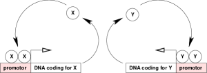
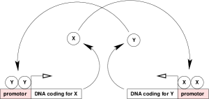
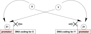
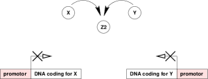
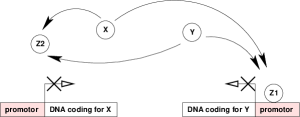
Figure 1: Principles of transcription initiation and inhibition for $X$ and $Y$. (a) Specific transcription, i.e. auto-catalysis by the transcription factor itself; (b) Unspecific transcription, i.e. transcription initiated by another transcription factor; (c-e) Suggested mechanisms of transcription inhibition for $X$ and $Y$ by formation of $XY$-complexes: (c) A $XY$-complex, called $Z_{1}$, bound to the promoter regions acts as a repressor; (d) The formation of a structurally different $XY$-complex ($Z_{2}$) competitively inhibits the DNA binding of $X$ and $Y$ molecules; (e) Combination of (c) and (d) as suggested for GATA-1 and PU.1 (Zhang et al., 1999, 2000)

To facilitate the analysis of the mathematical model we make the following simplifications:

• Post-transcriptional regulation is neglected, i.e., the transcription of a gene is considered to ultimately result in the production of the corresponding protein (here, a transcription factor).

• Time delays due to transcription and translation processes are neglected.

• Simultaneous binding of $X$/$Y$ monomers together with a $Z_{1}$-heterodimer, of two $Z_{1}$-heterodimers, as well as of a $X$ and a $Y$ monomer at the same promoter are excluded from the analysis.

• Interactions of $X$, $Y$ as well as the promoter regions of the coding genes with further transcription factors are neglected.

Throughout the paper the following notations are used: $x,y$ denote the molecule concentrations of $X$ and $Y$, respectively. $Z_{1}$ denotes the DNA bound $XY$-complex and $Z_{2}$ the structurally different $XY$- complex, which is not able to bind to promoter DNA. $D_{x/y}$ denotes free DNA binding sites within the promoter region of $X$ and $Y$, respectively. In contrast, binding sites occupied by $X$ or $Y$ molecules or by the $XY$-complex $Z_{1}$ are denoted as $D_{x/y}^{xx/yy/xy}$.

2.2 Model equations

With these assumptions one can write down a set of chemical reaction equations which underly the system dynamics.

The processes of specific and unspecific transcription activation (see Fig. 1(a),(b)) are described by equations (1)-(4).

$$X+X+D_{x}\stackrel{{\scriptstyle K_{1}}}{{\rightleftharpoons}}D_{x}^{xx} ;\quad D_{x}^{xx}\stackrel{{\scriptstyle s_{x}}}{{\rightarrow}}D_{x}^{xx}+X$$ (1)

$$Y+Y+D_{x}\stackrel{{\scriptstyle K_{2}}}{{\rightleftharpoons}}D_{x}^{yy} ;\quad D_{x}^{yy}\stackrel{{\scriptstyle u_{x}}}{{\rightarrow}}D_{x}^{yy}+X$$ (2)

$$Y+Y+D_{y}\stackrel{{\scriptstyle K_{3}}}{{\rightleftharpoons}}D_{y}^{yy} ;\quad D_{y}^{yy}\stackrel{{\scriptstyle s_{y}}}{{\rightarrow}}D_{y}^{yy}+Y$$ (3)

$$X+X+D_{y}\stackrel{{\scriptstyle K_{4}}}{{\rightleftharpoons}}D_{y}^{xx} ;\quad D_{y}^{xx}\stackrel{{\scriptstyle u_{y}}}{{\rightarrow}}D_{y}^{xx}+Y$$ (4)

Herein we made the simplifying assumption that the DNA binding of $X$ and $Y$ always occurs as the binding of homodimers. That means, that the sequential binding of two monomers, as the second possibility of DNA binding, is not consider. The process of dimerization, as well as the DNA binding and dissociation, are regarded to be in quasi steady state.

Here and throughout the paper, the $K_{i}={k_{i}}/{\bar{k}_{i}}\;(i=1,...,7)$ denote the equilibrium (dissociation) constants of the reactions, with $k_{i}$ and $\bar{k}_{i}$ representing the forward and backward reaction rate constants, respectively. Finally, it is assumed that both transcription factor monomers, $X$ and $Y$, decay with first order kinetics at rates $k_{0}^{x}$ and $k_{0}^{y}$, whereas dimer-complexes are assumed to be stable.

The different mutual transcription inhibition mechanisms are illustrated in Figs. 1(c)-(e). First, we consider the formation the $XY$-complex $Z_{2}$ (see Fig. 1(d))

$$X+Y\stackrel{{\scriptstyle K_{5}}}{{\rightleftharpoons}}Z_{2}\,.$$ (5)

Under the quasi steady state assumption $Z_{2}$ does not contribute to the mathematical description of the system dynamics.

As shown in Fig. 1(c), there is also the possibility that $X$ and $Y$ form a structurally different heterodimer $Z_{1}$, which is able to bind to the promoter regions, acting as a repressor for $X$ and $Y$ transcription, respectively:

$$X+Y+D_{x} \stackrel{{\scriptstyle K_{6}}}{{\rightleftharpoons}}D_{x}^{xy},$$ (6)

$$X+Y+D_{y} \stackrel{{\scriptstyle K_{7}}}{{\rightleftharpoons}}D_{y}^{xy}.$$ (7)

As with the promoter binding of $X$ and $Y$, we collapse dimerization, which is assumed to be in quasi steady state, and DNA binding into one process, neglecting the sequential binding of monomers.

Under the posted quasi steady state assumptions, equations (1)-(7) lead to the following set of ordinary differential equations:

$$\frac{d{x}}{d{t}} =-k_{0_{x}}x+\frac{s_{x}K_{1}x^{2}+u_{x}K_{2}y^{2}}{1+K_{1}x^{2}+K_{2}y^{2}+K_{6}xy}$$ (8)

$$\frac{d{y}}{d{t}} =-k_{0_{y}}y+\frac{s_{y}K_{3}y^{2}+u_{y}K_{4}x^{2}}{1+K_{3}y^{2}+K_{4}x^{2}+K_{7}xy}$$ (9)

Details of the derivation are given in Appendix A.

3 Results

3.1 Symmetric system

To analytically derive steady state as well as potential bifurcation conditions, we restrict ourself in this section to the special case of a completely symmetric system, i.e.: $k_{0_{x}}=k_{0_{y}}=k_{0}$, $s_{x}=s_{y}={\tilde{s}}$, $u_{x}=u_{y}={\tilde{u}}$, $K_{1}=K_{3}$, $K_{2}=K_{4}$, and $K_{6}=K_{7}$. Using these relations, together with ${\bf x}=\sqrt{K_{1}}x$, ${\bf y}=\sqrt{K_{1}}y$, $k_{u}={K_{2}}/{K_{1}}$, $k_{r}={K_{6}}/{K_{1}}$, $s={\sqrt{K_{1}}}{\tilde{s}}/{k_{0}}$, $u={\sqrt{K_{1}}}{\tilde{u}}/{k_{0}}$, and $\tau=k_{0}t$, the system (8), (9) can be written in a dimensionless form as

$$\frac{d{{\bf x}}}{d{\tau}} =-{\bf x}+\frac{s{\bf x}^{2}+uk_{u}{\bf y}^{2}}{1+{\bf x}^{2}+k_{u}{\bf y}^{2}+k_{r}{\bf x}{\bf y}},$$ (10)

$$\frac{d{{\bf y}}}{d{\tau}} =-{\bf y}+\frac{s{\bf y}^{2}+uk_{u}{\bf x}^{2}}{1+k_{u}{\bf x}^{2}+{\bf y}^{2}+k_{r}{\bf x}{\bf y}},$$ (11)

Equations (10) and (11) are a pair of coupled first order differential equations. The steady state ($\dot{\bf x}=\dot{\bf y}=0$) is defined implicitly by

$${\bf x} =\frac{s{\bf x}^{2}+uk_{u}{\bf y}^{2}}{1+{\bf x}^{2}+k_{u}{\bf y}^{2}+k_{r}{\bf x}{\bf y}},$$ (12)

$${\bf y} =\frac{s{\bf y}^{2}+uk_{u}{\bf x}^{2}}{1+k_{u}{\bf x}^{2}+{\bf y}^{2}+k_{r}{\bf x}{\bf y}}.$$ (13)

The domain of these nullclines for ${\bf x}$ and ${\bf y}$ is restricted by the choice of parameters as outlined in Appendix B. The intersections of the nullclines correspond to the fixed points $({\bf x}^{*},{\bf y}^{*})$ of the differential equations (10) and (11). Fixed points on the diagonal $({\bf x}^{*},{\bf x}^{*})$ are traced under the simplifying condition ${\bf x}={\bf y}$. In this case, equations (12) and (13) can be summarized by

$${\bf x}^{*}=\frac{{{\bf x}^{*}}^{2}(s+uk_{u})}{1+{{\bf x}^{*}}^{2}(1+k_{u}+k_{r})}\;,$$ (14)

The first (trivial) fixed point of equation (14) is ${\bf x}^{*}_{1}=0$. Having eliminated this solution, the remaining quadratic equation yields two further non-trivial fixed points at

$${\bf x}^{*}_{2/3}=\frac{(s+uk_{u})\pm\sqrt{(s+uk_{u})^{2}-4(1+k_{u}+k_{r})}}{2(1+k_{u}+k_{r})}\,.$$ (15)

$({\bf x}_{2}^{*},{\bf x}_{2}^{*})$ and $({\bf x}_{3}^{*},{\bf x}_{3}^{*})$ are real fixed points on the diagonal for

$$s\geq-uk_{u}+2\sqrt{1+k_{u}+k_{r}}\,.$$ (16)

Bifurcation points can be characterized by nullclines intersecting with equal slopes. The derivatives of equations (10) and (11) are evaluated to determine explicit conditions for bifurcation occurrence on the diagonal, considering $s$ as the bifurcation parameter. For simplicity the denominators in equations (12) and (13) are defined as $P_{x}=1+{\bf x}^{2}+k_{u}{\bf y}^{2}+k_{r}{\bf x}{\bf y}$ and $P_{y}=1+k_{u}{\bf x}^{2}+{\bf y}^{2}+k_{r}{\bf x}{\bf y}$. The partial derivative of equation (12) with respect to ${\bf y}$ leads to

$${\bf x}^{\prime}=\frac{(2s{\bf x}{\bf x}^{\prime}+2uk_{u}{\bf y})P_{x}-(s{\bf x}^{2}+uk_{u}{\bf y}^{2})P_{x}^{\prime}}{P_{x}^{2}}$$ (17)

with ${\bf x}^{\prime}={\partial{{\bf x}}}/{\partial{{\bf y}}}$ and $P_{x}^{\prime}={\partial{P_{x}}}/{\partial{{\bf y}}}={\bf x}^{\prime}(2{\bf x}+k_{r}{\bf y})+2k_{u}{\bf y}+k_{r}{\bf x}$. Solving for ${\bf x}^{\prime}$ yields

$${\bf x}^{\prime}=\frac{2uk_{u}{\bf y}P_{x}-(s{\bf x}^{2}+uk_{u}{\bf y}^{2})(2k_{u}{\bf y}+k_{r}{\bf x})}{P_{x}^{2}-2s{\bf x}P_{x}+(s{\bf x}^{2}+uk_{u}{\bf y}^{2})(2{\bf x}+k_{r}{\bf y})}\,.$$ (18)

For bifurcation points on the diagonal $({\bf x}={\bf y})$, where the denominators $P_{x}$ and $P_{y}$ simplify to $P^{*}=1+{{\bf x}^{*}}^{2}(1+k_{u}+k_{r})$, equation (18) can be rewritten as

$${\bf x}^{\prime}({P^{*}}^{2}-2s{\bf x}P^{*}+{\bf x}^{3}(s+uk_{u})(2+k_{r}))=2uk_{u}{\bf x}P^{*}-{\bf x}^{3}(s+uk_{u})(2k_{u}+k_{r})\,.$$ (19)

Inserting $P^{*}$ in the form $P^{*}={\bf x}(s+uk_{u})$ derived from equation (14) and neglecting the trivial solution the equality now reads

$${\bf x}^{\prime}(uk_{u}-s+{\bf x}(2+k_{r}))=2uk_{u}-{\bf x}(2k_{u}+k_{r})\,.$$ (20)

To find the bifurcation points on the diagonal one needs to study the two distinct cases for ${\bf x}^{\prime}=1$ and ${\bf x}^{\prime}=-1$ (see Appendix C).

Case I (${\bf x}^{\prime}=1$):

Equation (20) satisfies the condition ${\bf x}^{\prime}=1$ at

$${\bf x}_{{\bf x}^{\prime}=1}=\frac{s+uk_{u}}{2(1+k_{u}+k_{r})}$$ (21)

This only coincides with the fixed points ${\bf x}^{*}_{2/3}$ derived in equation (15) if the expression under the radical in equation (15) vanishes, i.e., ${\bf x}^{*}_{2}={\bf x}^{*}_{3}$. This is true for

$$s_{1}^{*}=-uk_{u}+2\sqrt{1+k_{u}+k_{r}}\,,$$ (22)

which corresponds to the condition defined in (16). This implies that the “birth” of the fixed points $({\bf x}_{2}^{*},{\bf x}_{2}^{*})$ and $({\bf x}_{3}^{*},{\bf x}_{3}^{*})$ coincides with the bifurcation condition ${\bf x}^{\prime}=1$. The sequence of nullclines in Fig. 2(a)-(c) illustrates this behavior for an unspecific transcription rate $u=1$. The nullclines in Fig. 2(a) do not intersect for $s<s_{1}^{*}$, i.e., there is no non-trivial fixed point along the diagonal. For $s=s_{1}^{*}$ one common fixed point at ${\bf x}^{*}_{2}(s_{1}^{*})={\bf x}^{*}_{3}(s_{1}^{*})=({s_{1}^{*}+uk_{u}})/{2(1+k_{u}+k_{r})}$ exists, which marks the bifurcation point depicted in Fig. 2(b). For $s>s_{1}^{*}$ two distinct fixed points $({\bf x}_{2}^{*},{\bf x}_{2}^{*})$ and $({\bf x}_{3}^{*},{\bf x}_{3}^{*})$ exist on the diagonal, shown in Fig. 2(c). Whereas the upper point at $({\bf x}_{2}^{*},{\bf x}_{2}^{*})$ is stable, the lower one at $({\bf x}_{3}^{*},{\bf x}_{3}^{*})$ is unstable. The nullclines change qualitatively for a further increase in the bifurcation parameter $s$ as shown in the sequence Fig. 2(d),(e).

In the case of a smaller unspecific transcription rate $u=0.4$ the corresponding bifurcation is illustrated in Fig. 3(d). The two fixed points $({\bf x}_{2}^{*},{\bf x}_{2}^{*})$ and $({\bf x}_{3}^{*},{\bf x}_{3}^{*})$ generated at the diagonal are both unstable as depicted in Fig. 3(e),(f). The qualitative differences between the scenarios for small and large unspecific transcription $u$ are more thoroughly investigated in the subsequent paragraphs.

Figure 2: Deformation of the nullclines for increasing values of the bifurcation parameter $s$. The occurrence of the first bifurcation at $s_{1}^{*}$ is depicted in (b), the second bifurcation at $s_{1}^{*}=s_{2}^{*}$ in (g). Parameters are $k_{u}=1$, $k_{r}=0$ and $u=1$. The bifurcation parameter is set to $s=1.7$ (a), $s=s_{1}^{*}=-1+2\sqrt{2}\approx 1.83$ (b), $s=1.9$ (c), $s=1.99$ (d), $s=2.01$ (e), $s=2.6$ (f), $s=s_{2}^{*}=s_{3}^{*}=3u=3$ (g), $s=3.8$ (h). Fixed points are marked as follows: trivial fixed point $(0,0)$ - $\blacksquare$, stable/unstable fixed point $({\bf x}_{2}^{*},{\bf x}_{2}^{*})$ - $\blacktriangle$/$\triangle$, unstable fixed point $({\bf x}_{3}^{*},{\bf x}_{3}^{*})$ - $\triangledown$, stable/unstable fixed points off the diagonal - $\bullet$/$\circ$, bifurcation point - $\square$.

Figure 3: Deformation of the nullclines for increasing values of the bifurcation parameter $s$ for unspecific transcription rate $u=0.4$. Parameters are $k_{u}=1$ and $k_{r}=0$. The bifurcation parameter is set to $s=1.9$ (a), $s=2.04$ (b), $s=2.1$ (c), $s=s_{1}^{*}\approx 2.43$ (d), $s=2.8$ (e), $s=3.2$ (f). Fixed points are marked according to the caption in Fig. 2.

Case 2 (${\bf x}^{\prime}=-1$):

When ${\bf x}^{\prime}=-1$ equation (20) simplifies to

$${\bf x}_{{\bf x}^{\prime}=-1}=\frac{3uk_{u}-s}{2k_{u}-2}$$ (23)

Equating ${\bf x}_{{\bf x}^{\prime}=-1}={\bf x}^{*}_{2/3}$ from equation (15) leads to a dependency on the parameters $s$, $u$, $k_{u}$ and $k_{r}$. Two further bifurcation points are obtained at:

$$s_{2}^{*} =\frac{uk_{u}(1+3k_{r}+5k_{u})+2(k_{u}-1)\sqrt{1-k_{r}-3k_{u}+4k_{u}^{2}u^{2}}}{(-1+k_{r}+3k_{u})}$$ (24)

$$s_{3}^{*} =\frac{uk_{u}(1+3k_{r}+5k_{u})-2(k_{u}-1)\sqrt{1-k_{r}-3k_{u}+4k_{u}^{2}u^{2}}}{(-1+k_{r}+3k_{u})}$$ (25)

To guarantee the existence of these bifurcations at the diagonal, $s_{2/3}^{*}\geq s_{1}^{*}$ is required. The case $s_{2/3}^{*}<s_{1}^{*}$ indicates that bifurcations occur off the diagonal.

For the special case $k_{u}=1$ the conditions for the occurrence of these bifurcations simplify to $s_{2}^{*}=s_{3}^{*}=3u$ (given $s_{2}^{*}=s_{3}^{*}>s_{1}^{*}$ which is true for $u>1/\sqrt{2}$). Since this condition is valid for both fixed points, $({\bf x}_{2}^{*},{\bf x}_{2}^{*})$ and $({\bf x}_{3}^{*},{\bf x}_{3}^{*})$, it indicates that the bifurcations occur at the same bifurcation parameter $s=3u$. Fig. 2(f)-(h) depicts the bifurcations for both fixed points in the case $u=1$, $k_{u}=1$. After a deformation of the nullclines the intersections in Fig. 2(f) still represent the fixed points $({\bf x}_{2}^{*},{\bf x}_{2}^{*})$ and $({\bf x}_{3}^{*},{\bf x}_{3}^{*})$ for $s<s_{2}^{*}=s_{3}^{*}$. In Fig. 2(g) the nullclines for $s=s_{2}^{*}=s_{3}^{*}$ intersect with the same local slope at ${\bf x}^{*}_{2}$ as well as at ${\bf x}^{*}_{3}$. This marks the bifurcation point for both fixed points, that coincides for $k_{u}=1$. Fig. 2(h) illustrates the new fixed points off the diagonal, which are stable bifurcating from $({\bf x}_{2}^{*},{\bf x}_{2}^{*})$ and unstable bifurcating from $({\bf x}_{3}^{*},{\bf x}_{3}^{*})$. The fixed point $({\bf x}_{2}^{*},{\bf x}_{2}^{*})$ itself changes the stability and becomes unstable, $({\bf x}_{3}^{*},{\bf x}_{3}^{*})$ remains unstable as before.

For small $u$ the condition for the occurrence of further bifurcations $s_{2/3}^{*}\geq s_{1}^{*}$ is violated. Numerical results indicate that two saddle-node bifurcations form fixed points off the diagonal at $s<s_{1}^{*}$ as depicted in the sequence of nullclines in Figs. 3(b),(c). The saddle-node bifurcation on the diagonal is observed at $s_{1}^{*}$. For large $s$ these scenarios show a comparable pattern of two up-regulated steady states with one high and one low expressed component and a further stable fixed point at $(0,0)$ (compare Figs. 2(h) and 3(f)).

The bifurcation diagrams in Fig. 4 comprise the above findings for $k_{u}=0.8$. The ${\bf x}$-coordinate for the fixed points is shown depending on the bifurcation parameter $s$. For $u=1$ (Fig. 4(a)) the birth of two fixed points through a saddle-node bifurcation can be seen at $s_{1}^{*}$, given by equation (22). Condition (24) defines the occurrence of the pitchfork bifurcation on the upper branch $({\bf x}_{2}^{*},{\bf x}_{2}^{*})$ at $s_{2}^{*}$, whereas condition (25) is the equivalent for the lower branch $({\bf x}_{3}^{*},{\bf x}_{3}^{*})$ at $s_{3}^{*}$. Note that the additional condition $s_{2/3}^{*}\geq s_{1}^{*}$ is fulfilled. The upper branch gives rise to three fixed points, one unstable (arising from the existing stable fixed point) at the diagonal at ${\bf x}^{*}_{2}$ and two new stable fixed points branching off this axis. For the lower case all three fixed points are unstable for $s>s_{3}^{*}$. The inset in Fig. 4(a) enlarges this bifurcation occurring at $s_{3}^{*}$. Fig. 4(b) illustrates the equivalent scenario for $u=0.4$. The saddle-node bifurcation at $s_{1}^{*}$ represents the formation of the unstable fixed points $({\bf x}_{2}^{*},{\bf x}_{2}^{*})$ and $({\bf x}_{3}^{*},{\bf x}_{3}^{*})$. In addition, two further saddle node bifurcations exist that also form stable fixed points. Since $s_{2/3}^{*}<s_{1}^{*}$ these bifurcations do not occur on the diagonal. All branches in Fig. 4 that do not represent fixed points on the diagonal were determined numerically.

Figure 4: Bifurcation diagrams $x$ vs. $s$ with $k_{u}=0.8$, $k_{r}=0$, $u=1$ (a) and $0=0.4$ (b). The stability of the steady states is coded as follows: solid line - stable, dashed line - unstable.

Fig. 5 provides an overview of regions of multi-stability in the phase space $u$ vs. $s$. Distinct regions with different numbers of stable steady states are identified depending on the combination of the dimensionless parameters. Lines of separation are determined by equations (22), (24) and, for the lower branch, numerical results. The sequence of nullclines given in Fig. 2 is illustrated by the dashed line at $u=1$, with the dots referring to the subfigures for varying $s$. The dashed line at $u=0.4$ gives a similar representation, with its correspondence in Fig. 3.

Figure 5: Phase space diagram $u$ vs. $s$ with $k_{u}=1$, $k_{r}=0$. The lines separating the distinct regions of multi-stability are determined by equations (22), (24) and, for the lower branch, numerical results. In the lower left region only one stable fixed point at $(0,0)$ exists. In the region marked with “two stable fixed points” one additional up-regulated stable fixed point exists besides the one at $(0,0)$. In “three stable fixed points” region two additional up-regulated stable fixed points exist. The dashed horizontal lines correspond to the sequences of nullclines in Figs. 2 and 3.

Figs. 2 and 3 both indicate that the basin of attraction for the fixed point at the origin $(0,0)$ is separated from the basins of attraction of the up-regulated stable states by a set of unstable fixed points. The sequences of graphs also illustrate that these unstable fixed points move towards the fixed point at $(0,0)$ for increasing $s$, thus continously reducing the size of its basin of attraction. However, this size characterizes the stability of the fixed point at the origin $(0,0)$ in response to external perturbations. Unlike the intermediate stable steady state, arising from the bifurcation at $s_{1}^{*}$ depicted in Fig. 4(a), where a dynamically increasing $s$ inevitably leads to one of the two up-regulated fixed points, the escape from the fixed point $(0,0)$ needs to be triggered by a perturbation that exceeds the size of its basin of attraction. Given the position of the unstable fixed point at the diagonal $({\bf x}_{3}^{*},{\bf x}_{3}^{*})$ as a function of $s$ in equation (15), an appropriate measure for the size of the basin of attraction is provided.

3.2 Asymmetric system

As indicated by Zhang et al. (1999, 2000) the inhibition of PU.1 by GATA-1 and the converse are based on different mechanisms. The formation of the PU.1-GATA-1 complex, which we refer to as a $Z_{2}$-complex, prevents free transcription factors from binding to their specific DNA binding sites. A competitive inhibition in this form affects both transcription factors, although Zhang et al. (2000) do not explicitly outline the consequences of binding of the PU.1-GATA-1 complex to the PU.1 binding site. On the other hand, GATA-1 prevents the binding of c-Jun to the DNA bound PU.1 protein and thus disables the transcription initiation of PU.1. This process explicitly targets the PU.1 binding sites and introduces a functional asymmetry of inhibition mechanisms.

The mathematical counterpart of this asymmetry is a specific binding rate $K_{6}>0$ while keeping $K_{7}=0$ (see equations (8), (9)). In terms of the dimensionless formulation in equations (10) and (11) this translates into two different rate constants $k_{r_{x}}>0$ and $k_{r_{y}}=0$. The additional binding mode ($k_{r_{x}}>0$) can be interpreted as a reduction in the transcriptional activity of the $X$ gene conferring a disadvantage relative to $Y$.

For any $k_{r_{x}}>0$ there is a symmetry breaking which shifts the previously observed bifurcations off the diagonal and destroys the pitchfork bifurcation observed in the symmetric case for large $u$. The two up-regulated stable fixed points are not created instantaneously by the transformation of a previous stable state at the diagonal, but the initial stable point remains unchanged while a further (saddle node) bifurcation forms the second up-regulated stable point alongside with one unstable fixed point. This scenario is shown in the sequence of nullclines in Fig. 6(a)-(c). The parameter $k_{r_{x}}$ regulates the distance between the up-regulated stable points and the extension of their basins of attraction. This is visualized in the bifurcation diagrams in Fig. 6(d)-(f) for different values of $k_{r_{x}}$.

Figure 6: The deformation of the nullclines for the case $k_{r_{x}}=0.1$ is depicted in figures (a) to (c). Parameters are $k_{r_{y}}=0$, $u=0.8$, $k_{u}=1$, and $s=1.99$ (a), $s=3.0$ (b), $s=6.8$ (c). The trivial fixed point at $(0,0)$ is marked by $\blacksquare$, the stable/unstable fixed points off the diagonal by $\bullet$/$\circ$. The qualitative change in the bifurcation behavior is shown in figures (d) to (f). The bifurcation diagrams are shown for increases in the asymmetry parameter $k_{r_{x}}$. Parameters are $k_{r_{y}}=0$, $u=1$, $k_{u}=0.8$ and $k_{r_{x}}=0.0$ (d), $k_{r_{x}}=0.01$ (e), and $k_{r_{x}}=0.1$ (f). Solid lines indicate stable, dashed lines unstable fixed points.

For small unspecific transcription rates $u$, where in the symmetric case the additional up-regulated stable states are created off the diagonal, no qualitative changes are introduced by the functional asymmetry.

The introduction of asymmetry is not necessarily based on different interaction mechanisms. It is plausible that auto-regulative transcription activation does not require identical transcription rates for the genes of interest. This can be described by relaxing the symmetry assumption of Section 2.1, which leads to gene specific transcription rates $s_{x}$ and $s_{y}$. This asymmetry in transcriptional activity results in a qualitatively similar symmetry breaking as in the case of the mechanistic asymmetry: the pitchfork bifurcation occurring for large $u$ is replaced by a remaining stable state alongside a saddle-node bifurcation forming the second up-regulated stable state (data not shown). The magnitude of the difference in the specific transcriptions rates $s_{x}$ and $s_{y}$ regulates the distance between the up-regulated stable states in the phase plane.

In a scenario where asymmetry of interaction mechanisms occurs alongside an asymmetry in the specific transcription rates, the effects on the system behavior combine, either amplifying or compensating each other.

3.3 Over-expression scenarios

Induced over-expression of a certain critical component is a common experimental method to study interaction dynamics between different transcription factors and has also been applied to the GATA-1 / PU.1 system (Nerlov et al., 2000; Rekhtman et al., 1999; Zhang et al., 2000). These experiments provide insight in the stability of the system, interaction time scales, and the role of co-factors and interaction mechanisms. We have applied an over-expression impulse of amplitude $a_{\rm oe}$ and duration $d_{\rm oe}$ to the model system given in equations (10), (11). Characteristics of the dynamic response are only valid under the outlined steady state assumptions. A qualitative overview of the simulation results is presented in Fig. 7. Starting from a fully symmetric system as studied in Section 3.1 where, for large $s$, the system is in one of the two up-regulated states (characterized by one high and one low expressed transcription factor) two modes of over-expression are applied: a short impulse over-expression of the lower expressed component and a long and steady over-expression of the same component. Not surprisingly, the model reacts to the over-expression with two distinct scenarios, depending on the intensity of the impulse. For a subcritical over-expression the system returns to the previous expression level (indicated in Figs. 7(a) and (d)), whereas for a supercritical situation the former expression state is reversed (indicated in Figs 7(b), (c), (e) and (f)). Translating this picture into the $x$ vs. $y$ phase plane, the supercritical over-expression corresponds to a change from one basin of attraction to another, induced by a crossing of the separatrix. Most available experimental techniques to artificially induce gene expression lead to a massive over-expression that significantly exceeds physiological levels, a scenario still underestimated by Figs. 7(c) and (f). A sensitively tuned expression experiment is more promising to elucidate critical intensities and time scales necessary to induce a permanent shift in the genetic expression patterns and thus to characterize the stability of the initial states.

Figure 7: Scenarios for sub- and supercritical over-expression. In the subcritical scenarios (a) and (d) the transcription factor concentrations remain at the same fixed point, whereas in the supercritical scenarios (b),(c),(e) and (f) the over-expression leads to a change of the basin of attraction, resulting in an different final value of the transcription factor concentrations. Over-expression is applied as a short term influence at time $t=30$ ((a),(b) and (c)) and long term influence starting at time $t=20$ ((d),(e) and (f)). Parameters are $s=5$, $u=1$, $k_{u}=1$, and $k_{r}=0$. The over-expression is applied with amplitude $a_{\rm oe}$ and duration $d_{\rm oe}$: $a_{\rm oe}=3$ and $d_{\rm oe}=1$ (a), $a_{\rm oe}=4$ and $d_{\rm oe}=1$ (b), $a_{\rm oe}=8$ and $d_{\rm oe}=1$ (c), $a_{\rm oe}=0.3$ and $d_{\rm oe}=50$ (d), $a_{\rm oe}=0.32$ and $d_{\rm oe}=50$ (e), $a_{\rm oe}=2.5$ and $d_{\rm oe}=50$ (f).

4 Discussion

The presented model of transcription factor interaction is based on principles of coupled feedback regulations, which have previously been proposed for the description of general genetic switches (Becskei et al., 2001; Cinquin and Demongeot, 2005; Francois and Hakim, 2004; Gardner et al., 2000; Glass and Kauffman, 1973) and the modeling of prokaryotic gene regulation (McAdams and Arkin, 1998; Santillán and Mackey, 1998, 2001, 2004). Here, specific experimental knowledge of activation and inhibition mechanisms of two transcription factors (GATA-1 and PU.1), which play a key role in the myeloid/erythroid differentiation process of hematopoietic progenitor cells, is incorporated in this general framework.

Our model analysis particularly focuses on the investigation of the steady states of transcription factor expression and there dependence on parameter changes. In this context, we are able to analyze the experimentally suggested feedback structures and their effects on the system behavior under various conditions.

To facilitate the mathematical analysis, a number of simplifications have been made. We interpret the transcription factors described in the model ($X$ and $Y$) as representatives of a more complex factor formation rather than an explicit model of PU.1 and GATA-1 alone. Also, we are aware that most of the statements resulting from the model analysis are only semi-quantitative in the sense that for all model parameters, as there are DNA binding-, decay-, and transcription-rates, no experimentally determined estimates are available for the investigated system. In the same line of argumentation, details of the transcription/translation process, like the DNA binding sequence of transcription factor molecules and the delay induced by the processes of transcription and translation, have been excluded from the analysis. Although such phenomena can influence the dynamics of the system (Bundschuh et al., 2003; Vilar et al., 2002), these effects are speculative since detailed information about relevant rates and time scales are not available. The simplifications arising from the quasi steady state assumption outlined in Section 2 for dimerization and DNA binding impose further limitations on our model with respect to the exact description of the system dynamics (c.f. Pirone and Elston, 2004). However, these simplifications do not effect the steady state behavior, and, thus, do not alter the results derived in Section 3.

The functional role of the so called priming behavior is a question of particular biological relevance which is addressed by this model. It has been suggested that low level co-expression of multiple transcription factors, specific for different lineages, might be a characteristic of (hematopoietic) tissue stem cells (Akashi, 2005; Cross and Enver, 1997; Orkin, 2000). However, it is currently unclear whether priming corresponds to a stable state of low level co-expression or to a truly zero-expression overlaid by some random expression noise. Furthermore, there is a hypothesis that lineage specification induction might be a two stage process with a primary initialization of transcription factor network interaction (i.e., a transition from no expression to low level co-expression) and a secondary network-induced differentiation process (Enver and Greaves, 1998). This perspective immediately leads to the questions under which conditions such a two stage process can be established and whether such a sequence of different activation states of the transcription factor network requires (multiple) external induction signals or whether it represents a system inherent development.

The suggested model generates two characteristic modes of system stability depending on the magnitude of the specific transcription rate $s$: For small $s$ only the trivial fixed point $(0,0)$ exists; for large $s$ two additional up-regulated stable states are observed that are marked by the dominance of one factor over the other (dominated co-expression). These modes are maintained independently of a mechanistic or parametric asymmetry. Assuming a differentiation initiation by increasing the transcription rate $s$ (e.g. by changes in chromatin structure (Berger and Felsenfeld, 2001; Rosmarin et al., 2005) or by alterations in activation/inhibition complexes (Hume, 2000)), the transition between the different stable states is the central mechanism characterizing lineage specification.

Within the proposed biological framework the trivial fixed point at $(0,0)$, which exists for all values of $s$, can be identified with the undifferentiated state of a cell where neither activation nor decision processes are observed. It should be mentioned that stability of this fixed point is specific for the outlined model and has not been observed for the general case of a toggle switch (c.f. Gardner et al., 2000). In logical extension, the two up-regulated stable fixed points, observed for large $s$, would be interpreted as expression states promoting one or the other lineage. These distinct states are characterized by a high auto-regulative expression of one dominating factor and a reduced expression of the antagonistic factor.

In Sections 3.1 and 3.2 it has been demonstrated that, for increased unspecific transcription rates $u$ (but only in this case!), a further stable fixed point exists for intermediate $s$ prior to the formation of the two distinct states of dominated co-expression. This particular fixed point is characterized by a balanced low level co-expression of the two antagonistic factors where no final commitment decision has been made. The resulting transition sequence between three distinct regions of multi-stability can be interpreted as a possible explanation for a two stage differentiation process mentioned above.

The induction of a system change from the stable trivial fixed point to the dominated or, if existent, balanced low level co-expression state, needs to be triggered either by a stochastic background expression or by an active impulse on the system. The unstable fixed point separating the trivial from the up-regulated stable states is an indicator of the size of the basins of attraction. The observation that the unstable fixed point approaches the trivial one for increasing $s$ indicates that the magnitude of the perturbation to introduce a transition from the zero-state to the co-expression states decreases in the same fashion: for a sufficiently large $s$ even a small perturbation is able to initiate differentiation.

Concluding from these results, there are two different scenarios to explain the experimentally suggested priming behavior within the proposed model framework: (1) Priming might be considered as the existence of perturbations in the expression of transcription factors, imposed on a zero-expression state represented by the trivial fixed point at $(0,0)$, either in the form of stochastic background fluctuations (functional noise) or by active impulses. In this scenario, the perturbations are necessary components of the regulatory system to induce a differentiation process. It points to the potential role of stochastic effects in the context of decision making in stem cell differentiation as frequently suggested (see Kaern et al. (2005) for a review). (2) In contrast to this scenario, priming can also be explained by the balanced low level co-expression state, which becomes unstable for increasing specific transcription rates. Due to this parameter dependent loss of stability, this scenario would lead to differentiation without the need for external perturbations. However, the balanced low level co-expression state is only existent if there is a certain degree of unspecific transcription.

Currently, our results do not allow to decide between the two scenarios. The introduction of artificial differentiation impulses of different intensities on uncommitted cells might be an appropriate way to tackle this question experimentally. Whereas, a low level co-expression priming (like in scenario (2)) would be unaffected by these perturbations, the system could be enforced to escape the priming status in scenario (1). Moreover the existence and the stability of the different stable system states depend sensitively on the model parameters. Due to the lack of available data on transcription and binding rates, we are currently not able to specify the biological relevant regimes more rigorously. Any experimental approximation of binding and transcription rates for the involved components supports the identification of the nature of priming.

The over-expression scenarios presented in Section 3.3 fail to explain experimental findings described by several authors (Nerlov et al., 2000; Rekhtman et al., 2003; Zhang et al., 2000). In spite of the induced up-regulation of one transcription factor it was observed that the transcription level of the antagonistic transcription factor remained more or less constant. These observations are in contrast to the model results presented here, in which the induced over-expression of the initially low expressed factor shifts the equilibrium to the opposing co-expression state. Retaining our model assumptions, a potential interpretation can be given as follows: One of the major functions of transcriptional regulators like GATA-1 and PU.1 is the activation of a set of lineage-specific genes which include further transcription and growth factors as well as functional components of the committed lineages (Tenen, 2003). In Sieweke and Graf (1998) and Tsai et al. (1991), the authors point to a continuously modulated set of cooperative lineage-inherent transcription factors changing with the state of differentiation. Such secondary complexes of transcription factors could in turn act as activators of the initial transcription factor, substituting for a simple auto-regulation and thus stabilizing the initial up-regulation pattern (Hume, 2000). In such a scenario our model would only account for the initial switching process. The experimentally observed stable transcription level of the antagonistic factor in over-expression experiments could be interpreted as a substitution of the auto-regulation by secondary transcription factor complexes.

Summarizing, the presented model is able to provide a quantitative explanation for possible mechanisms underlying lineage specification control in eukaryotic systems. It is able to generate parameter dependent changes in the system behavior, with alteration of the number of possible stable steady states. Specifically, the model explains states of stable co-expression as well as the situation characterized by an over-expression of one factor over the other. The conditions inducing shifts from one to another stable state (e.g. parameter choice, degree of system disturbances), however, depend in a sensitive manner on the assumed activation and inhibition mechanisms. Using the mathematical model, we were able to test several combinations of experimentally described feedback mechanisms with respect to their influence on the resulting stable states and provide possible explanations for the experimentally suggested differentiation priming of stem cells.

Appendix A Derivation of transcription factor dynamics

It is assumed that the transcription of transcription factors $X$ and $Y$ requires the existence of activator complexes, i.e., the binding of $X$ or $Y$ dimers to the promoter regions of $X$ ($D_{x}$) and $Y$ ($D_{y}$), respectively. As described in Section 2.2, we distinguish between a specific (see equations (1),(3)) and an unspecific (equations (2),(4)) transcription activation. Furthermore, there is the possibility that $X$ and $Y$ can act jointly as a repressor dimer $Z_{1}$, inhibiting the DNA binding of the $X$ and $Y$ activator dimers (see equations (6),(7)).

The total amount of promoter sites for $X$ and $Y$ can be specified as the sum of unbound (free) and occupied (by repressor or activator molecules) promoter regions, i.e.,

$$D_{x/y}^{tot}=D_{x/y}+D_{x/y}^{xy}+D_{x/y}^{xx}+D_{x/y}^{yy}\quad.$$ (26)

Using the equilibrium (dissociation) constants

$$K_{1}=\frac{D_{x}^{xx}}{D_{x}x^{2}},\quad K_{2}=\frac{D_{x}^{yy}}{D_{x}y^{2}},\quad K_{3}=\frac{D_{y}^{yy}}{D_{y}y^{2}},\quad K_{4}=\frac{D_{y}^{xx}}{D_{y}x^{2}},\\ K_{6}=\frac{D_{x}^{xy}}{D_{x}xy},\mbox{ and}\quad K_{7}=\frac{D_{y}^{xy}}{D_{y}xy}\,,$$ (27)

obtained from assuming equations (1)-(4), (6), (7) to be in a quasi steady state, the fraction of promoter sites contributing to active $X$ and $Y$ transcription is given by

$$\begin{split}\frac{D_{x}^{xx}+D_{x}^{yy}}{D_{x}^{tot}}&=\frac{K_{1}x^{2}D_{x}+K_{2}y^{2}D_{x}}{D_{x}+K_{1}x^{2}D_{x}+K_{2}y^{2}D_{x}+K_{6}xyD_{x}}\\ &=\frac{K_{1}x^{2}+K_{2}y^{2}}{1+K_{1}x^{2}+K_{2}y^{2}+K_{6}xy}\end{split}$$ (28)

and

$$\begin{split}\frac{D_{y}^{yy}+D_{y}^{xx}}{D_{y}^{tot}}&=\frac{K_{3}y^{2}D_{y}+K_{4}x^{2}D_{y}}{D_{y}+K_{3}y^{2}D_{y}+K_{4}x^{2}D_{y}+K_{7}xyD_{y}}\\ &=\frac{K_{3}y^{2}+K_{4}x^{2}}{1+K_{3}y^{2}+K_{4}x^{2}+K_{7}xy}\end{split}$$ (29)

respectively.

Taking the (first order) decay rates of $X$ and $Y$ into account, one immediately obtains equations (8), (9) by writing down the balance equations for $X$ and $Y$.

Appendix B Domain of the nullclines

Under the equilibrium assumption equation (12) can be solved for:

$${\bf y}_{1/2}({\bf x})=\frac{k_{r}{\bf x}^{2}\pm\sqrt{k_{r}^{2}{\bf x}^{4}-4k_{u}{\bf x}(u-{\bf x})(s{\bf x}-1-{\bf x}^{2})}}{2k_{u}(u-{\bf x})}$$ (30)

which describes a set of nullclines. There is an obvious singularity at ${\bf x}=u$.

Figure 8: The function $h({\bf x})=k_{r}^{2}{\bf x}^{4}-4k_{u}{\bf x}(u-{\bf x})(s{\bf x}-1-{\bf x}^{2})$ is shown for $k_{r}=0$, $u=1$, $k_{u}=1$ and $s=1.9$ (a) and $s=2.1$ (b).

The solutions ${\bf y}_{1/2}({\bf x})$ are real for $0<h({\bf x})=k_{r}^{2}{\bf x}^{4}-4k_{u}{\bf x}(u-{\bf x})(s{\bf x}-1-{\bf x}^{2})$ with $h({\bf x})$ defined as the expression under the square root in the previous equation. For $k_{r}=0$ the roots of $h({\bf x})$ are located at

$${\bf x}^{h}_{1} =0$$ (31)

$${\bf x}^{h}_{2} =\frac{s}{2}-\sqrt{\frac{s^{2}}{4}-1}$$ (32)

$${\bf x}^{h}_{3} =u$$ (33)

$${\bf x}^{h}_{4} =\frac{s}{2}+\sqrt{\frac{s^{2}}{4}-1}$$ (34)

Real roots at ${\bf x}^{h}_{2/4}$ exist only for $s\geq 2$. Fig. 8 shows the function $h({\bf x})$ for $s=1.9$ and $s=2.1$. In the case $s<2$ the parameter $u={\bf x}^{h}_{3}$ restricts the definition space of the nullclines to ${\bf x}\in[0,{\bf x}^{h}_{3}]$. For $s>2$ three scenarios exist, where the singularity at ${\bf x}=u={\bf x}^{h}_{3}$ marks a boundary for distinct intervals in the domain: ${\bf x}^{h}_{3}<{\bf x}^{h}_{2}$ (with ${\bf x}\in[0,{\bf x}^{h}_{3}]\cup[{\bf x}^{h}_{2},{\bf x}^{h}_{4}]$), ${\bf x}^{h}_{2}<{\bf x}^{h}_{3}<{\bf x}^{h}_{4}$ (with ${\bf x}\in[0,{\bf x}^{h}_{2}]\cup[{\bf x}^{h}_{3},{\bf x}^{h}_{4}]$) shown in Fig. 8(b), and ${\bf x}^{h}_{4}<{\bf x}^{h}_{3}$ (with ${\bf x}\in[0,{\bf x}^{h}_{2}]\cup[{\bf x}^{h}_{4},{\bf x}^{h}_{3}]$).

Appendix C Derivation of bifurcation condition

The nullclines of the symmetric system derived in (12) and (13) are interpreted as functions of ${\bf x}$ and ${\bf y}$:

$${\bf x} =f({\bf x},{\bf y})=\frac{s{\bf x}^{2}+uk_{u}{\bf y}^{2}}{1+{\bf x}^{2}+k_{u}{\bf y}^{2}+k_{r}{\bf x}{\bf y}},$$ (35)

$${\bf y} =g({\bf x},{\bf y})=\frac{s{\bf y}^{2}+uk_{u}{\bf x}^{2}}{1+k_{u}{\bf x}^{2}+{\bf y}^{2}+k_{r}{\bf x}{\bf y}}.$$ (36)

To derive bifurcation conditions one has to determine the point of tangency of the nullclines $f(x,y)$, $g(x,y)$ at a steady state $(x^{*},y^{*})$, i.e.

$$\left.\frac{df(x,y)}{dy}\right|_{(x^{*},y^{*})}=\left.\frac{dg(x,y)}{dx}\right|_{(x^{*},y^{*})}.$$ (37)

Generally, it holds for inverse functions $h$ and $k=h^{-1}$ that $k^{\prime}(h(x))=\left({h^{\prime}(x)}\right)^{-1}$. Considering only points at the diagonal $x=h(x)=y$, it follows that $h^{\prime}(x)=\left(k^{\prime}(x)\right)^{-1}$. Assuming identity of the first order derivatives $h^{\prime}$ and $k^{\prime}$ at some point $x^{*}$ on the diagonal yields, therefore, $\left(h^{\prime}(x^{*})\right)^{2}=\left(k^{\prime}(x^{*})\right)^{2}=1$.

From these statements, it follows that we have to consider the following equalities to find the bifurcation conditions for the symmetric system, restricting to symmetric steady states of the form $(x^{*},x^{*})$:

$$\left.\frac{df(x,y)}{dx}\right|_{(x^{*},x^{*})}=\left.\frac{dg(x,y)}{dx}\right|_{(x^{*},x^{*})}=|1|.$$ (38)

References

- Akashi (2005) Akashi, K., 2005. Lineage promiscuity and plasticity in hematopoietic development. Ann N Y Acad Sci 1044, 125–31.
- Akashi et al. (2003) Akashi, K., He, X., Chen, J., Iwasaki, H., Niu, C., Steenhard, B., Zhang, J., Haug, J., Li, L., 2003. Transcriptional accessibility for genes of multiple tissues and hematopoietic lineages is hierarchically controlled during early hematopoiesis. Blood 101 (2), 383–9.
- Becskei et al. (2001) Becskei, A., Seraphin, B., Serrano, L., 2001. Positive feedback in eukaryotic gene networks: cell differentiation by graded to binary response conversion. EMBO J 20 (10), 2528–35.
- Berger and Felsenfeld (2001) Berger, S., Felsenfeld, G., 2001. Chromatin goes global. Mol Cell 8 (2), 263–8.
- Bundschuh et al. (2003) Bundschuh, R., Hayot, F., Jayaprakash, C., 2003. The role of dimerization in noise reduction of simple genetic networks. J. Theor. Biol. 220 (2), 261–269.
- Cantor and Orkin (2002) Cantor, A. B., Orkin, S. H., 2002. Transcriptional regulation of erythropoiesis: an affair involving multiple partners. Oncogene 21 (21), 3368–76.
- Chen et al. (1995) Chen, H., Ray-gallet, D., Zhang, P., Hetherington, C. J., Gonzalez, D. A., Zhang, D. E., Moreau-gachelin, F., Tenen, D. G., 1995. PU.1 (Spi-1) autoregulates its expression in myeloid cells. Oncogene 11 (8), 1549–60.
- Cinquin and Demongeot (2002) Cinquin, O., Demongeot, J., 2002. Positive and negative feedback: striking a balance between necessary antagonists. J Theor Biol. 216 (2), 229–41.
- Cinquin and Demongeot (2005) Cinquin, O., Demongeot, J., 2005. High-dimensional switches and the modelling of cellular differentiation. J Theor Biol 233 (3), 391–411.
- Cross and Enver (1997) Cross, M. A., Enver, T., 1997. The lineage commitment of haemopoietic progenitor cells. Curr Opin Genet Dev 7 (5), 609–13.
- Cross et al. (1994) Cross, M. A., Heyworth, C. M., Murrell, A. M., Bockamp, E. O., Dexter, T. M., Green, A. R., 1994. Expression of lineage restricted transcription factors precedes lineage specific differentiation in a multipotent haemopoietic progenitor cell line. Oncogene 9 (10), 3013–16.
- Du et al. (2002) Du, J., Stankiewicz, M. J., Liu, Y., Xi, Q., Schmitz, J. E., Lekstrom-Himes, J. A., Ackerman, S. J., 2002. Novel combinatorial interactions of GATA-1, PU.1, and C/EBPepsilon isoforms regulate transcription of the gene encoding eosinophil granule major basic protein. J Biol Chem 277 (45), 43481–94.
- Enver and Greaves (1998) Enver, T., Greaves, M., 1998. Loops, lineage, and leukemia. Cell 4 (1), 9–12.
- Francois and Hakim (2004) Francois, P., Hakim, V., 2004. Design of genetic networks with specified functions by evolution in silico. Proc Natl Acad Sci U S A 101 (2), 580–5.
- Gardner et al. (2000) Gardner, T. S., Cantor, C. R., Collins, J. J., 2000. Construction of a genetic toggle switch in Escherichia coli. Nature 403 (6767), 339–42.
- Glass and Kauffman (1973) Glass, L., Kauffman, S., 1973. The logical analysis of continuous, non-linear biochemical control networks. J Theor Biol 39 (1), 103–29.
- Hu et al. (1997) Hu, M., Krause, D., Greaves, M., Sharkis, S., Dexter, M., Heyworth, C., Enver, T., 1997. Multilineage gene expression precedes commitment in the hemopoietic system. Genes Dev 11 (6), 774–85.
- Hume (2000) Hume, D., 2000. Probability in transcriptional regulation and its implications for leukocyte differentiation and inducible gene expression. Blood 96 (7), 2323–8.
- Kaern et al. (2005) Kaern, M., Elston, T., Blake, W., Collins, J., 2005. Stochasticity in gene expression: from theories to phenotypes. Nat Rev Genet 6 (6), 451–64.
- Loeffler and Roeder (2002) Loeffler, M., Roeder, I., 2002. Tissue stem cells: Definition, plasticity, heterogeneity, self-organization and models - a conceptual approach. Cells Tissues Organs 171 (1), 8–26.
- Lord (1997) Lord, B. I., 1997. Biology of the haemopoietic stem cell. Academic Press, Cambridge, pp. 401–422.
- McAdams and Arkin (1998) McAdams, H., Arkin, A., 1998. Simulation of prokaryotic genetic circuits. Annu Rev Biophys Biomol Struct 27, 199–224.
- Nerlov et al. (2000) Nerlov, C., Querfurth, E., Kulessa, H., Graf, T., 2000. GATA-1 interacts with the myeloid PU.1 transcription factor and represses PU.1-dependent transcription. Blood 95 (8), 2543–51.
- Nishimura et al. (2000) Nishimura, S., Takahashi, S., Kuroha, T., Suwabe, N., Nagasawa, T., Trainor, C., Yamamoto, M., 2000. A GATA box in the GATA-1 gene hematopoietic enhancer is a critical element in the network of GATA factors and sites that regulate this gene. Mol Cell Biol 20 (2), 713–23.
- Oikawa et al. (1999) Oikawa, T., Yamada, T., Kihara-Negishi, F., Yamamoto, H., Kondoh, N., Hitomi, Y., Hashimoto, Y., 1999. The role of Ets family transcription factor PU.1 in hematopoietic cell differentiation, proliferation and apoptosis. Cell Death Differ 6 (7), 599–608.
- Okuno et al. (2005) Okuno, Y., Huang, G., Rosenbauer, F., Evans, E. K., Radomska, H. S., Iwasaki, H., Akashi, K., Moreau-Gachelin, F., Li, Y., Zhang, P., Gottgens, B., Tenen, D. G., 2005. Potential autoregulation of transcription factor PU.1 by an upstream regulatory element. Mol Cell Biol 25 (7), 2832–45.
- Orkin (1995) Orkin, S. H., 1995. Hematopoiesis: how does it happen? Curr Opin Cell Biol 7 (6), 870–7.
- Orkin (2000) Orkin, S. H., 2000. Diversification of haematopoietic stem cells to specific lineages. Nat Rev Genet 1 (1), 57–64.
- Pirone and Elston (2004) Pirone, J., Elston, T., 2004. Fluctuations in transcription factor binding can explain the graded and binary responses observed in inducible gene expression. J Theor Biol 226 (1), 111–21.
- Potten and Loeffler (1990) Potten, C. S., Loeffler, M., 1990. Stem cells: attributes, cycles, spirals, pitfalls and uncertainties. lessons for and from the crypt. Development 110 (4), 1001–1020.
- Rekhtman et al. (2003) Rekhtman, N., Choe, K. S., Matushansky, I., Murray, S., Stopka, T., Skoultchi, A. I., 2003. PU.1 and pRB interact and cooperate to repress GATA-1 and block erythroid differentiation. Mol Cell Biol 23 (21), 7460–74.
- Rekhtman et al. (1999) Rekhtman, N., Radparvar, F., Evans, T., Skoultchi, A. I., 1999. Direct interaction of hematopoietic transcription factors PU.1 and GATA-1: functional antagonism in erythroid cells. Genes Dev 13 (11), 1398–411.
- Rosmarin et al. (2005) Rosmarin, A., Yang, Z., Resendes, K., 2005. Transcriptional regulation in myelopoiesis: Hematopoietic fate choice, myeloid differentiation, and leukemogenesis. Exp Hematol 33 (2), 131–43.
- Santillán and Mackey (1998) Santillán, M., Mackey, M. C., 1998. Dynamic behavior in mathematical models of the tryptophan operon. Chaos 11, 261–8.
- Santillán and Mackey (2001) Santillán, M., Mackey, M. C., 2001. Dynamic regulation of the tryptophan operon: A modeling study and comparison with experimental data. Proc Natl Acad Sci U S A 98, 1364–9.
- Santillán and Mackey (2004) Santillán, M., Mackey, M. C., 2004. Why the lysogenic state of phage lambda is so stable: a mathematical modeling approach. Biophys J 86 (1), 75–84.
- Sieweke and Graf (1998) Sieweke, M. H., Graf, T., 1998. A transcription factor party during blood cell differentiation. Curr Opin Genet Dev 8 (5), 545–51.
- Tenen (2003) Tenen, D. G., 2003. Disruption of differentiation in human cancer: AML shows the way. Nat Rev Cancer 3 (2), 89–101.
- Tsai et al. (1991) Tsai, S. F., Strauss, E., Orkin, S. H., 1991. Functional analysis and in vivo footprinting implicate the erythroid transcription factor GATA-1 as a positive regulator of its own promoter. Genes Dev 5 (6), 919–31.
- Vilar et al. (2002) Vilar, J., Kueh, H., Barkai, N., Leibler, S., 2002. Mechanisms of noise-resistance in genetic oscillators. Proc Natl Acad Sci U S A 99 (9), 5988–92.
- Voso et al. (1994) Voso, M. T., Burn, T. C., Wulf, G., Lim, B., Leone, G., Tenen, D. G., 1994. Inhibition of hematopoiesis by competitive binding of transcription factor PU.1. Proc Natl Acad Sci U S A 91 (17), 7932–36.
- Yamada et al. (1998) Yamada, T., Kihara-Negishi, F., Yamamoto, H., Yamamoto, M., Hashimoto, Y., Oikawa, T., 1998. Reduction of DNA binding activity of the GATA-1 transcription factor in the apoptotic process induced by overexpression of PU.1 in murine erythroleukemia cells. Exp Cell Res 245 (1), 186–94.
- Zhang et al. (1999) Zhang, P., Behre, G., Pan, J., Iwama, A., Wara-Aswapati, N., Radomska, H. S., Auron, P. E., Tenen, D. G., Sun, Z., 1999. Negative cross-talk between hematopoietic regulators: GATA proteins repress PU.1. Proc Natl Acad Sci U S A 96 (15), 8705–10.
- Zhang et al. (2000) Zhang, P., Zhang, X., Iwama, A., Yu, C., Smith, K. A., Mueller, B. U., Narravula, S., Torbett, B. E., Orkin, S. H., Tenen, D. G., 2000. PU.1 inhibits GATA-1 function and erythroid differentiation by blocking GATA-1 DNA binding. Blood 96 (8), 2641–8.