Interstrand pairing patterns in $\beta$-barrel membrane proteins: the positive-outside rule, aromatic rescue, and strand registration prediction

Abstract

$\beta$-barrel membrane proteins are found in the outer membrane of gram-negative bacteria, mitochondria, and chloroplasts. Little is known about how residues in membrane $\beta$-barrels interact preferentially with other residues on adjacent strands. We have developed probabilistic models to quantify propensities of residues for different spatial locations and for interstrand pairwise contact interactions involving strong H-bonds, side-chain interactions, and weak H-bonds. Using the reference state of exhaustive permutation of residues within the same $\beta$-strand, the propensity values and p-values measuring statistical significance are calculated exactly by analytical formulae we have developed. Our findings show that there are characteristic preferences of residues for different membrane locations. Contrary to the “positive-inside” rule for helical membrane proteins, $\beta$-barrel membrane proteins follow a significant albeit weaker “positive-outside” rule, in that the basic residues Arg and Lys are disproportionately favored in the extracellular cap region and disfavored in the periplasmic cap region. We find that different residue pairs prefer strong backbone H-bonded interstrand pairings (e.g. Gly-Aromatic) or non-H-bonded pairings (e.g. Aromatic-Aromatic). In addition, we find that Tyr and Phe participate in aromatic rescue by shielding Gly from polar environments. We also show that these propensities can be used to predict the registration of strand pairs, an important task for the structure prediction of $\beta$-barrel membrane proteins. Our accuracy of 44% is considerably better than random (7%). It also significantly outperforms a comparable registration prediction for soluble $\beta$-sheets under similar conditions. Our results imply several experiments that can help to elucidate the mechanisms of in vitro and in vivo folding of $\beta$-barrel membrane proteins. The propensity scales developed in this study will also be useful for computational structure prediction and for folding simulations.

The most interesting part about the computational models is contained in the supplementary information after the bibliography towards the end of the paper.

Keywords: $\beta$-barrel membrane protein; interstrand contact interactions; two-body potential; positive-outside rule; aromatic rescue; strand registration prediction.

1 Introduction

Integral membrane proteins can be categorized into two structural classes: $\alpha$-helical proteins and $\beta$-barrel proteins. $\beta$-barrel proteins are found in the outer membrane of gram-negative bacteria, mitochondria, and chloroplasts [1, 2, 3]. It is estimated that membrane $\beta$-barrels constitute about 2–3% of all proteins in the genomes of gram-negative bacteria [3]. Many bacterial pore-forming exotoxins such as $\alpha$-hemolysin of Staphylococcus aureus and protective antigen of Bacillus anthracis are also $\beta$-barrel membrane proteins [4, 5]. $\beta$-barrel proteins have diverse biological functions, e.g. pore formation, membrane anchoring, enzyme activity, and bacterial virulence [6]. Their medical relevance is immediate, as membrane proteins in bacteria provide candidate molecular targets for the development of antimicrobial drugs and vaccines.

With recent rapid progress in the development of computational tools, $\beta$-barrel membrane proteins can be reliably identified from sequences [7, 8, 9]. However, there are less than 30 structures currently known at atomic details. Based on knowledge of these structures, $\beta$-barrel membrane proteins are known to contain an even number of strands (8 to 22). These strands are arranged in an antiparallel $\beta$-sheet that is twisted and tilted into a barrel structure, usually with short $\beta$-turn-like periplasmic loops and long extracellular loops [10]. A $\beta$-barrel protein may exist either as a monomer or as an oligomer. A set of simple rules has been compiled by Schulz to describe the structural features of transmembrane $\beta$-barrels [10, 11].

Compared to helical membrane proteins, the nature of the assembly of $\beta$-barrels is likely to be different, as there are many more polar and ionizable residues intervening in the transmembrane (TM) region. Indeed, several studies have already identified significant differences in folding between $\beta$-barrel and $\alpha$-helical membrane proteins [2, 12, 1]. This complexity makes the prediction of the TM strands of $\beta$-barrel proteins from sequence more difficult than for helical proteins, as simple rules based on stretches of hydrophobicity are no longer effective [13, 7, 9]. Furthermore, because of the low sequence identity for TM strands in $\beta$-barrel membrane proteins, comparative modeling cannot generate reliable structures.

Despite these difficulties, recent studies have identified characteristic amino acid preferences for different regions of the $\beta$-barrel [14, 9, 13, 15, 40]. For example, polar residues are found to be enriched in the internal face of the barrel and the solvent exposed regions of the protein extending past the membrane bilayer. Large aliphatic residues are enriched in the external face of the barrel, and bulky aromatic residues tend to prefer the external face at the headgroup regions, forming “girdles” at the membrane interface [10, 14]. Bigelow et al. also found that Tyr prefers the C-terminal over the N-terminal of a TM strand [7].

A number of important questions remain unanswered. For example, little is known about specific interactions between residues on adjacent TM strands. In contrast, several studies have identified various preferred two-residue interstrand interactions in soluble $\beta$-sheets [18, 19]. A further challenging question is whether the requirements of thermodynamic stability in the folding and in vivo sorting, targeting, and translocation of $\beta$-barrel membrane proteins lead to the avoidance of certain types of spatial patterns. Finally, we do not know how residues in $\beta$-barrel membrane proteins interact with specific regions of lipid bilayers.

To answer these important questions, we have developed methods to estimate the positional propensity of residues for different spatial regions of the barrel and to estimate the propensity for interstrand pairwise spatial interactions. Our findings show that there are additional, previously unknown characteristic preferences of residues for different locations. Contrary to the “positive-inside” rule for $\alpha$-helical membrane proteins, $\beta$-barrel proteins follow the “positive-outside” rule, in that the basic residues Arg and Lys are disproportionately favored in the extracellular cap region and disfavored in the periplasmic cap region. We also find several notable interstrand pairwise motifs. The Gly-Tyr and Gly-Phe motifs, found in interstrand pairs sharing backbone H-bonds, reveal the existence of “aromatic rescue” in $\beta$-barrel membrane proteins, in which a large aromatic side-chain shields Gly from a polar environment, a behavior first discovered in soluble $\beta$-sheets [20]. The propensity scale of interstrand pairwise contact interactions we developed (called TransMembrane Strand Interaction Propensity [Tmsip]) is based on a physical model of strand interactions involving backbone strong H-bond interactions, non-H-bonded side-chain interactions, and weak H-bond interactions. We also show that this propensity scale can be used to predict the registration of strand pairs, an important task for the structure prediction of $\beta$-barrel membrane proteins. Our accuracy of 44% is better than random (7%), and it significantly outperforms a comparable registration prediction for soluble $\beta$-sheets under similar conditions. Our results also suggest several experimentally testable hypotheses about the in vitro and in vivo folding of $\beta$-barrel membrane proteins.

2 Results

Our study is based on a very small dataset of known structures, comprising only 19 $\beta$-barrel membrane proteins. It is a very challenging task to identify significant patterns from so little data. To analyze small sample data, our approach is to employ a rigorous statistical model that enables the exact calculation of $p$-values from observed patterns. With the aid of a properly calculated $p$-value, we can then identify patterns that are truly significant, and discard spurious findings. This is critical for spatial pattern discovery in $\beta$-barrel membrane proteins, and ours is the first study to employ such rigorous methods.

2.1 Spatial regional preference of residues

2.1.1 Spatial regions of TM barrels

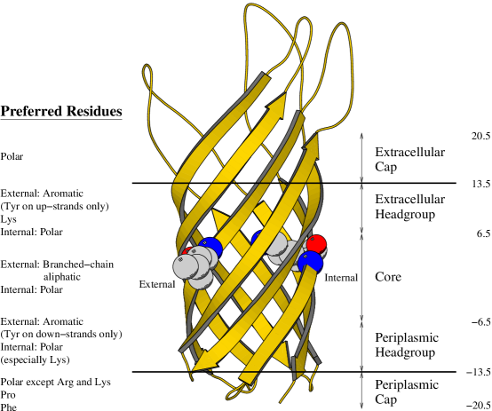
Figure 1: Definitions of boundaries of regions and summary of residue region-specific preferences shown on the structure of the 8-strand barrel of OmpA. Regions, defined by distance from the barrel center, are defined as follows: Extracellular Cap = 13.5 Å to 20.5 Å  Extracellular Headgroup = 6.5 Å to 13.5 Å  Core = $-6.5$ Å to 6.5 Å  Periplasmic Headgroup = $-13.5$ Å to $-6.5$ Å  Periplasmic Cap = $-20.5$ Å to $-13.5$ ÅṖreferred residues (those with high odds ratios) in each region are listed on the left. For reference, one internal residue (Lys 12, on the right) and one external residue (Leu 79, on the left) are shown.

We define eight distinct spatial regions for each TM strand based on the vertical distance along the membrane normal and the orientation of the side-chain (inside-facing or outside-facing, Figure 1). After placing the origin of the reference frame at the midpoint of the membrane bilayer and taking the vertical axis perpendicular to the bilayer as the $z$-axis, we measure the vertical distance of each residue from the barrel center (the $xy$ plane where $z=0$) along the $z$-axis. We follow the definition of Wimley [14] and define the core region as all residues whose $\alpha$-carbons are within 6.5 Å of the barrel center. The periplasmic and extracellular headgroup regions are similarly defined for the space 6.5-13.5 Å away from the barrel center on either side of the core region. These two headgroup regions are distinguished based on information in the original paper of the protein structure. Usually, both the N- and C-termini of the peptide chain as well as the short loop regions are found on the periplasmic side of the $\beta$-barrel. The core and two headgroup regions are further divided into internal and external residues, depending on whether their side-chains face into or away from the center of the barrel, respectively. The periplasmic and extracellular cap regions are defined as the space 13.5-20.5 Å away from the barrel center. These cap regions are similar to the membrane-water interface studied by Granseth et al. [22]. Since the cap regions are not located in the membrane domain, they are not divided into internal and external regions.

2.1.2 Region specific single-body propensities

	Periplasmic Cap		Periplasmic Headgroup				Core
Amino			Internal		External		Internal
Acid	Odds	$p$-Value	Odds	$p$-Value	Odds	$p$-Value	Odds	$p$-Value
A	0.72	2.4$\times 10^{-2}$	0.57	2.2$\times 10^{-2}$	0.61	3.1$\times 10^{-2}$	1.03	–
R	0.61	2.3$\times 10^{-2}$	1.62	3.4$\times 10^{-2}$	0.00	7.7$\times 10^{-7}$	1.77	3.2$\times 10^{-5}$
N	1.51	1.3$\times 10^{-3}$	1.45	–	0.32	7.5$\times 10^{-4}$	1.01	–
D	1.83	6.5$\times 10^{-8}$	1.33	–	0.05	1.8$\times 10^{-8}$	0.73	–
C	–	–	–	–	–	–	–	–
Q	0.52	4.6$\times 10^{-3}$	1.28	–	0.82	–	1.39	3.5$\times 10^{-2}$
E	1.20	–	1.61	4.3$\times 10^{-2}$	0.00	1.4$\times 10^{-6}$	1.73	1.1$\times 10^{-4}$
G	1.20	4.7$\times 10^{-2}$	0.58	4.0$\times 10^{-3}$	0.67	2.1$\times 10^{-2}$	1.68	5.9$\times 10^{-11}$
H	0.59	–	1.53	–	2.61	4.9$\times 10^{-3}$	0.70	–
I	0.74	–	0.53	–	1.90	3.5$\times 10^{-3}$	0.37	1.9$\times 10^{-4}$
L	0.86	–	0.49	5.4$\times 10^{-3}$	1.65	1.0$\times 10^{-3}$	0.42	1.9$\times 10^{-7}$
K	0.86	–	2.37	2.3$\times 10^{-5}$	0.16	3.2$\times 10^{-4}$	1.16	–
M	0.89	–	0.38	–	0.53	–	0.88	–
F	1.41	1.6$\times 10^{-2}$	0.13	3.1$\times 10^{-5}$	2.70	6.8$\times 10^{-10}$	0.39	2.7$\times 10^{-5}$
P	2.79	1.2$\times 10^{-10}$	1.03	–	0.27	3.7$\times 10^{-2}$	0.07	2.8$\times 10^{-6}$
S	0.94	–	1.78	5.0$\times 10^{-4}$	0.39	8.3$\times 10^{-4}$	1.33	1.6$\times 10^{-2}$
T	0.98	–	1.80	3.4$\times 10^{-4}$	0.77	–	1.14	–
W	0.82	–	0.41	–	2.54	1.5$\times 10^{-4}$	0.50	2.8$\times 10^{-2}$
Y	0.24	2.1$\times 10^{-10}$	0.51	1.7$\times 10^{-2}$	2.46	5.2$\times 10^{-10}$	0.95	–
V	0.65	1.2$\times 10^{-2}$	0.38	2.3$\times 10^{-3}$	1.85	2.6$\times 10^{-4}$	0.30	2.0$\times 10^{-8}$
	Core		Extracellular Headgroup				Extracellular Cap
Amino	External		Internal		External
Acid	Odds	$p$-Value	Odds	$p$-Value	Odds	$p$-Value	Odds	$p$-Value
A	1.95	2.8$\times 10^{-13}$	0.81	–	0.42	1.2$\times 10^{-3}$	1.00	–
R	0.07	1.0$\times 10^{-11}$	1.15	–	0.87	–	1.54	2.2$\times 10^{-4}$
N	0.13	4.7$\times 10^{-13}$	1.03	–	0.36	2.7$\times 10^{-3}$	1.56	7.0$\times 10^{-6}$
D	0.09	1.2$\times 10^{-15}$	1.11	–	0.76	–	1.53	6.5$\times 10^{-6}$
C	–	–	–	–	–	–	4.41	–
Q	0.14	3.1$\times 10^{-9}$	2.22	7.8$\times 10^{-5}$	1.23	–	1.18	–
E	0.00	5.4$\times 10^{-14}$	1.28	–	0.41	2.9$\times 10^{-2}$	1.32	3.3$\times 10^{-2}$
G	0.75	7.2$\times 10^{-3}$	1.15	–	0.39	1.7$\times 10^{-5}$	0.96	–
H	0.23	8.2$\times 10^{-3}$	0.25	–	2.61	8.1$\times 10^{-3}$	1.06	–
I	2.29	1.7$\times 10^{-10}$	0.79	–	1.00	–	0.60	5.2$\times 10^{-3}$
L	2.49	9.7$\times 10^{-29}$	0.65	–	0.89	–	0.51	1.4$\times 10^{-7}$
K	0.04	8.3$\times 10^{-12}$	0.75	–	1.21	–	1.54	3.6$\times 10^{-4}$
M	1.53	–	1.51	–	0.98	–	0.98	–
F	1.26	–	0.26	7.5$\times 10^{-4}$	1.89	1.3$\times 10^{-3}$	0.61	1.5$\times 10^{-3}$
P	1.11	–	0.00	1.4$\times 10^{-3}$	0.60	–	1.03	–
S	0.29	5.1$\times 10^{-10}$	1.48	2.7$\times 10^{-2}$	0.43	3.5$\times 10^{-3}$	1.30	5.2$\times 10^{-3}$
T	0.70	1.6$\times 10^{-2}$	1.55	1.2$\times 10^{-2}$	0.75	–	0.86	–
W	0.85	–	0.54	–	3.63	6.6$\times 10^{-9}$	0.57	1.8$\times 10^{-2}$
Y	1.11	–	0.75	–	2.91	6.2$\times 10^{-14}$	0.62	3.1$\times 10^{-4}$
V	2.65	4.9$\times 10^{-26}$	0.69	–	1.10	–	0.52	6.0$\times 10^{-6}$

Table 1: Single-body propensities by region with significance level measured by $p$-values. Odds ratio entries listed as “–” indicate that no residues of that type occurred in the region in the dataset. $p$-value entries listed as “–” are not significant at the threshold of 0.05.

Single-body propensities can be used to reflect the preference of different types of residues for different spatial regions of the transmembrane (TM) barrel. We define the single-body propensity of an amino acid residue type as an odds ratio comparing the frequency of this residue type in one region to its frequency in all eight regions combined. Results of residue single-body propensities are listed in Table 1, along with statistical significance in the form of $p$-values. These two-tailed $p$-values represent the probability that an odds-ratio will be more extreme than the observed one in the reference model, in which the positions of the residues in all proteins in the dataset are equally likely to take any one combination when they are exhaustively permuted.

2.1.3 Location preference of residues

Similar to previous studies [14], we find that aromatic residues have a strong preference for the external extracellular and periplasmic headgroup regions. Long aliphatic residues are favored in the external-facing core regions, and polar residues in all internal-facing regions as well as both cap regions. Cys residues do not occur in any TM region or the periplasmic cap region, consistent with earlier findings for helical membrane proteins [23]. The favorable propensity of Cys for the extracellular cap in Table 1 is due to a single cysteine cross-bridge in LamB (pdb 2mpr) and is not statistically significant.

We find that Pro prefers to be in the periplasmic cap region, because Pro residues are enriched in the short $\beta$-turns found in this region. Phe also prefers this region, despite its generally low propensity for $\beta$-turn regions [26]. While the $\alpha$-carbon of the Phe residue is situated in the periplasmic cap and therefore does not contribute to the TM $\beta$-sheet, the aromatic side-chain extends into the TM region and contributes to the “aromatic girdle” by “anti-snorkeling.” The preference of Phe for the periplasmic cap region has been described for both $\alpha$-helical [25] and $\beta$-barrel membrane proteins [27].

Our study provides novel insights about the location preferences of residues, as well as the significance of these preferences as measured by $p$-values (Table 1), which have not been provided in previous studies [14, 16]. We discuss several novel findings in more detail below.

The positive-outside rule: asymmetric distribution of basic residues in the cap regions.

The propensities for basic amino acids are very different between the periplasmic and extracellular cap regions. Arg and Lys have a lower preference for the periplasmic cap region (0.61 and 0.86 respectively) than for the extracellular cap regions (1.54 for both), despite the general “rule” that polar residues prefer both cap regions. Thus basic residues are more than twice as likely to be found in the extracellular cap than in the periplasmic cap. In contrast, acidic residues (Asp and Glu) are prevalent and evenly distributed in both cap regions. This pattern is analogous to the “positive-inside” rule for $\alpha$-helical membrane proteins, which states that acidic residues are evenly distributed at both ends of a TM helix, but basic residues favor the cis side of the membrane, i.e. the side in which the helix inserts [24]. Because $\beta$-barrel membrane proteins insert into the outer membrane from the periplasmic side [12], the asymmetric distribution of basic residues described here is the opposite of the positive-inside rule, and thus we have named it the “positive-outside” rule.

2.2 Strand interactions: pairwise spatial motifs and antimotifs

Single-residue propensities cannot capture information about interactions between residues on different strands. Little is known about whether there is any specific preference for residues to interact across adjacent strands. This is in contrast to helical membrane proteins, where helical interactions are the subject of several studies [23, 28, 29, 30, 31, 32].

2.2.1 Model of strand interactions: Strong H-bonds, side-chain interactions, and weak H-bonds

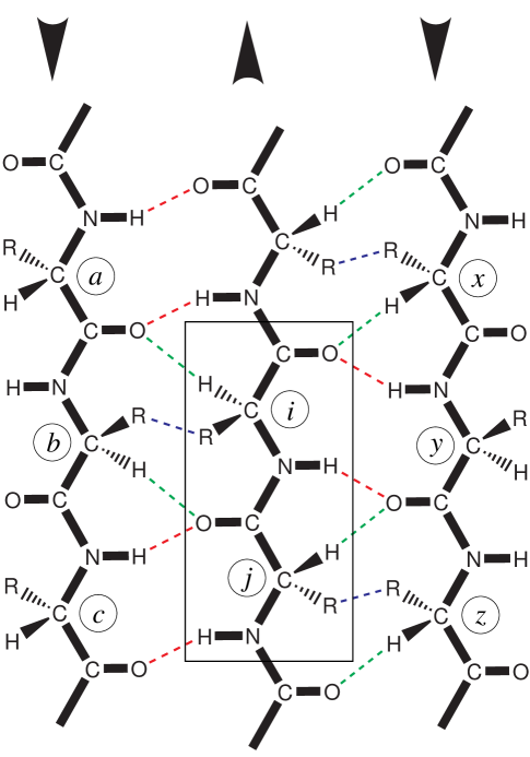
Figure 2: Repeating pattern of interstrand interactions and alternating internal and external side-chains. Red = strong H-bonds, Blue = non-H-bonded interactions, Green = weak H-bonds. Residues $i$ and $j$ in the center constitute one dyad (boxed). Residue $i$ interacts in a strong N-O H-bond with residue $y$ on its right and a non-H-bonded interaction with residue $b$ on its left. In contrast, residue $j$ interacts in a strong H-bond with residue $c$ on its left and a non-H-bonded interaction with residue $z$ on its right. This alternating dyad pattern repeats throughout each strand. In addition, each residue also interacts through weak C_α-O H-bonds to two residues, one on each side. In this case, $i$ shares a weak H-bond with both $a$ and $x$, and $j$ with both $b$ and $y$. Thus, residue $j$ interacts through weak H-bonds to the “bridge partners” (strong H-bond and non-H-bonded interactions, in this case $b$ and $y$) of the next residue in the strand, $i$, in the N-C direction (as shown by arrows at the top).

Strands in $\beta$-barrel membrane proteins have 7 or more residues with a clear internal face and external face. Interstrand interactions in antiparallel $\beta$-sheets are characterized by a periodic dyad bonding repeat pattern, which consists of units of two residues (Figure 2). We characterize interstrand pairwise interactions with three different types of interactions, namely, strong regular hydrogen bonds between backbone N and O atoms, “non-H-bonded” side-chain interactions (interactions without strong backbone N-O hydrogen bonds), and weak C_α-O hydrogen bonds between the C_α atom of one residue and a backbone oxygen on another strand. These three interstrand interactions occur periodically and are depicted in Figure 2.

The strong N-O hydrogen bonds occur between residues on adjacent strands. The non-H-bonded interactions alternate with the strong hydrogen bonds along adjacent $\beta$-strands. The weak C_α-O hydrogen bonds are displaced one residue along adjacent $\beta$-strands. Recent studies by Ho and Curmi on soluble $\beta$-sheets have shown that these weak hydrogen bonds have a significant impact on the arrangement of residues on adjacent strands, such that bonded residues are not immediately across from each other, but slightly displaced along the axis of the strand [33]. This effect may be responsible for the twisting of $\beta$-sheets. The role of weak C_α-O H-bonds has also been well studied in helical membrane proteins [34].

The three types of interactions used in this study are defined by their relationship to the backbone hydrogen-bonding pattern in $\beta$-sheets. Unless otherwise specified, we use “strong H-bond” to refer to a pair of residues that share strong N-O backbone H-bonds, “non-H-bonded interaction” to a pair of residues on adjacent strands that interact but do not share backbone H-bonds, and “weak H-bond” to a pair of residues that share weak C-O backbone H-bonds (Figure 2).

2.2.2 Interstrand pairwise interaction propensity, spatial motifs and antimotifs

We study interstrand interactions to identify spatial patterns in the form of pairing residues across strands with a strong preference to form hydrogen bonds, non-H-bonded interactions, and weak C_α-O hydrogen bonds. We calculate TransMembrane Strand Interaction Propensity (Tmsip) scales, which are the values of odds ratios comparing the observed frequency of interstrand contact interactions to the expected frequency. Among these contact interactions, we define spatial motifs as two-body interactions whose propensity is greater than 1.2 (i.e. favored) and statistically significant, and spatial antimotifs as two-body interactions whose propensity is less than 0.8 (i.e. disfavored) and statistically significant. Table 2 lists the Tmsip values and the $p$-values of motifs and antimotifs for each interaction type (strong H-bonds, non-H-bonded interactions, and weak H-bonds) at the significance level of $p<0.05$. A full list of all residue pairs is included in Supplementary Material.

(a) Motifs
Strong H-Bonds						Non-H-Bonded Interactions						Weak H-Bonds
Pair	Obs.	Exp.	Odds	$p$-Value		Pair	Obs.	Exp.	Odds	$p$-Value		Pair	Obs.	Exp.	Odds	$p$-Value
GY	39	25.0	1.56	8.0$\times 10^{-4}$		WY	22	8.1	2.71	4.1$\times 10^{-7}$		DT	17	8.3	2.05	2.2$\times 10^{-3}$
ND	10	3.6	2.76	1.2$\times 10^{-3}$		GI	16	9.0	1.77	1.2$\times 10^{-2}$		GP	12	6.8	1.78	1.3$\times 10^{-2}$
GF	18	10.0	1.80	4.7$\times 10^{-3}$		RE	12	6.4	1.87	1.3$\times 10^{-2}$		EM	6	2.6	2.31	3.5$\times 10^{-2}$
IY	18	10.1	1.79	4.8$\times 10^{-3}$		GV	22	13.7	1.60	1.6$\times 10^{-2}$		DP	5	2.0	2.52	3.9$\times 10^{-2}$
KS	12	6.2	1.95	1.2$\times 10^{-2}$		QG	19	12.1	1.57	2.3$\times 10^{-2}$
LW	10	5.2	1.92	2.5$\times 10^{-2}$		LL	24	16.7	1.44	2.7$\times 10^{-2}$
LY	34	24.7	1.37	2.9$\times 10^{-2}$		AV	29	20.9	1.39	3.7$\times 10^{-2}$
RP	3	0.8	4.00	3.1$\times 10^{-2}$		LP	8	3.9	2.07	3.7$\times 10^{-2}$
AA	16	10.6	1.50	4.8$\times 10^{-2}$
HK	3	0.9	3.33	5.0$\times 10^{-2}$
(b) Antimotifs
Strong H-Bonds						Non-H-Bonded Interactions						Weak H-Bonds
Pair	Obs.	Exp.	Odds	$p$-Value		Pair	Obs.	Exp.	Odds	$p$-Value		Pair	Obs.	Exp.	Odds	$p$-Value
YY	3	10.6	0.28	3.7$\times 10^{-3}$		GK	3	9.4	0.32	1.0$\times 10^{-2}$		PT	0	3.7	0.00	1.6$\times 10^{-2}$
						QV	0	4.2	0.00	1.7$\times 10^{-2}$		AT	22	33.2	0.66	1.9$\times 10^{-2}$
						GY	14	22.7	0.62	2.7$\times 10^{-2}$		FV	1	5.3	0.19	2.6$\times 10^{-2}$
						NL	2	6.1	0.33	4.6$\times 10^{-2}$

Table 2: Pairwise interstrand spatial motifs and antimotifs with propensities and $p$-values by interaction type. Only motifs significant at the threshold $p$-value of 0.05 are listed. Obs. = observed number of pairs, Exp. = expected number of pairs calculated as described in methods.

For strong backbone H-bond interactions, small residues and aromatic residues often have a strong propensity to interact, such as G-Y and G-F. Polar-polar residue interactions are also strongly favored, including N-D and K-S. In addition, branched hydrophobic residues and aromatic residues frequently form spatial motifs (I-Y, L-W, and L-Y). In contrast, aromatic-aromatic interactions are strongly disfavored for strong H-bond interactions: Y-Y is an antimotif, and W-Y is also strongly disfavored (propensity 0.21, $p$-value 0.06). This likely reflects the effects of bulky aromatic side-chains.

For non-backbone-H-bonded interactions, the W-Y motif stands out as the one with the most significant $p$-value among all spatial motifs (propensity 2.71, $p$-value 4$\times 10^{-7}$). Small residues form spatial motifs with branched residues and Gln (G-I, G-V, Q-G, and A-V). Other motifs of non-H-bonded interactions involve Leu (L-L and L-P).

Weak H-bond interactions have fewer spatial motifs. These involve charged residues (D-T, E-M, and D-P), or Pro residues (G-P and D-P).

2.2.3 Propensity and spatial motifs using a reduced alphabet

As seen in Table 2, residues of similar shape or physicochemical properties often behave similarly in forming high propensity spatial interactions. It is known that a reduced alphabet of fewer than 20 types of amino acid residues is often adequate for a protein to perform its biological functions [35], for computational recognition of homologous protein sequences [36], and for recognition of native structures from decoys [37]. A reduced alphabet would also be useful for statistical studies using limited data, as it would increase statistical significance for groups of related amino acids.

Figure 3: Clustering of residues based on single and pairwise propensities. G and P are assigned to their own clusters. The remaining three clusters are Polar (N, D, H, C, M, R, K, Q, T, E, and S), Aliphatic (A, I, L, and V), and Aromatic (Y, F, and W).

To further understand the nature of interstrand propensity and spatial motifs, we recalculated interstrand propensity using a simplified amino acid alphabet. An objective way to obtain a reduced alphabet is to group amino acids with similar location preference and strand pairing propensities. We cluster amino acids using the results obtained in the single and two-body studies, as described in Supplementary Material. The resulting clusters forming the reduced alphabet (Figure 3) are as follows: Gly by itself, Pro by itself, polar residues (Arg, Asn, Asp, Cys, Gln, Glu, His, Lys, Met, Ser, and Thr), aliphatic residues (Ala, Ile, Leu, and Val), and aromatic residues (Phe, Trp, and Tyr). Odds ratios and $p$-values were then obtained for strand interactions between residue clusters using the same method for the full amino acid alphabet. Table 3 summarizes the results obtained using this reduced alphabet.

		Strong H-Bonds					Non-H-Bonded					Weak H-Bonds
Pair		Obs.	Exp.	Odds	$p$-Value		Obs.	Exp.	Odds	$p$-Value		Obs.	Exp.	Odds	$p$-Value
Gly-Gly		16	19.7	0.81	–		14	17.8	0.78	–		34	34.4	0.99	–
Gly-Pro		3	1.1	2.77	–		3	2.9	1.05	–		12	6.8	1.78	1.3$\times 10^{-2}$
Gly-Polar		100	115.0	0.87	2.7$\times 10^{-2}$		122	118.5	1.03	–		142	161.4	0.88	2.0$\times 10^{-2}$
Gly-Aliph.		68	68.6	0.99	–		87	68.1	1.28	2.1$\times 10^{-3}$		230	208.5	1.10	1.8$\times 10^{-2}$
Gly-Arom.		62	40.9	1.52	2.5$\times 10^{-5}$		26	40.8	0.64	2.6$\times 10^{-3}$		84	90.6	0.93	–
Pro-Pro		0	0.0	–	–		0	0.6	0.00	–		0	0.0	–	–
Pro-Polar		8	4.6	1.74	–		7	7.4	0.95	–		15	18.3	0.82	–
Pro-Aliph.		3	8.6	0.35	5.3$\times 10^{-3}$		15	10.1	1.49	–		8	9.3	0.86	–
Pro-Arom.		4	3.7	1.09	–		4	7.4	0.54	–		3	3.6	0.83	–
Polar-Polar		228	204.9	1.11	1.1$\times 10^{-4}$		239	210.5	1.14	8.6$\times 10^{-6}$		223	216.5	1.03	–
Polar-Aliph.		167	178.2	0.94	–		122	182.3	0.67	2.1$\times 10^{-11}$		662	677.1	0.98	–
Polar-Arom.		67	90.3	0.74	2.6$\times 10^{-4}$		99	98.7	1.00	–		344	319.1	1.08	1.5$\times 10^{-2}$
Aliph.-Aliph.		140	144.7	0.97	–		182	152.5	1.19	3.4$\times 10^{-6}$		166	162.6	1.02	–
Aliph.-Arom.		158	131.1	1.20	5.1$\times 10^{-4}$		119	141.5	0.84	6.1$\times 10^{-3}$		155	164.8	0.94	–
Arom.-Arom.		23	35.5	0.65	2.3$\times 10^{-3}$		62	41.8	1.48	1.4$\times 10^{-5}$		34	37.9	0.90	–

Table 3: Odds ratios for interstrand residue pairs using a reduced amino acid alphabet. Residue clusters forming the reduced alphabet are defined in Figure 3. $p$-value entries listed as “–” were not significant at the threshold of 0.05. Aliph. = Aliphatic, Arom. = Aromatic, Obs. = observed number of pairs, Exp. = expected number of pairs calculated as described in methods.

Several general patterns emerge. The most dramatic differences in strand pairing between different types of interactions are those between strong H-bonds and non-H-bonded interactions. Gly-Aromatic and Aliphatic-Aromatic pairs have much higher preferences for strong H-bonds than for non-H-bonded interactions, while Aromatic-Aromatic and Gly-Aliphatic pairs have higher preferences for non-H-bonded interactions. Smaller differences are detected for Polar-Aliphatic pairs (higher in strong H-bonds) and for Polar-Aromatic and Aliphatic-Aliphatic pairs (higher in non-H-bonded interactions). Weak H-bond interactions did not show very strong preferences in this analysis, except for the G-P pair already reported in Table 2.

The high-propensity Aromatic-Aromatic non-H-bonded interactions include W-Y, the highest-propensity pairwise spatial motif. An example of the W-Y motif (Figure 4a) may help to explain why this family of interactions has such high propensity. The Tyr and Trp residues involved in this motif often align their side-chains to maximize contact between their aromatic rings and between their polar groups. At the same time, the bulky side-chains cause steric hindrance preventing direct backbone N-O hydrogen bonds, and thus these pairs are disfavored in strong backbone H-bond interactions.

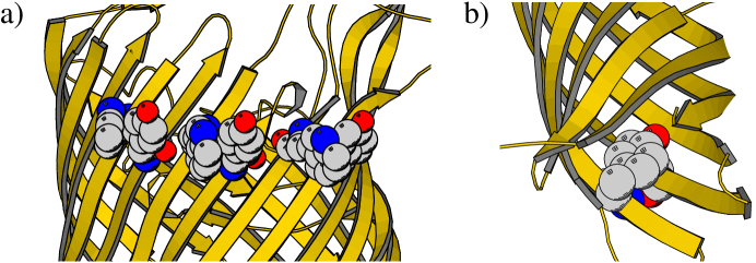
Figure 4: Two examples of interstrand spatial motifs in $\beta$-barrel membrane proteins: a) An instance of the WY non-H-bonded interaction motif in LamB. The aromatic side-chains of Trp and Tyr show considerable contact interaction. b) An instance of the GY strong H-bonded interaction motif in NspA. The protein has been tilted to show the motif on the internal side of the barrel. The aromatic side-chain of Tyr interacts with the Gly residue on the adjacent strand. This is an example of “aromatic rescue.”

2.2.4 Internal and external preference of pairwise interactions

We find that there are clear preferences for some residue pairs to face either the outside or inside of the barrel. Pairs of bulky aromatic residues (Phe, Tyr, and Trp) are almost always on the outside of the barrel, due to the steric hindrance in the barrel interior that would result. All 26 of the strong H-bonded Aromatic-Aromatic interacting pairs occur on the outside of the barrel, as do 55 of the 62 Aromatic-Aromatic pairs that form non-H-bonded interactions. The preference of Gly-Gly pairs to face the inside of the barrel is also significant for non-H-bonded interacting pairs (17 out of 19 occur on the inside). However, no clear preference is seen for Gly-Gly strong H-bonds: Only 8 of 16 pairs occur on the inside. For strong H-bonded pairs between Gly and aromatic residues, 48 out of 63 pairs are internal, whereas there is no preference for non-H-bonded pairs (14 out of 25 are internal). This may reflect a preference for “aromatic rescue” of Gly, discussed below. The orientation for weak H-bonded pairs is not relevant, since one residue always faces the inside of the barrel and the other always faces the outside, as shown in Figure 2.

2.2.5 Comparison to soluble barrel and barrel-like $\beta$-sheets

In order to determine whether the pairwise propensities calculated for TM $\beta$-barrels were due to the effects of the transmembrane environment or due to the intrinsic structural effects of $\beta$-barrels, we calculated pairwise propensities for a set of soluble $\beta$-barrels and barrel-like $\beta$-sheets that were structurally similar to the TM $\beta$-barrel dataset as determined by the Combinatorial Extension structural alignment method [38]. The soluble dataset contains 28 proteins. All of the proteins contain anti-parallel $\beta$-sheets with a right-hand twist, similar to TM $\beta$-barrels. Some open $\beta$-barrels and other $\beta$-sheets were included to ensure that the size of the dataset would be similar to that of the TM $\beta$-barrels. The final dataset has approximately the same number of strand pairs, though about 40% fewer residue pairs. Significant pair propensities for the soluble $\beta$-sheet dataset for each interaction type are listed in Supplementary Material.

Only two motifs appear in both TM and soluble proteins: G-V non-bonded pairs (propensity 1.60 in TM $\beta$-barrels, 1.78 in soluble $\beta$-sheets) and G-P weak H-bonds (1.78 TM, 3.75 soluble). In soluble $\beta$-sheets, polar-polar and hydrophobic-hydrophobic pairs have high propensities for strong H-bond and non-H-bonded pairings, while polar-hydrophobic pairs have low propensities. The results for weak H-bonds show an opposing trend. The strongest motifs in TM $\beta$-barrels, W-Y non-H-bonded pairs and G-Y strong H-bonds, are not statistically significant in soluble sheets. W-Y non-H-bonded pairs have propensity 1.06 and G-Y strong H-bonds have propensity 1.27 with $p$-value 0.55.

Pairwise interhelical interactions in TM $\alpha$-helical membrane proteins have also been studied using odds ratios [23]. The only favorable interaction motif found in both TM $\alpha$-helices and TM $\beta$-barrels is G-F, a strong H-bond motif (odds ratio 1.80) involved in aromatic rescue. Otherwise, there are very few similarities between the two protein families.

2.3 Prediction of strand register

The single and pairwise propensities can be useful for structure prediction. We have developed an algorithm to predict strand register in $\beta$-barrel membrane proteins knowing only amino acid sequences and the approximate positions of the first residue in each strand. The latter can be obtained by several strand predictors, though they cannot themselves predict strand register. We use the hidden Markov model predictor of Bigelow et al. [7]. We also test our method when the actual strand starts are given beforehand.

Our predictor consists of two steps. In step 1, we use the single-body regional propensities to refine the approximate strand starts given by the HMM predictor into “true” strand starts. It is only necessary for the strand predictor to predict strand starts within 5 residues of the exact strand start. In step 2, we use the two-body interstrand propensities (Tmsip) to predict final strand register for each strand pair. Details of the algorithm are discussed in Methods.

Method		Strands	Accuracy
Full prediction		112	44%
Step 1 only		100	39%
Step 2 only		92	36%
No prediction		61	24%
Random		17	7%

Table 4: Prediction of strand register in $\beta$-barrel membrane proteins. We report the success of our tests as the number of strand pairs whose register is correctly predicted (“Strands”) and the proportion out of the 256 strand pairs tested (“Accuracy”). Listed are the accuracies for using both steps (single and pairwise propensities) as described in Methods (“Full prediction”), using step 1 or 2 individually, skipping both steps (“No prediction”), or using randomly generated strand registers (“Random”).

The results of our predictor are reported in Table 4, where the proportion of strand pairs (out of 256) whose register is correctly predicted is listed. When the strand starts predicted by the method of Bigelow et al. are given as input, the accuracy is 44%. When the actual strand starts from the PDB structures are given as input instead, the accuracy is 46%. This shows that only approximate strand starts are necessary for strand registration prediction.

We compare our accuracy to a random control, in which we randomly select a window from the 11 available positions for each strand and then randomly select a strand shear from the 11 possible values for each strand pair (as described in Methods). We ran this random selection 10 times on the dataset, and only 17.4 strand pairs were predicted on average (standard deviation 3.61). This translates to a random accuracy of 7%. Our accuracy of 44% is thus considerably better than random.

We also compare our results to a similar prediction of strand register in soluble $\beta$-sheets by Steward and Thornton [19]. This prediction uses the sum of single and pairwise scores to align one $\beta$-strand against a fixed strand that it is known to pair with, and achieves an accuracy of 31% in antiparallel $\beta$-sheets. These conditions are similar to ours when the actual strand starts are given as inputs and we skip step 1. We achieve an accuracy of 68% in TM $\beta$-barrels under these conditions.

3 Discussion

We have described residue preferences for different regions and a number of spatial patterns for $\beta$-barrel membrane proteins. Many of the novel patterns discovered in this study provide useful information about the assembly and folding process of $\beta$-barrel membrane proteins.

“Positive-outside” rule.

Basic residues have an asymmetric distribution between the two cap regions of $\beta$-barrel membrane proteins. Arg and Lys have propensities of 0.61 and 0.86 in the periplasmic cap region, respectively, but 1.54 and 1.54 in the extracellular cap region, and thus have over twice the preference to be found in the extracellular cap region than in the periplasmic cap region. This is notable for several reasons: first, one would intuitively expect charged residues to have high propensity in both cap regions, since they are surrounded by an aqueous environment; second, acidic residues have high and relatively similar propensities in both cap regions (Asp has a propensity of 1.83 for the periplasmic cap and 1.53 for the extracellular cap, and Glu has 1.20 and 1.32 for these regions, respectively); third, despite their poor propensity for the periplasmic cap, basic residues have very high propensities for the internal face of the periplasmic headgroup region (Arg 1.62, Lys 2.37), and often “snorkel” away from the center of the lipid bilayer and extend into the periplasmic space.

A similar asymmetric distribution of basic residues in cap regions has been found in $\alpha$-helical membrane proteins, yet the distribution is reversed: Basic residues have a high propensity for the inner, cytoplasmic cap, and a low propensity for the outer cap (facing the extracellular space in eukaryotes and gram-positive bacteria or facing the periplasm in gram-negative bacteria) [24]. This property was named the “positive-inside” rule. By analogy, $\beta$-barrel membrane proteins thus show a “positive-outside” rule.

A possible explanation for this result is that the asymmetric distribution of basic residues is related to the asymmetric lipid composition of the outer membrane. The inner leaflet of the outer membrane, which faces the periplasm, is composed primarily of phosphatidylethanolamine (PE), while the outer leaflet, which faces the extracellular environment, has a high concentration of lipopolysaccharide (LPS), which bears several negatively charged groups. The asymmetric distribution of basic residues within the protein may lead to a stable positioning of the protein within this asymmetric lipid bilayer. It has been suggested that $\beta$-barrel membrane proteins may interact with LPS in the periplasm before co-inserting into the outer membrane [42]. If this is true, the high propensity of basic residues on the extracellular side of the protein would attract the highly negatively-charged LPS so that the protein will insert in the correct direction. In a recent study in which the structure of the TM $\beta$-barrel of FhuA is co-crystallized with one LPS molecule, LPS binds strongly to basic residues on FhuA in the extracellular cap region, forming hydrogen bonds or ionic interactions [43, 44]. Another study suggests that the frequency of positively charged residues in the headgroup region is correlated to in vitro affinity of $\beta$-barrel membrane proteins for different phospholipids. [45]. Thus, the affinity of the two sides of the barrel for the two outer membrane leaflets may be affected by the amino acid composition of the barrel and the lipid composition of the leaflets.

Aromatic rescue of glycine in $\beta$-barrel membrane proteins.

Tyr-Gly is the most favorable interstrand motif for backbone H-bond interactions (propensity 1.56, $p$-value 8$\times 10^{-4}$). Of the 39 G-Y strong H-bonded pairs in the dataset, 32 are on the inside of the barrel, where Tyr is normally disfavored. Tyr adopts an unusual rotamer (60,90) in this location: 60% of internal Tyr side-chains adopt this rotamer, while only 8% of external Tyr side-chains and 6% of Tyr side-chains in soluble $\beta$-strands do [40]. There is a single explanation for this rotamer preference and the unusual preference of Tyr for the inside of the barrel when it is part of a G-Y interaction. As shown in Figure 4b, the side-chain of Tyr has extensive contacts with and covers the Gly residue to which it is backbone H-bonded. Of the 32 internal G-Y strong H-bonded pairs, 30 show this behavior, but only 1 of 7 external G-Y pairs do.

Merkel and Regan discovered the same behavior in soluble $\beta$-sheets, and named it “aromatic rescue” of glycine [20]. They found that aromatic rescue mitigates the instability Gly causes in $\beta$-sheets. They proposed that the aromatic side-chain prevents the exposure of the backbone around Gly to solvent while at the same time minimizing the surface area of the aromatic ring exposed to solvent. This effect also accounts for the fact that this pattern occurs preferentially on the inside of the barrel in TM regions, where it is exposed to solvent or a polar environment. Phe behaves similarly to Tyr in this region. G-F is a significant strong H-bonded motif (propensity 1.80, $p$-value 5$\times 10^{-3}$) and displays aromatic rescue on the inside of the barrel. Likewise, the (60,90) rotamer is observed in 83% of internal Phe side-chains, but only in 19% of external Phe side-chains and 5% of Phe side-chains in soluble $\beta$-strands [40].

Hutchinson et al. studied the relationship between H-bonded and non-H-bonded pairs in soluble $\beta$-sheets, and found that G-F H-bonds were 2.63 times more likely than G-F non-H-bonded pairs [21]. This is similar to the ratio for TM $\beta$-barrels (2.37). However, the ratio of G-Y for TM $\beta$-barrels (2.93) is considerably higher than that for soluble $\beta$-sheets (1.39). Tyr may have a much larger role in aromatic rescue in TM $\beta$-barrel membrane proteins than soluble $\beta$-sheets because of the higher polarity of Tyr side-chains compared to Phe. Aromatic rescue may be even more important for the internal surface of TM $\beta$-barrels than for soluble $\beta$-sheets, both because of the need to have polar residues such as Tyr on the internal surface and the need to have Gly in order to relieve the steric pressure caused by the curvature of the barrel.

Structure prediction.

We have incorporated our propensity values into a preliminary study predicting strand pair register in TM $\beta$-barrels. We find that our predictor can achieve significantly higher accuracy than random. It can achieve nearly the same accuracy by inputting strand starts approximated by the hidden Markov model predictor of Bigelow et al. [7] as when the true strand starts are known. Thus, only the amino acid sequence is necessary for strand pairing prediction if the method of Bigelow et al. is used first. Our accuracy is considerably better than random (44% vs. 7%), and is also better than just relying on the initial HMM prediction (24%). The predictor discussed in this study represents the first step towards a full structure prediction of TM $\beta$-barrels.

We also assessed the effects of using only knowledge of strand starts (step 1) or only strand pairing (step 2). We can skip step 1 by not refining the strand starts given as input (“Step 2 only” in Table 4). We find that the accuracy of the predictor decreases to 36% using start positions from the HMM predictor. This shows that the single-body regional preferences improve accuracy by 8%. We can skip step 2 (“Step 1 only” in Table 4) by not using our pairwise interstrand propensities, and simply assigning the most frequently observed strand register as correct. In this case, the accuracy decreases to 39%. Clearly, both steps 1 and 2 are necessary to achieve maximal accuracy. When both steps 1 and 2 are skipped (“No prediction” in Table 4), the accuracy drops to 24%.

Determining factors of folding and assembly.

There are two main factors that determine the spatial patterns described in this study. As with $\alpha$-helical membrane proteins, the folding and assembly of $\beta$-barrel membrane proteins in the transmembrane region are governed by the thermodynamics of lipids and proteins and their interactions. On the other hand, the sorting and targeting process required for integrating membrane proteins into lipid bilayers in the correct direction after biosynthesis is an important process of the cell, and involves complex biomolecular machinery [12]. For helical membrane proteins, the nature of such machinery is being uncovered by the study of translocons [47]. For $\beta$-barrel proteins, recent work on chaperone-assisted folding hint at a very complex machinery as well [12].

Distinguishing spatial patterns due to fundamental thermodynamics from those due to the unique requirements of biological localization is a challenging task. The identification and understanding of the origins of these motifs will help to elucidate the folding mechanisms of $\beta$-barrel proteins. An attractive hypothesis is that these two types of events can be discerned from further analysis of propensities, motifs, and antimotifs.

Experimentally testable hypotheses.

The identification of favorable pairing residues may be useful for suggesting experimental studies to elucidate determinants important for in vivo folding and to dissect the determinants of thermodynamic stability for $\beta$-barrel membrane proteins. For example, Arg and Lys can be introduced in the periplasmic cap region, and if such mutants can fold with similar stability in in vitro experiments, this would suggest that the “positive-outside” rule may be important mostly for in vivo folding. In addition, measurement of the thermodynamic stabilities of $\beta$-barrel proteins in reconstituted lipid bilayers of different composition can help to clarify whether the origin of the “positive-outside” rule is due to the asymmetric composition of phospholipid bilayers.

Gly-Tyr interstrand pairs involved in aromatic rescue may serve as anchoring sites of $\beta$-barrel membrane protein folding. To study details of the folding mechanism, one could remove and add anchoring Gly-Tyr residue pairs at strategic positions simultaneously in order to introduce maximal changes in the effective contact orders, which would significantly alter the zipping process of folding [49]. Folding rate studies of these mutated proteins would be valuable for elucidating the folding mechanism of $\beta$-barrel proteins in general and the role of the high-propensity Gly-Tyr interaction in particular. The motifs, antimotifs, and spatial high propensity pairing described in this study can be used profitably for studying the folding and assembly mechanism of $\beta$-barrel membrane proteins.

Importance of statistical analysis for small datasets.

Previous studies of residue pairing in soluble $\beta$-sheets either lack a statistical model and hence provide no statistical significance in their results, or use simple models such as the $\chi^{2}$ test for $p$-value calculation, which is inappropriate for studying the pairing of very short strands [19, 18, 21].

Because no existing textbook or published statistical models are applicable for analyzing short strand pairing, the key component of our method is the development of methods of exact calculation of $p$-values for the null model of exhaustive permutation of strand sequences. With the development of a higher-order generalized hypergeometric model based on the combinatorics of short sequences, we are able to identify very significant motifs and antimotifs from very limited data. The development of rigorous statistical methods is an important technical development of work reported in this paper.

4 Model and Methods

We sketch briefly our models and computational methods below. More details can be found in Supplementary Material).

Database.

The dataset used to derive the statistical models comprises 19 $\beta$-barrel membrane proteins found in the Protein Data Bank (Table 5), totaling 262 $\beta$-strands. All proteins share no more than 26% pairwise sequence identity. All structures have a resolution of 2.6 Å or better.

Protein	Organism	Architecture	Strands	PDB ID
OmpA	E. coli	monomer	8	1BXW [51]
OmpX	E. coli	monomer	8	1QJ8 [52]
NspA	N. meningitidis	monomer	8	1P4T [53]
OpcA	N. meningitidis	monomer	10	1K24 [54]
OmpT	E. coli	monomer	10	1I78 [55]
OMPLA	E. coli	dimer	12	1QD6 [56]
NalP	N. meningitidis	monomer	12	1UYN [57]
Porin	R. capsulatus	trimer	16	2POR [58]
Porin	R. blastica	trimer	16	1PRN [59]
OmpF	E. coli	trimer	16	2OMF [60]
Omp32	C. acidovorans	trimer	16	1E54 [61]
LamB	S. typhimurium	trimer	18	2MPR [62]
ScrY	S. typhimurium	trimer	18	1A0S [63]
FepA	E. coli	monomer	22	1FEP [64]
FhuA	E. coli	monomer	22	2FCP [43]
FecA	E. coli	monomer	22	1KMO [65]
BtuB	E. coli	monomer	22	1NQE [66]
TolC	E. coli	trimer	4	1EK9 [67]
$\alpha$-Hemolysin	S. aureus	heptamer	2	7AHL [4]

Table 5: Dataset of 19 $\beta$-barrel membrane proteins used for this study. All proteins share no more than 26% pairwise sequence identity. Crystal structures have a resolution of 2.6 Å or less. Three identical chains of TolC and seven of $\alpha$-hemolysin form a single barrel; all other proteins listed form whole barrels with a single peptide chain.

The dataset of soluble barrel and barrel-like $\beta$-sheets was compiled by searching structural homologs using the Combinatorial Extension method [38] with each of the 19 proteins in the TM dataset. Because the resulting dataset was small, CE was used again on the two closed barrels obtained from the first attempt, streptavidin (pdb 1stp) and retinol binding protein (pdb 1brp). As with the TM dataset, all proteins share no more than 26% pairwise sequence identity. All structures have a resolution of 3.3 Å or better. The dataset comprises 28 soluble $\beta$-sheets: 1avg, 1ayr, 1bbp, 1bj7, 1bpo, 1brp, 1dfv, 1dmm, 1d2u, 1eg9, 1ei5, 1epa, 1em2, 1ewf, 1fsk, 1fx3, 1h91, 1jkg, 1lkf, 1m6p, 1qfv, 1std, 1stp, 1t27, 1una, 2a2u, 3blg, 4bcl.

Single-body propensities.

We define the single-body propensity $P_{r}(X)$ of residue type $X$ in region $r$ as the odds ratio comparing the frequency of a residue type in one region to its expected frequency when all eight regions are combined:

$$P_{r}(X)=\frac{f(X|r)}{\mathbb{E}[f^{\prime}(X|r)]},$$

where $f(X|r)$ is the observed frequency (number count) of residue type $X$ in region $r$, and $\mathbb{E}[f^{\prime}(X|r)]$ is the expected frequency of residue type $X$ in region $r$.

In order to calculate $\mathbb{E}[f^{\prime}(X|r)]$, we use a random null model of exhaustive permutation of all residues in all eight regions. Here each permutation occurs with equal probability. The probability $\mathbb{P}_{X|r}(i)$ of $i=f^{\prime}(X|r)$ residues of type $X$ being assigned to region $r$ follows a hypergeometric distribution: $\mathbb{P}_{X|r}(i)=h(i|n,n_{r},n_{x})=\binom{n_{x}}{i}\binom{n-n_{x}}{n_{r}-i}/\binom{n}{n_{r}},$ where $n$ is the number of residues of all types in all eight regions in the entire dataset, $n_{r}$ is the number of residues of all types in region $r$, and $n_{x}$ is the number of residues of type $X$ in all regions. The expected frequency of residue type $X$ occurring in region $r$ is the mean of the hypergeometric distribution $h(i|n,n_{r},n_{x})$:

$$\mathbb{E}[f^{\prime}(X|r)]=\sum_{i=0}^{n_{x}}i\cdot\mathbb{P}_{X|r}(i)=\frac{n_{r}\cdot n_{x}}{n}.$$ (1)

Therefore, the propensity $P_{r}(X)$ is:

$$P_{r}(X)=\frac{f(X|r)}{\mathbb{E}[f^{\prime}(X|r)]}=\frac{f(X|r)/n_{r}}{n_{x}/n}.$$

Because the frequency of occurrences of residues of type $X$ in region $r$ in the null model follows a hypergeometric distribution, we can calculate an exact $p$-value for an observed $f(X|r)$ to assess its statistical significance. We calculate a two-tailed $p$-value based on the null hypothesis that $P_{r}(X)=1.0$.

Determination of pairwise contacts.

The three types of pairwise contacts (strong H-bond, side-chain, and weak H-bond) were assigned for interacting residues based on contact types defined by the DSSP program (Definition of Secondary Structure of Proteins [50]) based on the atomic coordinates from PDB files. For $\beta$-sheets, DSSP defines bridge partners as residues across from each other on adjacent $\beta$-strands, and also determines whether bridge partners interact via backbone N-O H-bonds. Two TM residues on adjacent $\beta$-strands contribute to a backbone strong H-bond interaction if they are listed as bridge partners that contribute to backbone H-bonds. They contribute to a non-H-bonded interaction if they are listed as bridge partners but do not contribute to backbone H-bonds. They contribute to a weak H-bond if the residue with the smaller residue number (i.e. closer to the N-terminus of the protein) is a bridge partner to the residue immediately following the other residue of the pair. This is because a weak C_α-O H-bond extends by one residue in the N-C direction, as seen in Figure 2. Residues $j$ and $y$ contribute to a weak H-bond in Figure 2, for example, because the residue with the lower number ($y$, since it is closer to the N-terminus), is a bridge partner to $i$, the residue immediately following $j$. For a strand pair between the first and last strands of a protein, the larger and smaller numbered residues must be switched, to account for the fully circular nature of $\beta$-barrels. Residues outside the TM regions (core and headgroup) were not considered in our calculations of pairwise contacts.

Interstrand two-body spatial contact propensities.

The interstrand pairwise propensity (Tmsip) $P(X,Y)$ of residue types $X$ and $Y$ for each of the three types of pairwise contacts is given by:

$$P(X,Y)=\frac{f(X,Y)}{\mathbb{E}[f^{\prime}(X,Y)]},$$

where $f(X,Y)$ is the observed frequency of $X$-$Y$ contacts of a specific type in the TM regions (core and headgroup), and $\mathbb{E}[f^{\prime}(X,Y)]$ is the expected frequency of $X$-$Y$ contacts in a null model. In Tables 2 and 3, $f(X,Y)$ is listed under “Obs.”, and $\mathbb{E}[f^{\prime}(X,Y)]$ is listed under “Exp.”

In order to calculate $\mathbb{E}[f^{\prime}(X,Y)]$, we choose a null model in which residues within each of the two adjacent strands in a strand pair are permuted exhaustively and independently, and each permutation occurs with equal probability.

Contacts between residues of the same type. When $X$ is the same as $Y$, the probability $\mathbb{P}_{X,X}(i)$ of $i=f^{\prime}(X,X)$ number of $X$-$X$ contacts in a strand pair follows a hypergeometric distribution. $\mathbb{E}_{\rm all}[f^{\prime}(X,X)]$ is then the sum of the expected values of $f^{\prime}(X,X)$ for the set ${\cal SP}$ of all strand pairs in the dataset:

$$\mathbb{E}_{\rm all}[f^{\prime}(X,X)]=\sum_{sp\in{\cal SP}}\mathbb{E}[f^{\prime}_{sp}(X,X)]=\sum_{sp\in{\cal SP}}\frac{x_{1}(sp)\cdot x_{2}(sp)}{l(sp)},$$

where $x_{1}(sp)$ and $x_{2}(sp)$ are the numbers of residues of type $X$ in the first and second strand of strand pair $sp\in{\cal SP}$, respectively, and $l(sp)$ is the length of strand pair $sp$. The right-hand side is determined by using the expectation of the hypergeometric distribution, analogous to Equation (1). For statistical significance, two-tailed $p$-values can be calculated using $\mathbb{P}_{X,X}$.

Contacts between residues of different types. If the two contacting residues are not of the same type, i.e. $X\neq Y$, then the number of $X$-$Y$ contacts in the random model for one strand pair is the sum of two dependent hypergeometric variables, one variable for type $X$ residues in the first strand and type $Y$ in the second strand, and another variable for type $Y$ residues in the first strand and type $X$ in the second strand. The expected frequency of $X$-$Y$ contacts $\mathbb{E}[f^{\prime}(X,Y)]$ is the sum of the two expected values over all strand pairs $sp\in{\cal SP}$:

$$\mathbb{E}[f^{\prime}(X,Y)]=\sum_{sp\in{\cal SP}}\{\mathbb{E}[f^{\prime}_{sp}(X,Y)]+\mathbb{E}[f^{\prime}_{sp}(Y,X)]\}=\sum_{sp\in{\cal SP}}\{\frac{x_{1}(sp)\cdot y_{2}(sp)}{l(sp)}+\frac{y_{1}(sp)\cdot x_{2}(sp)}{l(sp)}\},$$

where $x_{1}(sp)$ and $x_{2}(sp)$ are the numbers of residues of type $X$ in the first and second strand, $y_{1}(sp)$ and $y_{2}(sp)$ are the numbers of residues of type $Y$ in the first and second strand, and $l(sp)$ is the length of strand pair $sp$. The right-hand side is determined by using the expectation of the hypergeometric distribution, analogous to Equation (1). A more complex hypergeometric formula for the null model is used for exact calculation of $p$-values (see details in Supplementary Material).

Strand register prediction.

Our algorithm consists of two steps, the prediction of exact strand starts and the prediction of strand register. In both steps, a probabilistic model is used which involves the summation of log-propensity values calculated in this study.

For step 1, we use the single-body regional propensities. We begin with an initial postion of strand start, e.g., as predicted by the hidden Markov model of Bigelow et al. [7], and sum the log-propensities of the surrounding amino acids for 11 windows: the window starting at the predicted strand start, and all windows within 5 residues from the original prediction. The window with the sum that reflects the highest probability is taken as the “true” strand start used in step 2.

For step 2, we use the pairwise two-body propensities. We begin with two adjacent strands, using the strand starts predicted in step 1. We then shift one strand against another, and sum the log-propensities of the surrounding residue pairs for 11 windows (called “strand shears”): the window in which the two strand starts are bonded together, and all windows within 6 residues up and 4 residues down for the original position. This is because a strand shear of +1 is the most commonly occurring strand shear in the dataset. The window with the sum that reflects the highest probability is taken as the correct strand pairing.

We exclude from our prediction analysis two proteins in our dataset (6 strand pairs) for which the HMM strand start predictor failed: TolC and $\alpha$-HL. This leaves our dataset with 17 proteins comprising 256 strands. We test our method in “leave-one-out” fashion, using 16 proteins to derive the log-propensity scores use to predict strand pairing in the 17th protein. The results are listed in Table 4.

5 Acknowledgment

We thank Dr. Bosco Ho for insightful comments. We thank Xiang Li, Drs. William Wimley and Jinfeng Zhang for helpful discussions. We thank Sarah Cheng for programming assistance. This work is supported by grants from the National Science Foundation (CAREER DBI0133856 and DBI0078270), National Institute of Health (GM68958), and Office of Naval Research (N000140310329).

6 Supplementary Material

This is a self-containing expaned section on methods.

Database.

The dataset used to derive the statistical models comprises 19 $\beta$-barrel membrane proteins found in the Protein Data Bank (Table 5), totaling 262 $\beta$-strands. All proteins share no more than 26% pairwise sequence identity. All structures have a resolution of 2.6 Å or better.

The dataset of soluble barrel and barrel-like $\beta$-sheets was compiled by searching structural homologs using the Combinatorial Extension method [38] with each of the 19 proteins in the TM dataset. Because the resulting dataset was small, CE was used again on the two closed barrels obtained from the first attempt, streptavidin (pdb 1stp) and retinol binding protein (pdb 1brp). As with the TM dataset, all proteins share no more than 26% pairwise sequence identity. All structures have a resolution of 3.3 Å or better. The dataset comprises 28 soluble $\beta$-sheets: 1avg, 1ayr, 1bbp, 1bj7, 1bpo, 1brp, 1dfv, 1dmm, 1d2u, 1eg9, 1ei5, 1epa, 1em2, 1ewf, 1fsk, 1fx3, 1h91, 1jkg, 1lkf, 1m6p, 1qfv, 1std, 1stp, 1t27, 1una, 2a2u, 3blg, 4bcl.

Spatial Regions and Strand Model.

In order to classify residues in $\beta$-barrel membrane proteins by specific spatial regions (core, headgroup, and polar caps), the coordinates in the protein’s PDB file were translated and rotated so that the $xy$-plane was perpendicular to the vertical axis of the barrel and equidistant to the observed aromatic girdles presumed to be at the membrane interfaces. An example of such a transformation is illustrated in Figure 1. Each residue in the protein was assigned a region based on the $z$-coordinate of its associated $\alpha$-carbon.

In addition, TM residues (those in the core or headgroup regions) were assigned as internal (i.e. their side-chains face into the center of the barrel) or external (i.e. their side-chains face away from the center of the barrel), depending on the angle between the vector from the barrel central axis to the $\alpha$-carbon and the vector from the $\alpha$-carbon to the $\beta$-carbon of the residue. If the angle is less than 90^∘, it is classified as internal; if the angle is greater, it is classified as external. If the residue is glycine, its orientation is extrapolated as the opposite of the residue previous to it on the $\beta$-strand.

In total, each barrel is divided into 8 distinct regions: periplasmic cap with $z\in(-$20.5Å, $-$13.5Å), periplasmic headgroup (internal and external) with $z\in(-$13.5Å, $-$6.5Å), core (internal and external) with $z\in(-$6.5Å, 6.5Å), extracellular headgroup (internal and external) with $z\in($6.5Å, 13.5Å), and extracellular cap with $z\in($13.5Å, 20.5Å). Residues that are not assigned to be in $\beta$-strands are automatically excluded from the TM (headgroup and core) regions. Unless noted, any residue in the protein not assigned to any of these regions was excluded from the calculation.

Single-body propensities.

We define the single-body propensity $P_{r}(X)$ of residue type $X$ in region $r$ as the odds ratio comparing the frequency of a residue type in one region to its expected frequency when all eight regions are combined:

$$P_{r}(X)=\frac{f(X|r)}{\mathbb{E}[f^{\prime}(X|r)]},$$

where $f(X|r)$ is the observed frequency (number count) of residue type $X$ in region $r$, and $\mathbb{E}[f^{\prime}(X|r)]$ is the expected frequency of residue type $X$ in region $r$.

In order to calculate $\mathbb{E}[f^{\prime}(X|r)]$, we need a random null model. Here we chose as our model exhaustive permutation of all residues in all eight regions, such that each permutation occurs with equal probability. That is, the residues in all eight regions of all proteins in the dataset are permuted exhaustively, without replacement, and assigned regions based on their new positions. For each permutation, $f^{\prime}(X|r)$ records the number of occurrences of residue type $X$ in region $r$. Under this model, the probability $\mathbb{P}_{X|r}(i)$ of $i=f^{\prime}(X|r)$ residues of type $X$ being assigned to region $r$ follows a hypergeometric distribution:

$$\mathbb{P}_{X|r}(i)=h(i|n,n_{r},n_{x})=\frac{\binom{n_{x}}{i}\binom{n-n_{x}}{n_{r}-i}}{\binom{n}{n_{r}}},$$

where $n$ is the number of residues of all types in all eight regions in the entire dataset, $n_{r}$ is the number of residues of all types in region $r$, and $n_{x}$ is the number of residues of type $X$ in all regions. Analogously, we can think of $\mathbb{P}_{X|r}(i)$ as the probability of selecting without replacement $n_{r}$ residues out of a total of $n$ residues contained in an urn, such that $i$ of the residues are of type $X$. The expected frequency of residue type $X$ occurring in region $r$ is the mean of the hypergeometric distribution $h(i|n,n_{r},n_{x})$:

$$\mathbb{E}[f^{\prime}(X|r)]=\sum_{i=0}^{n_{x}}i\cdot\mathbb{P}_{X|r}(i)=\frac{n_{r}\cdot n_{x}}{n}.$$ (2)

Therefore, the propensity $P_{r}(X)$ is:

$$P_{r}(X)=\frac{f(X|r)}{\mathbb{E}[f^{\prime}(X|r)]}=\frac{\frac{f(X|r)}{n_{r}}}{\frac{n_{x}}{n}}.$$

That is, $P_{r}(X)$ is the ratio of the proportion of residue type $X$ in region $r$ to the proportion of residue type $X$ in all eight regions combined.

Because the frequency of occurrences of residues of type $X$ in region $r$ in the null model follows a hypergeometric distribution, we can calculate an exact $p$-value for an observed $f(X|r)$ to assess its statistical significance. We calculate a two-tailed $p$-value based on the null hypothesis that $P_{r}(X)=1.0$. If the observed $P_{r}(X)<1.0$, then:

$$p=2\cdot\sum_{i=0}^{f(X|r)}\mathbb{P}_{X|r}(i).$$ (3)

If the observed $P_{r}(X)>1.0$, then:

$$p=2\cdot\sum_{i=f(X|r)}^{x_{n}}\mathbb{P}_{X|r}(i).$$ (4)

That is, the $p$-value is the probability that the propensity calculated from the dataset would deviate as much or more from the observed propensity, higher or lower, assuming that the actual propensity is 1.0.

Determination of pairwise contacts.

The three types of pairwise contacts (strong H-bond, side-chain, and weak H-bond) were assigned for interacting residues based on contact types defined by the DSSP program (Definition of Secondary Structure of Proteins [50]) based on the atomic coordinates from PDB files. For $\beta$-sheets, DSSP defines bridge partners as residues across from each other on adjacent $\beta$-strands, and also determines whether bridge partners interact via backbone N-O H-bonds. Two TM residues on adjacent $\beta$-strands contribute to a backbone strong H-bond interaction if they are listed as bridge partners that contribute to backbone H-bonds. They contribute to a non-H-bonded interaction if they are listed as bridge partners but do not contribute to backbone H-bonds. They contribute to a weak H-bond if the residue with the smaller residue number (i.e. closer to the N-terminus of the protein) is a bridge partner to the residue immediately following the other residue of the pair. This is because a weak C_α-O H-bond extends by one residue in the N-C direction, as seen in Figure 2. Residues $j$ and $y$ contribute to a weak H-bond in Figure 2, for example, because the residue with the lower number ($y$, since it is closer to the N-terminus), is a bridge partner to $i$, the residue immediately following $j$. For a strand pair between the first and last strands of a protein, the larger and smaller numbered residues must be switched, to account for the fully circular nature of $\beta$-barrels. Residues outside the TM regions (core and headgroup) were not considered in our calculations of pairwise contacts.

Interstrand two-body spatial contact propensities.

The interstrand pairwise propensity (Tmsip) $P(X,Y)$ of residue types $X$ and $Y$ for each of the three types of pairwise contacts is given by:

$$P(X,Y)=\frac{f(X,Y)}{\mathbb{E}[f^{\prime}(X,Y)]},$$

where $f(X,Y)$ is the observed frequency of $X$-$Y$ contacts of a specific type in the TM regions (core and headgroup), and $\mathbb{E}[f^{\prime}(X,Y)]$ is the expected frequency of $X$-$Y$ contacts in a null model. In Tables 2 and 3, $f(X,Y)$ is listed under “Obs.”, and $\mathbb{E}[f^{\prime}(X,Y)]$ is listed under “Exp.”

In order to calculate $\mathbb{E}[f^{\prime}(X,Y)]$, we choose a null model in which residues within each of the two adjacent strands in a strand pair are permuted exhaustively and independently, and each permutation occurs with equal probability. In this null model, an $X$-$Y$ contact forms if in a permuted strand pair two contacting residues happen to be type $X$ and type $Y$. $\mathbb{E}[f^{\prime}(x,y)]$ is then the expected number of $X$-$Y$ contacts over the entire dataset.

Contacts between residues of the same type. When $X$ is the same as $Y$, the probability $\mathbb{P}_{X,X}(i)$ of $i=f^{\prime}(X,X)$ number of $X$-$X$ contacts in a strand pair follows a hypergeometric distribution:

$$\mathbb{P}_{X,X}(i)=\frac{\binom{x_{1}}{i}\binom{l-x_{1}}{x_{2}-i}}{\binom{l}{x_{2}}},$$

where $x_{1}$ is the number of residues of type $X$ on the first strand, $x_{2}$ is the number of residues of type $X$ on the second strand, and $l$ is the length of the strand pair (the lengths of the two strands must be equal). This mimics the random selection of residues from one strand to pair up with residues from the other strand.

This is the same as picking $x_{2}$ balls from an urn of $l$ balls, $i$ of which are of type $X$ and $x_{2}-i$ of which are not type $X$. In this case, the urn represents the first strand, containing $x_{1}$ residues of type $X$ and $l-x_{1}$ residues not of type $X$. The $x_{2}$ balls picked from the urn represent the residues in the first strand selected to be placed adjacent to the $x_{2}$ residues of type $X$ in the second strand, $i$ of which are of type $X$, and $x_{2}-i$ of which are not of type $X$.

$\mathbb{E}_{\rm all}[f^{\prime}(X,X)]$ is then the sum of the expected values of $f^{\prime}(X,X)$ for the set ${\cal SP}$ of all strand pairs in the dataset.

$$\mathbb{E}_{\rm all}[f^{\prime}(X,X)]=\sum_{sp\in{\cal SP}}\mathbb{E}_{sp}[f^{\prime}(X,X)]=\sum_{sp\in{\cal SP}}\frac{x_{1}(sp)\cdot x_{2}(sp)}{l(sp)},$$

where $x_{1}(sp)$ and $x_{2}(sp)$ are the numbers of residues of type $X$ in the first and second strand of strand pair $sp\in{\cal SP}$, respectively, and $l(sp)$ is the length of strand pair $sp$. The right-hand side is determined by using the expectation of the hypergeometric distribution, analogous to Equation (2). For statistical significance, two-tailed $p$-values can be calculated using formulae similar to Equations (3) and (4).

Contacts between residues of different types. If the two contacting residues are not of the same type, i.e. $X\neq Y$, then the number of $X$-$Y$ contacts in the random model for one strand pair is the sum of two dependent hypergeometric variables, one variable for type $X$ residues in the first strand and type $Y$ in the second strand, and another variable for type $Y$ residues in the first strand and type $X$ in the second strand. The expected frequency of $X$-$Y$ contacts $\mathbb{E}[f^{\prime}(X,Y)]$ is the sum of the two expected values over all strand pairs $sp\in{\cal SP}$:

$$\mathbb{E}[f^{\prime}(X,Y)]=\sum_{sp\in{\cal SP}}\{\mathbb{E}[f^{\prime}_{sp}(X,Y)]+\mathbb{E}[f^{\prime}_{sp}(Y,X)]\}=\sum_{sp\in{\cal SP}}\{\frac{x_{1}(sp)\cdot y_{2}(sp)}{l(sp)}+\frac{y_{1}(sp)\cdot x_{2}(sp)}{l(sp)}\},$$

where $x_{1}(sp)$ and $x_{2}(sp)$ are the numbers of residues of type $X$ in the first and second strand, $y_{1}(sp)$ and $y_{2}(sp)$ are the numbers of residues of type $Y$ in the first and second strand, and $l(sp)$ is the length of strand pair $sp$. The right-hand side is determined by using the expectation of the hypergeometric distribution, analogous to Equation (2). Despite the fact that the variables $f^{\prime}_{sp}(X,Y)$ and $f^{\prime}_{sp}(Y,X)$ are dependent (i.e. the placement of an $X$-$Y$ pair may affect the probability of a $Y$-$X$ pair in the same strand pair), their expectations may be summed directly, because expectation is a linear operator.

Generalized hypergeometric model. However, because $f^{\prime}_{sp}(X,Y)$ and $f^{\prime}_{sp}(Y,X)$ are dependent, to determine $p$-values for a specific number of observed $X$-$Y$ contacts, a more complex hypergeometric formula for the null model must be established. The probability of a specific number of $X$-$Y$ contacts occurring in one strand pair does not follow a simple hypergeometric distribution. Here we develop a generalized hypergeometric model based on the trinomial coefficient to characterize such a probability. First, we have a 3-element trinomial function $(a,b,c)!$ defined as:

$$(a,b,c)!\equiv\frac{(a+b+c)!}{a!b!c!}.$$

It represents the number of distinct permutations in a multiset of three different types of elements, with number count $a,b$, and $c$ for each of the three element types. Consider residues in the first strand of length $l$ of a strand pair. These $l$ residues are of three types: $x_{1}$ count of type $X$ residues, $y_{1}$ of type $Y$ residues , and $l-x_{1}-y_{1}$ count of type “neither”. If we exhaustively permute the $l$ residues, we have the trinomial coefficient number of different permutations. We denote this as:

$$T(l,x_{1},y_{1})\equiv(x_{1},y_{1},l-x_{1}-y_{1})!.$$

We now first fix the positions of residues on strand 1, and permute exhaustively all matching $l$ residues on strand 2. Let $x_{2},y_{2}$, and $l-x_{2}-y_{2}$ be the numbers of residue of type $X$, $Y$, and “neither” on strand 2, respectively. The total number of permutations for strand 2 is:

$$T(l,x_{2},y_{2})=(x_{2},y_{2},l-x_{2}-y_{2})!.$$

Consider the residues on strand 2 that match to the $x_{1}$ number of residues of type $X$ on strand 1. (This and all further descriptions are illustrated in Figure 5 for clarification.) These $x_{1}$ residues on strand 2 consist of $h$ number of type $X$ residues, $i$ number of type $Y$ residues, and $x_{1}-h-i$ number of type “neither” residues. They can be permuted in

$$T(x_{1},h,i)=(h,i,x_{1}-h-i)!$$

different ways. By analogy, the $y_{1}$ residues on strand 2 that match type $Y$ residues in strand 1 consist of $j$ number of type $X$ residues, $k$ number of type $Y$ residues, and $y_{1}-j-k$ of type “neither” residues, and thus the total number of permutations for these $y_{1}$ residues is:

$$T(y_{1},j,k)=(j,k,y_{1}-j-k)!.$$

Similarly, there are $T(l-x_{1}-y_{1},\,x_{2}-h-j,\,y_{2}-i-k)$ number of permutations to match the remaining $l-x_{1}-y_{1}$ of type “neither” residues on strand 1.

We characterize the probability $\mathbb{P}(h,i,j,k)$ of interstrand matches: a) the $x_{1}$ type $X$ residues on strand 1 with $h$ type $X$ residues, $i$ type $Y$ residues, and $x_{1}-h-i$ type “neither” residues on strand 2; b) the $y_{1}$ type $Y$ residues on strand 1 with $j$ type $X$ residues, $k$ type $Y$ residues, and $y_{1}-j-k$ type “neither” residues on strand 2; and c) the remaining $l-x_{1}-y_{1}$ type “neither” residues on strand 1 with $x_{2}-h-j$ type $X$ residues, $y_{2}-i-k$ type $Y$ residues, and the remaining type “neither” residues from strand 2. Equivalently, $\mathbb{P}(h,i,j,k)$ is the probability of $h$ $X$-$X$ contacts, $i$ $X$-$Y$ contacts, $j$ $Y$-$X$ contacts, and $k$ $Y$-$Y$ contacts occurring in a random permutation.

We introduce a higher order hypergeometric distribution for $\mathbb{P}(h,i,j,k)$ as follows:

$$\mathbb{P}(h,i,j,k)=\frac{T(x_{1},h,i)\cdot T(y_{1},j,k)\cdot T(l-x_{1}-y_{1},x_{2}-h-j,y_{2}-i-k)}{T(l,x_{2},y_{2})}.$$

This can be illustrated as follows. When randomly picking $x_{2}$ of type $X$ residues, $y_{2}$ of type $Y$ residues, and the remaining $l-x_{2}-y_{2}$ type “neither” residues from an urn for strand 2, we have: (1) those matching the $x_{1}$ residues of type $X$ on strand 1 are of $h$ number of type $X$, $i$ number of type $Y$, and $x_{1}-h-i$ of type “neither”; (2) those matching the $y_{1}$ residues of type $Y$ on strand 1 are of $j$ number of type $X$, $k$ number of type $Y$, and $x_{2}-j-k$ of type “neither”; and (3) those matching the $l-x_{1}-y_{1}$ residues of type “neither” on strand 1 are of $x_{2}-h-j$ number of type $X$, $y_{2}-i-k$ number of type $Y$, and $(l_{1}-x_{1}-y_{1})-(x_{2}-h-j)-(y_{2}-i-k)$ of type “neither”.

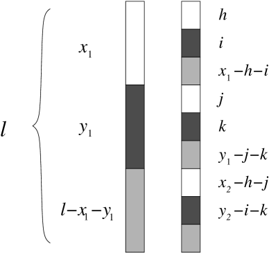
Figure 5: Illustration of the null model for interstrand spatial motifs when $X\neq Y$. White represents $X$ residues, black $Y$ residues, and grey “neither” residues (i.e. neither X nor Y). $X\mbox{-}Y$ motifs are represented by the $i$ residue pairs in which there is an $X$ residue in the first strand and a $Y$ residue in the second, and by the $j$ residue pairs in which there is a $Y$ residue in the first strand and an $X$ residue in the second.

The marginal probability $\mathbb{P}_{X,Y}(m)$ that there are a total of $i+j=m$ $X$-$Y$ contacts in the random model, namely, the pairings where a residue of type $X$ in the first strand is paired with a residue of type $Y$ in the second strand, summed with the pairings in which a residue of type $Y$ in the first strand is paired with a residue of type $X$ in the second strand is:

$$\mathbb{P}_{X,Y}(m)=\sum_{h=0}^{x_{1}}\sum_{i=0}^{x_{1}-h}\sum_{k=0}^{\begin{subarray}{c}y_{1}-\\ (m-i)\end{subarray}}{\mathbb{P}(h,i,m-i,k)},$$

where $h$ is the number of matched $X$-$X$ contacts, $i$ the number of matched $X$-$Y$ contacts, $m-i$ the number of matched $Y$-$X$ contacts($j$ in Figure 5), and $k$ the number of matched $Y$-$Y$ contacts. The remaining contacts involving residues of type “neither” will then automatically be assigned, since all matches involving $X$ and $Y$ have been accounted for. There are $x_{1}$ possible values for $h$, one for each residue of type $X$ on strand 1; $x_{1}-h$ possible values for $i$, once $h$ has been determined; and $y_{1}-j=y-(m-i)$ possible values for $k$, once $i$ has been determined. The $i$ number of $X$-$Y$ contacts plus the $m-i$ number of $Y$-$X$ contacts will sum to the $m$ number of contacts desired. This closed-form formula allows us to calculate analytically the two-tailed $p$-value for this null model of $f^{\prime}(X,Y)$ number of observed $X$-$Y$ contacts using formulae similar to Equations (3) and (4).

Confounding between single-body propensity and interstrand two-body propensity. Because single-body propensities can vary significantly, it is possible that differences in two-body propensities may simply be reflections of differences in single-body propensities, e.g. two polar residues might have high strong H-bond pairwise propensities simply because both residues have an independent preference for the same side of the TM barrel (internal-facing), and not because of any direct significant propensity between the two. This artifact can be eliminated by dividing each strand into two “substrands,” each of which contains only residues facing the same direction. This correction is automatic for strong H-bonds and non-H-bonded interactions, as all of the residues participating in each of these interactions in a single strand pair face the same direction (e.g. the residues in a particular strand pair participating in a strong H-bond must either all be internal or all be external). For weak H-bond interactions, in which one residue is internal and one is external, each strand pair must be divided into two substrand pairs: one pair in which the first substrand is internal and the second is external, and another pair in which the first substrand is external and the second is internal. In this way, the often dominating effects of single-residue orientation are removed from two-body propensity calculation. Results reported in Tables 2 and 3 are obtained after these corrections. For the analysis performed on the soluble $\beta$-sheet dataset, there is no strong distinction between internal and external residues, since only some of the proteins are closed barrels. Thus, no correction was used for weak H-bonds.

Pairwise propensities for a reduced alphabet.

To obtain an objective reduced alphabet of amino acids for studying membrane $\beta$-barrel proteins, we cluster amino acids by their location preference and strand pairing propensities. We represent each amino acid as a vector and use hierarchical clustering to define residue groups. Each vector consists of 68 $z$-scores: one for each of the 20 pairwise contact propensities including the residue for each of the 3 interaction types (strong H-bonds, non-H-bonded interactions, and weak H-bonds), and one for each single-body regional propensity of the residue in each of the 8 regions. The $z$-scores for pairwise propensities are calculated as

$$z(X,Y)=\frac{f(X,Y)-\mathbb{E}[f^{\prime}(X,Y)]}{\sqrt{\operatorname{var}{[f^{\prime}(X,Y)]}}},$$ (5)

and the $z$-scores for single-body propensities are calculated as

$$z(X|r)=\frac{f(X|r)-\mathbb{E}[f^{\prime}(X|r)]}{\sqrt{\operatorname{var}{[f^{\prime}(X|r)]}}}.$$

We use hierarchical clustering by average linkage with a Euclidean distance function to obtain the clustering shown in Figure 3. We place the distance threshold so an alphabet of 5 residues is formed.

Strand register prediction.

Our algorithm consists of two steps, the prediction of exact strand starts and the prediction of strand register. We use two sequence models for these two tasks, namely, a 16-residue single strand model and a 9-residue TM strand pair model (Figure 6). The regional designations in the 16-residue canonical strand model are based on known physical attributes of TM $\beta$-strands: an average length of 9-10 residues in the headgroup and core regions, and an alternating internal-external pattern. The size of each region (the cap regions, headgroup regions, and core region) is determined by dividing the total number of residues in a particular region by the number of strands in the dataset. We have 4 residues for the extracellular cap region, 3 for the periplasmic cap region, 2 each for the two headgroup regions, and 5 for the core region.

The 9-residue strand pair model is derived from the canonical 16-residue models for two adjacent strands. These 9 residues are those designated to be in the transmembrane region, i.e., in the headgroup or core regions. We exclude the 7 cap residues because the cap regions do not contribute to strand pairing. We also incorporate the physical properties of the 3 types of strand interactions in the model: The strong H-bond and non-H-bonded interactions must alternate, and the weak H-bonds must extend one residue in the N-C direction. Due to chirality constraints in antiparallel $\beta$-sheets (i.e. all amino acids in biological proteins are L-amino acids), the backbone H-bonding pattern is fixed once the N-C direction of the strands and the internal-external pattern are determined by step 1. We describe steps 1 and 2 in more detail:

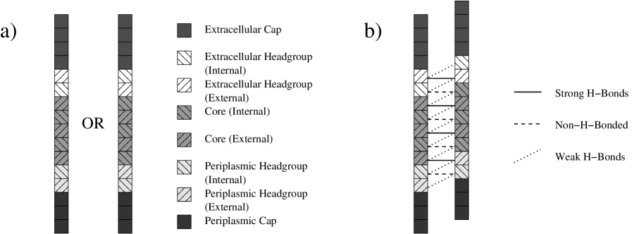
Figure 6: Illustrations of the models for the strand register prediction algorithm. a) 16-residue TM $\beta$-strand model. Two models are scored for each window with different internal-external designations (hatch marks). b) 9-residue strand pair model. The example shown has a strand shear of +1. One strand is shifted up or down against the other (fixed) strand to score different strand shears.

• Predict exact starts. For a 16-residue window fitted to our strand model (Figure 6a), we calculate the single strand energy $E(s;i)$ in $kT$ units for strand $i$:

  $$E(s;i)=-\sum_{k=1}^{16}\ln P(k;i,s),$$

  where $s$ is the displacement of the window position and $P(k;i,s)$ is the single body propensity for the $k$-th residue in this window of strand $i$, where the residues are alternatively assigned as internal and external. We calculate the energy score for a total of 11 possible windows: the window starting at the given approximated strand start $s=0$ (either provided beforehand or calculated by a strand predictor), and all windows 5 residues up ($s\leq+5$) or down ($s\geq-5$) in the amino acid sequence. Because there are two possibilities for the internal-external pattern of TM residues in our model, we calculated strand energy scores for both possibilities for each window. We take the window with the lowest energy as the exact strand start that we use in step 2. The prediction also identifies which residues are internal and which are external.

• Predict strand register. After excluding the 7 cap residues, we fit the 9-residue windows for two adjacent strands to the strand pair model (Figure 6b), and calculate the strand pairing energy $E(s;i,i+1)$ in $kT$ units for the strand pair $(i,i+1)$ with strand shear $s$ as

  $$\begin{split}E(s;i,i+1)=&-\sum{\ln P_{SHB}(k;i,i+1,s)}-\sum{\ln P_{NB}(k;i,i+1,s)}\\ &-\sum{\ln P_{WHB}(k;i,i+1,s)}+\alpha|\frac{N+2}{N}-s|.\end{split}$$

  Here $i$ and $i+1$ are the labels of the two adjacent strands, $P(k;i,i+1,s)$ is the propensity of pairing between the $k$-th residues in strand $i$ and strand $i+1$, and the strand shear $s$ is the residue displacement between the starts of the two strands. The first 3 terms refer to each of the 3 interaction types: strong H-bonds (SHB), non-H-bonded interactions (NB), and weak H-bonds (WHB). The last term represents a penalty to the score when the strand shear $s$ deviates from the average strand shear, approximated as the average shearing number $N+2$ of known TM $\beta$-barrels divided by the number of strands $N$. $\alpha$ is a coefficient determined computationally. We find that $\alpha=2$ works well.

  We calculate the strand pairing score for a total of 11 possible windows by sliding one strand in a pair against the other strand: the windows with a strand shear of $s=-4$ residues up to a strand shear of $s=+6$. We also exclude strand shears that place internal residues next to external residues, as this would violate the H-bonding patterns of $\beta$-sheets. This reduces the search space by half. The strand shear $s$ with the lowest strand pairing energy is taken as the true strand register.

To approximate the strand starts of the $\beta$-barrel membrane proteins in our dataset, we use the hidden Markov model predictor of Bigelow et al. [7], one of the most successful predictors for strand starts. This predictor uses only the amino acid sequence as input, and outputs a designation for each residue from a list of 4 possibilities: “up-strand” (referring to an odd-numbered strand), “down-strand” (even-numbered strand), loop between an up- and down-strand, and loop between a down- and up-strand. This predictor will therefore also predict the number of strands in the protein ab initio. We use the first instances of the up- and down-strand designations for each strand as approximate strand starts.

We exclude from our prediction analysis two proteins in our dataset (6 strand pairs) for which the strand start predictor failed: TolC and $\alpha$-HL. For TolC, the predictor did not detect any TM strands. For $\alpha$-HL, the predictor detected far too many strands (8 instead of the actual 2 strands). For the remaining 17 of the 19 proteins, the hidden Markov model correctly predicted 252 of the 256 strands, with only 4 false positives. The false positive strands were all short (7 residues) and had irregular composition. Our register prediction was also incorrect for all strand pairs involving these 4 false positives. We apply our prediction to the 17 $\beta$-barrel membrane proteins in leave-one-out fashion: we calculate single and pairwise propensities using 16 of the proteins, and use them to predict strand registers in the 17th protein. Since the pairwise propensities are derived from a very small dataset, we introduce a pseudocount of 1 to the observed and expected numbers of each pair when calculating propensities.

References

- [1] M. Montoya, E. Gouaux, -barrel membrane protein folding and structure viewed through the lens of -hemolysin, Biochim Biophys Acta. 1609 (2003) 19–27.
- [2] L. K. Tamm, A. Arora, J. H. Kleinschmidt, Structure and assembly of -barrel membrane proteins, J Biol Chem. 276 (2001) 32399–32402.
- [3] W. C. Wimley, The versatile -barrel membrane protein, Curr Opin Struct Biol. 13 (2003) 404–411.
- [4] L. Song, M. R. Hobaugh, C. Shustak, S. Cheley, H. Bayley, J. E. Gouaux, Structure of staphylococcal -hemolysin, a heptameric transmembrane pore, Science. 274 (1996) 1859–1866.
- [5] S. Nassi, R. J. Collier, A. Finkelstein, PA63 channel of anthrax toxin: an extended -barrel, Biochemistry. 41 (2002) 1445–1450.
- [6] R. Koebnik, K. P. Locher, P. Van Gelder, Structure and function of bacterial outer membrane proteins: barrels in a nutshell, Mol Microbiol. 37 (2000) 239–253.
- [7] H. R. Bigelow, D. S. Petrey, J. Liu, D. Przybylski, B. Rost, Predicting transmembrane -barrels in proteomes, Nucleic Acids Res. 32 (2004) 2566–2577.
- [8] P. L. Martelli, P. Fariselli, A. Krogh, R. Casadio, A sequence-profile-based HMM for predicting and discriminating barrel membrane proteins, Bioinformatics. 18 Suppl 1 (2002) S46–S53.
- [9] M. M. Gromiha, S. Ahmad, M. Suwa, Neural network-based prediction of transmembrane -strand segments in outer membrane proteins, J Comput Chem. 25 (2004) 762–767.
- [10] G. E. Schulz, -barrel membrane proteins, Curr Opin Struct Biol. 10 (2000) 443–447.
- [11] G. E. Schulz, The structure of bacterial outer membrane proteins, Biochim Biophys Acta. 1565 (2002) 308–317.
- [12] L. K. Tamm, H. Hong, B. Liang, Folding and assembly of -barrel membrane proteins, Biochim Biophys Acta. 1666 (2004) 250–263.
- [13] K. Seshadri, R. Garemyr, E. Wallin, G. von Heijne, A. Elofsson, Architecture of -barrel membrane proteins: analysis of trimeric porins, Protein Sci. 7 (1998) 2026–2032.
- [14] W. C. Wimley, Toward genomic identification of -barrel membrane proteins: composition and architecture of known structures, Protein Sci. 11 (2002) 301–312.
- [15] M. B. Ulmschneider, M. S. Sansom, Amino acid distributions in integral membrane protein structures, Biochim Biophys Acta. 1512 (2001) 1–14.
- [16] M. M. Gromiha, M. Suwa, Variation of amino acid properties in all- globular and outer membrane protein structures, Int J Biol Macromol. 32 (2003) 93–98.
- [17] A. K. Chamberlain, J. U. Bowie, Asymmetric amino acid compositions of transmembrane -strands, Protein Sci. 13 (2004) 2270–2274.
- [18] M. A. Wouters, P. M. Curmi, An analysis of side chain interactions and pair correlations within antiparallel -sheets: the differences between backbone hydrogen-bonded and non-hydrogen-bonded residue pairs, Proteins. 22 (1995) 119–131.
- [19] R. E. Steward, J. M. Thornton, Prediction of strand pairing in antiparallel and parallel -sheets using information theory, Proteins. 48 (2002) 178–191.
- [20] J. S. Merkel, L. Regan, Aromatic rescue of glycine in sheets, Fold Des. 3 (1998) 449–455.
- [21] E. G. Hutchinson, R. B. Sessions, J. M. Thornton, D. N. Woolfson, Determinants of strand register in antiparallel -sheets of proteins, Protein Sci. 7 (1998) 2287–2300.
- [22] E. Granseth, G. von Heijne, A. Elofsson, A study of the membrane-water interface region of membrane proteins., J Mol Biol. 346 (2005) 377–385.
- [23] L. Adamian, J. Liang, Helix-helix packing and interfacial pairwise interactions of residues in membrane proteins, J Mol Biol. 311 (2001) 891–907.
- [24] G. von Heijne, Control of topology and mode of assembly of a polytopic membrane protein by positively charged residues, Nature. 341 (1989) 456–458.
- [25] A. K. Chamberlain, Y. Lee, S. Kim, J. U. Bowie, Snorkeling preferences foster an amino acid composition bias in transmembrane helices, J Mol Biol. 339 (2004) 471–479.
- [26] C. M. Wilmot, J. M. Thornton, Analysis and prediction of the different types of -turn in proteins, J Mol Biol. 203 (1988) 221–232.
- [27] G. E. Schulz, The structures of general porins, in: R. Benz (Ed.), Bacterial and Eukaryotic Porins, WILEY-VCH, 2004, pp. 25–40.
- [28] L. Adamian, J. Liang, Interhelical hydrogen bonds and spatial motifs in membrane proteins: polar clamps and serine zippers, Proteins. 47 (2002) 209–218.
- [29] L. Adamian, R. Jackups, T. A. Binkowski, J. Liang, Higher-order interhelical spatial interactions in membrane proteins, J Mol Biol. 327 (2003) 251–272.
- [30] M. Eilers, A. B. Patel, W. Liu, S. O. Smith, Comparison of helix interactions in membrane and soluble -bundle proteins, Biophys J. 82 (2002) 2720–2736.
- [31] W. Liu, M. Eilers, A. B. Patel, S. O. Smith, Helix packing moments reveal diversity and conservation in membrane protein structure, J Mol Biol. 337 (2004) 713–729.
- [32] M. Gimpelev, L. R. Forrest, D. Murray, B. Honig, Helical packing patterns in membrane and soluble proteins, Biophys J. 87 (2004) 4075–4086.
- [33] B. K. Ho, P. M. Curmi, Twist and shear in -sheets and -ribbons, J Mol Biol. 317 (2002) 291–308.
- [34] A. Senes, I. Ubarretxena-Belandia, D. M. Engelman, The C–HO hydrogen bond: a determinant of stability and specificity in transmembrane helix interactions, Proc Natl Acad Sci U S A. 98 (2001) 9056–9061.
- [35] D. S. Riddle, J. V. Santiago, S. T. Bray-Hall, N. Doshi, V. P. Grantcharova, Q. Yi, D. Baker, Functional rapidly folding proteins from simplified amino acid sequences, Nat Struct Biol. 4 (1997) 805–809.
- [36] L. R. Murphy, A. Wallqvist, R. M. Levy, Simplified amino acid alphabets for protein fold recognition and implications for folding, Protein Eng. 13 (2000) 149–152.
- [37] X. Li, C. Hu, J. Liang, Simplicial edge representation of protein structures and alpha contact potential with confidence measure, Proteins. 53 (2003) 792–805.
- [38] I. N. Shindyalov, P. E. Bourne, Protein structure alignment by incremental combinatorial extension (CE) of the optimal path., Protein Eng. 9 (1998) 739–747.
- [39] S. H. White, W. C. Wimley, Membrane protein folding and stability: physical principles, Annu Rev Biophys Biomol Struct. 28 (1999) 319–365.
- [40] A. K. Chamberlain, J. U. Bowie, Analysis of side-chain rotamers in transmembrane proteins, Biophys J. 87 (2004) 3460–3469.
- [41] T. Nakae, Outer-membrane permeability of bacteria, Crit Rev Microbiol. 13 (1986) 1–62.
- [42] H. de Cock, J. Tommassen, Lipopolysaccharides and divalent cations are involved in the formation of an assembly-competent intermediate of outer-membrane protein PhoE of E. coli, EMBO J. 15 (1996) 5567–5573.
- [43] A. D. Ferguson, E. Hofmann, J. W. Coulton, K. Diederichs, W. Welte, Siderophore-mediated iron transport: crystal structure of FhuA with bound lipopolysaccharide, Science. 282 (1998) 2215–2220.
- [44] H. Nikaido, Molecular basis of bacterial outer membrane permeability revisited, Microbiol Mol Biol Rev. 67 (2003) 593–656.
- [45] M. Ramakrishnan, C. L. Pocanschi, J. H. Kleinschmidt, D. Marsh, Association of spin-labeled lipids with -barrel proteins from the outer membrane of Escherichia coli, Biochemistry. 43 (2004) 11630–11636.
- [46] W. van Klompenburg, I. Nilsson, G. von Heijne, B. de Kruijff, Anionic phospholipids are determinants of membrane protein topology, EMBO J. 16 (1997) 4261–4266.
- [47] S. H. White, G. von Heijne, The machinery of membrane protein assembly, Curr Opin Struct Biol. 14 (2004) 397–404.
- [48] J. H. Kleinschmidt, L. K. Tamm, Time-resolved distance determination by tryptophan fluorescence quenching: probing intermediates in membrane protein folding, Biochemistry. 38 (1999) 4996–5005.
- [49] T. R. Weikl, K. A. Dill, Folding kinetics of two-state proteins: effect of circularization, permutation, and crosslinks., J Mol Biol. 332 (2003) 953–963.
- [50] W. Kabsch, C. Sander, Dictionary of protein secondary structure: pattern recognition of hydrogen-bonded and geometrical features, Biopolymers. 22 (1983) 2577–2637.
- [51] A. Pautsch, G. E. Schulz, Structure of the outer membrane protein A transmembrane domain, Nat Struct Biol. 5 (1998) 1013–1017.
- [52] J. Vogt, G. E. Schulz, The structure of the outer membrane protein OmpX from Escherichia coli reveals possible mechanisms of virulence, Structure Fold Des. 7 (1999) 1301–1309.
- [53] L. Vandeputte-Rutten, M. P. Bos, J. Tommassen, P. Gros, Crystal structure of Neisserial surface protein A (NspA), a conserved outer membrane protein with vaccine potential, J Biol Chem. 278 (2003) 24825–24830.
- [54] S. M. Prince, M. Achtman, J. P. Derrick, Crystal structure of the OpcA integral membrane adhesin from Neisseria meningitidis, Proc Natl Acad Sci U S A. 99 (2002) 3417–3421.
- [55] L. Vandeputte-Rutten, R. A. Kramer, J. Kroon, N. Dekker, M. R. Egmond, P. Gros, Crystal structure of the outer membrane protease OmpT from Escherichia coli suggests a novel catalytic site, EMBO J. 20 (2001) 5033–5039.
- [56] H. J. Snijder, I. Ubarretxena-Belandia, M. Blaauw, K. H. Kalk, H. M. Verheij, M. R. Egmond, N. Dekker, B. W. Dijkstra, Structural evidence for dimerization-regulated activation of an integral membrane phospholipase, Nature. 401 (1999) 717–721.
- [57] C. J. Oomen, P. Van Ulsen, P. Van Gelder, M. Feijen, J. Tommassen, P. Gros, Structure of the translocator domain of a bacterial autotransporter, EMBO J. 23 (2004) 1257–1266.
- [58] M. S. Weiss, G. E. Schulz, Structure of porin refined at 1.8 Å resolution, J Mol Biol. 227 (1992) 493–509.
- [59] A. Kreusch, G. E. Schulz, Refined structure of the porin from Rhodopseudomonas blastica. Comparison with the porin from Rhodobacter capsulatus, J Mol Biol. 243 (1994) 891–905.
- [60] S. Cowan, R. M. Garavito, J. N. Jansonius, J. A. Jenkins, R. Karlsson, N. Konig, E. F. Pai, R. A. Pauptit, P. J. Rizkallah, J. P. Rosenbusch, et al., The structure of OmpF porin in a tetragonal crystal form, Structure. 3 (1995) 1041–1050.
- [61] K. Zeth, K. Diederichs, W. Welte, H. Engelhardt, Crystal structure of Omp32, the anion-selective porin from Comamonas acidovorans, in complex with a periplasmic peptide at 2.1 Å resolution, Structure Fold Des. 8 (2000) 981–992.
- [62] J. E. Meyer, M. Hofnung, G. E. Schulz, Structure of maltoporin from Salmonella typhimurium ligated with a nitrophenyl-maltotrioside, J Mol Biol. 266 (1997) 761–775.
- [63] D. Forst, W. Welte, T. Wacker, K. Diederichs, Structure of the sucrose-specific porin ScrY from Salmonella typhimurium and its complex with sucrose, Nat Struct Biol. 5 (1998) 37–46.
- [64] S. K. Buchanan, B. S. Smith, L. Venkatramani, D. Xia, L. Esser, M. Palnitkar, R. Chakraborty, D. van der Helm, J. Deisenhofer, Crystal structure of the outer membrane active transporter FepA from Escherichia coli, Nat Struct Biol. 6 (1999) 56–63.
- [65] A. D. Ferguson, R. Chakraborty, B. S. Smith, L. Esser, D. Van Der Helm, J. Deisenhofer, Structural basis of gating by the outer membrane transporter FecA, Science. 295 (2002) 1715–1719.
- [66] D. P. Chimento, A. K. Mohanty, R. J. Kadner, M. C. Wiener, Substrate-induced transmembrane signaling in the cobalamin transporter BtuB, Nat Struct Biol. 10 (2003) 394–401.
- [67] V. Koronakis, A. J. Sharff, E. Koronakis, B. Luisi, C. Hughes, Crystal structure of the bacterial membrane protein TolC central to multidrug efflux and protein export, Nature. 405 (2000) 914–919.