Time-dependent perturbation theory for vibrational energy relaxation and dephasing in peptides and proteins

Abstract

Without invoking the Markov approximation, we derive formulas for vibrational energy relaxation (VER) and dephasing for an anharmonic system oscillator using a time-dependent perturbation theory. The system-bath Hamiltonian contains more than the third order coupling terms since we take a normal mode picture as a zeroth order approximation. When we invoke the Markov approximation, our theory reduces to the Maradudin-Fein formula which is used to describe VER properties of glass and proteins. When the system anharmonicity and the renormalization effect due to the environment vanishes, our formulas reduce to those derived by Mikami and Okazaki invoking the path-integral influence functional method [J. Chem. Phys. 121, 10052 (2004)]. We apply our formulas to VER of the amide I mode of a small amino-acide like molecule, $N$-methylacetamide, in heavy water.

I Introduction

Vibrational energy relaxation (VER) and dephasing are fundamental properties of molecular dynamics, energy transfer, and reactivity. Many experimental and theoretical studies have explored these fundamental processes in gas phase, the liquid state, and in glasses and biomolecular systems FS05 . Though our methodology can be applied to any molecular system, we are primarily interested in addressing VER and dephasing in peptides or proteins. While recent advanced experimental techniques using absorption spectra or time-resolved spectra can deduce the structure and dynamics of such a peptide or protein system, theoretical approaches are needed to clarify the mechanisms of VER and dephasing underlying the experimental data.

The most standard approach to this problem is through the perturbation theory of quantum mechanics as initiated by Oxtoby Oxtoby . Recently Hynes’s group Hynes and Skinner’s group Skinner thoroughly studied the VER and dephasing properties of water (their target mode was the OH bond of HOD in heavy water) using this strategy. This approach is applicable to peptides or proteins as was first illustrated by Straub and coworkers Straub . Derived from this strategy is the use of the Maradudin-Fein formula (or its equivalent), which was pursued by Leitner Leitner05 and Straub and coworkers FBS05a . This formula requires the normal modes of the system and the cubic anharmonic coefficients between the normal modes. This methodology can provide a reasonable account of VER properties of peptides or proteins, but there are several deficiencies: the most serious one is that it assumes the Markov properties of the system, so it cannot describe the short time dynamics FBS05b . Another problem is the determination of the “lifetime” width parameter FS05 ; FBS05a ; FBS05b . We also want to describe the dephasing properties of the system, crucial to the interpretation of the experimental results; it cannot be directly described by the MF formula (but see Leitner02 ).

To meet these goals, we derive the formulas for VER and dephasing without assuming the Markov properties, i.e., without taking an infinite-time limit. As a result, we can avoid the annoying “width parameter” problem inherent to the MF approach. In this sense, Mikami and Okazaki MO04 took a similar path using the path-integral influence functional theory. We use a simple time-dependent perturbation theory of quantum mechanics, and derive the VER and dephasing formulas more easily. We find there is a difference between our formulas and theirs in terms of renormalization of the system Hamiltonian. Another difference is that our system oscillator is taken to be a cubic anharmonic oscillator, whereas their mode is a harmonic oscillator. This can affect the result when the formulas are applied to real systems with strong anharmonicity.

This paper is organized as follows: In Sec. II, we derive the VER and dephasing formulas for an anharmonic oscillator (mode) without assuming the Markov properties. In Sec. III, we apply our formulas to the amide I mode of $N$-methylacetamide in heavy water, and discuss the numerical results and the limitations of our strategy. In Sec. IV, we summarize the paper. Several system parameters and coefficients in our formulas are defined in the Appendix.

II Derivation of the formulas for VER and dephasing

II.1 System, Bath, and Coupling

We take our Hamiltonian of a solvated peptide or protein to be

$${\cal H} = {\cal H}_{0}+{\cal V}={\cal H}_{S}+{\cal H}_{B}+{\cal V}={\cal H}_{S}^{(0)}+{\cal H}_{f}+{\cal H}_{B}+{\cal V},$$ (1)

$${\cal V} = -q_{S}({\cal F}-\langle{\cal F}\rangle)+q_{S}^{2}({\cal G}-\langle{\cal G}\rangle)=-q_{S}\delta{\cal F}+q_{S}^{2}\delta{\cal G},$$ (2)

$${\cal H}_{S}^{(0)} = \frac{p_{S}^{2}}{2}+\frac{\omega_{S}^{2}}{2}q_{S}^{2}-q_{S}\langle{\cal F}\rangle+q_{S}^{2}\langle{\cal G}\rangle=\frac{p_{S}^{2}}{2}+\frac{\bar{\omega}_{S}^{2}}{2}\bar{q}_{S}^{2}-\frac{\langle{\cal F}\rangle^{2}}{2\bar{\omega}_{S}^{2}},$$ (3)

$${\cal H}_{f} = \frac{f}{6}\bar{q}_{S}^{3},$$ (4)

$${\cal H}_{B} = \sum_{\alpha}\left(\frac{p_{\alpha}^{2}}{2}+\frac{\omega_{\alpha}^{2}}{2}q_{\alpha}^{2}\right),$$ (5)

where

$$\bar{\omega}_{S} = \omega_{S}\sqrt{1+\frac{2\langle{\cal G}\rangle}{\omega_{S}^{2}}},$$ (6)

$$\bar{q}_{S} = q_{S}-\frac{\langle{\cal F}\rangle}{\bar{\omega}_{S}^{2}}=q_{S}-b.$$ (7)

${\cal H}_{S}={\cal H}_{S}^{(0)}+{\cal H}_{f}$ is the renormalized system Hamiltonian representing a vibrational mode $q_{S}$ with cubic anharmonicity $f$, ${\cal H}_{B}$ the bath Hamiltonian representing solvent or environmental degrees of freedom with harmonic frequencies $\omega_{\alpha}$, and ${\cal V}$ the interaction Hamiltonian describing the coupling between the system and the bath. We have assumed that the interation can be Taylor expanded, and we have only included up to the second order in $q_{S}$. Note that we need to renormalize the system to assure that $\langle{\cal V}\rangle=0$ where the bracket denotes the bath average throughout this paper. (For the definition of $\delta{\cal F}$ and $\delta{\cal G}$, see Appendix A.) This is automatically satisfied in the case of bilinear coupling like the Caldeira-Leggett-Zwanzig model Weiss , but this is not usually the case. The system variable becomes ${\bar{q}}_{S}$ instead of $q_{S}$, and the system frequency does ${\bar{\omega}}_{S}$ instead of $\omega_{S}$. This is similar to previous treatments of the system-bath interaction in the literature Skinner ; XYK02 .

II.2 Perturbation theory for VER and dephasing

Starting from the interaction picture of the von Neumann equation, we can expand the density operator for the full system as

$$\tilde{\rho}(t) = \rho(0)+\frac{1}{i\hbar}\int_{0}^{t}dt^{\prime}[\tilde{\cal V}(t^{\prime}),\tilde{\rho}(t^{\prime})]$$ (8)

$$= \rho(0)+\frac{1}{i\hbar}\int_{0}^{t}dt^{\prime}[\tilde{\cal V}(t^{\prime}),\rho(0)]$$

$$+\frac{1}{(i\hbar)^{2}}\int_{0}^{t}dt^{\prime}\int_{0}^{t^{\prime}}dt^{\prime\prime}[\tilde{\cal V}(t^{\prime}),[\tilde{\cal V}(t^{\prime\prime}),\rho(0)]]+\cdots$$

where

$$\tilde{\rho}(t)\equiv e^{i{\cal H}_{0}t/\hbar}\rho(t)e^{-i{\cal H}_{0}t/\hbar},\hskip 28.45274pt\tilde{\cal V}(t)\equiv e^{i{\cal H}_{0}t/\hbar}{\cal V}e^{-i{\cal H}_{0}t/\hbar}.$$ (9)

The reduced density matrix for the system oscillator is introduced as

$$(\rho_{S})_{mn}(t) \equiv {\rm Tr}\{P_{mn}\rho(t)\}={\rm Tr}\{P_{mn}e^{-i{\cal H}_{0}t/\hbar}\tilde{\rho}(t)e^{i{\cal H}_{0}t/\hbar}\},$$ (10)

$$P_{mn} \equiv |n\rangle\langle m|\otimes 1_{B},$$ (11)

$$\rho(0) = \rho_{S}\otimes\rho_{B}=\sum_{k,l}(\rho_{S})_{kl}|k\rangle\langle l|\otimes e^{-\beta{\cal H}_{B}}/Z_{B},$$ (12)

$$Z_{B} = {\rm Tr}_{B}\{e^{-\beta{\cal H}_{B}}\},$$ (13)

where the initial state is assumed to be a direct product state of $\rho_{S}$ and $\rho_{B}=e^{-\beta{\cal H}_{B}}/Z_{B}$, i.e., we have assumed that the bath is in thermal equilibrium. Here $|k\rangle$ is the vibrational eigenstate for the system Hamiltonian ${\cal H}_{S}$, i.e., ${\cal H}_{S}|k\rangle=E_{k}|k\rangle$. If we assume that ${\cal H}_{f}$ is small, we can calculate $|k\rangle$ and $E_{k}$ using the time-independent perturbation theory as shown in Appendix A.

We note that

$$(\rho_{S})_{mn}(t)={\rm Tr}\{P_{mn}e^{-i{\cal H}_{0}t/\hbar}\tilde{\rho}(t)e^{i{\cal H}_{0}t/\hbar}\}={\rm Tr}_{B}\{\tilde{\rho}_{mn}(t)\}e^{-i\omega_{mn}t}.$$ (14)

The lowest (second) order result for the density matrix is

$$(\rho_{S})_{mn}(t) \simeq (\rho_{S})^{(0)}_{mn}(t)+(\rho_{S})^{(1)}_{mn}(t)+(\rho_{S})^{(2)}_{mn}(t)+\cdots,$$ (15)

$$(\rho_{S})^{(0)}_{mn}(t) = {\rm Tr}_{B}\{\tilde{\rho}_{mn}(0)\}e^{-i\omega_{mn}t}=(\rho_{S})_{mn}e^{-i\omega_{mn}t},$$ (16)

$$(\rho_{S})^{(1)}_{mn}(t) = \frac{1}{i\hbar}\int^{t}_{0}dt^{\prime}{\rm Tr}_{B}\{\langle m|[\tilde{\cal V}(t^{\prime}),\rho(0)]|n\rangle\}e^{-i\omega_{mn}t}$$ (17)

$$= \frac{1}{i\hbar}\int^{t}_{0}dt^{\prime}\sum_{k}\left\{\langle\tilde{\cal V}_{mk}(t^{\prime})\rangle e^{i\omega_{mk}t^{\prime}}(\rho_{S})_{kn}-\langle\tilde{\cal V}_{kn}(t^{\prime})\rangle e^{i\omega_{kn}t^{\prime}}(\rho_{S})_{mk}\right\}e^{-i\omega_{mn}t},$$

$$(\rho_{S})^{(2)}_{mn}(t) = \frac{1}{(i\hbar)^{2}}\int^{t}_{0}dt^{\prime}\int^{t^{\prime}}_{0}dt^{\prime\prime}{\rm Tr}_{B}\{\langle m|[\tilde{\cal V}(t^{\prime}),[\tilde{\cal V}(t^{\prime\prime}),\rho(0)]]|n\rangle\}e^{-i\omega_{mn}t}$$ (18)

$$= \frac{1}{(i\hbar)^{2}}\int_{0}^{t}dt^{\prime}\int_{0}^{t^{\prime}}dt^{\prime\prime}\sum_{k,l}\left\{\langle\tilde{\cal V}_{mk}(t^{\prime})\tilde{\cal V}_{kl}(t^{\prime\prime})\rangle(\rho_{S})_{ln}e^{i(\omega_{mk}t^{\prime}+\omega_{kl}t^{\prime\prime})}\right\}e^{-i\omega_{mn}t}$$

$$+ \frac{1}{(i\hbar)^{2}}\int_{0}^{t}dt^{\prime}\int_{0}^{t^{\prime}}dt^{\prime\prime}\sum_{k,l}\left\{\langle\tilde{\cal V}_{kl}(t^{\prime\prime})\tilde{\cal V}_{ln}(t^{\prime})\rangle(\rho_{S})_{mk}e^{i(\omega_{kl}t^{\prime\prime}+\omega_{ln}t^{\prime})}\right\}e^{-i\omega_{mn}t}$$

$$- \frac{1}{(i\hbar)^{2}}\int_{0}^{t}dt^{\prime}\int_{0}^{t^{\prime}}dt^{\prime\prime}\sum_{k,l}\left\{\langle\tilde{\cal V}_{ln}(t^{\prime\prime})\tilde{\cal V}_{mk}(t^{\prime})\rangle(\rho_{S})_{kl}e^{i(\omega_{mk}t^{\prime}+\omega_{ln}t^{\prime\prime})}\right\}e^{-i\omega_{mn}t}$$

$$- \frac{1}{(i\hbar)^{2}}\int_{0}^{t}dt^{\prime}\int_{0}^{t^{\prime}}dt^{\prime\prime}\sum_{k,l}\left\{\langle\tilde{\cal V}_{ln}(t^{\prime})\tilde{\cal V}_{mk}(t^{\prime\prime})\rangle(\rho_{S})_{kl}e^{i(\omega_{mk}t^{\prime\prime}+\omega_{ln}t^{\prime})}\right\}e^{-i\omega_{mn}t}$$

where

$$\langle\tilde{\cal V}_{kl}(t)\tilde{\cal V}_{mn}(t^{\prime})\rangle \equiv {\rm Tr}_{B}\{\rho_{B}\tilde{\cal V}_{kl}(t)\tilde{\cal V}_{mn}(t^{\prime})\},$$ (19)

$$\tilde{\cal V}_{kl}(t) = \langle k|\tilde{\cal V}(t)|l\rangle=\langle k|e^{i{\cal H}_{B}t/\hbar}{\cal V}e^{-i{\cal H}_{B}t/\hbar}|l\rangle,$$ (20)

$$\omega_{kl} = (E_{k}-E_{l})/\hbar.$$ (21)

Note that, in the above formulas, the time dependence is only induced by the bath Hamiltonian ${\cal H}_{B}$.

For the matrix elements of the interaction Hamiltonian ${\cal V}$, we have

$$\langle\tilde{\cal V}_{kl}(t)\rangle = -(q_{S})_{kl}\langle\delta{\cal F}(t)\rangle+(q_{S}^{2})_{kl}\langle\delta{\cal G}(t)\rangle,$$ (22)

$$\langle\tilde{\cal V}_{kl}(t)\tilde{\cal V}_{mn}(t^{\prime})\rangle = (q_{S})_{kl}(q_{S})_{mn}\langle\delta{\cal F}(t)\delta{\cal F}(t^{\prime})\rangle+(q_{S}^{2})_{kl}(q_{S}^{2})_{mn}\langle\delta{\cal G}(t)\delta{\cal G}(t^{\prime})\rangle$$ (23)

$$-[(q_{S})_{kl}(q_{S}^{2})_{mn}+(q_{S}^{2})_{kl}(q_{S})_{mn}]\langle\delta{\cal F}(t)\delta{\cal G}(t^{\prime})\rangle$$

where the value of $(q_{S})_{kl}$ and $(q_{S}^{2})_{kl}$ are given in Eqs. (65)-(70) for the case of a cubic oscillator. Since $\langle\delta{\cal F}\rangle=0$ and $\langle\delta{\cal G}\rangle=0$, we have $\langle\tilde{\cal V}_{kl}(t)\rangle=0$ and $(\rho_{S})^{(1)}_{mn}(t)=0$.

II.3 VER formula

We first calculate the diagonal elements of the density matrix $(\rho_{S})_{ii}(t)$ ($i=0,1$) by assuming that the initial state is the first vibrationally excited state: $\rho_{S}=|1\rangle\langle 1|$. This is a typical situation for VER though VER from highly excited states can be considered VFVAMJ04 . The density matrix $(\rho_{S})_{00}(t)$ is written as

$$(\rho_{S})_{00}(t) \simeq \frac{2}{\hbar^{2}}\int_{0}^{t}dt^{\prime}\int_{0}^{t^{\prime}}dt^{\prime\prime}{\rm Re}\left\{\langle\tilde{\cal V}_{10}(t^{\prime})\tilde{\cal V}_{01}(t^{\prime\prime})\rangle e^{i\tilde{\omega}_{S}(t^{\prime}-t^{\prime\prime})}\right\}$$ (24)

where $\tilde{\omega}_{S}$ is the anharmonicity-corrected system frequency given by Eq. (62).

From Eq. (23), we have

$$(\rho_{S})_{00}(t) \simeq \frac{2}{\hbar^{2}}(q_{S})^{2}_{10}\int_{0}^{t}dt^{\prime}\int_{0}^{t^{\prime}}dt^{\prime\prime}{\rm Re}\left\{\langle\delta{\cal F}(t^{\prime}-t^{\prime\prime})\delta{\cal F}(0)\rangle e^{i\tilde{\omega}_{S}(t^{\prime}-t^{\prime\prime})}\right\}$$ (25)

$$+\frac{2}{\hbar^{2}}(q^{2}_{S})^{2}_{10}\int_{0}^{t}dt^{\prime}\int_{0}^{t^{\prime}}dt^{\prime\prime}{\rm Re}\left\{\langle\delta{\cal G}(t^{\prime}-t^{\prime\prime})\delta{\cal G}(0)\rangle e^{i\tilde{\omega}_{S}(t^{\prime}-t^{\prime\prime})}\right\}$$

$$-\frac{4}{\hbar^{2}}(q_{S})_{10}(q^{2}_{S})_{10}\int_{0}^{t}dt^{\prime}\int_{0}^{t^{\prime}}dt^{\prime\prime}{\rm Re}\left\{\langle\delta{\cal F}(t^{\prime}-t^{\prime\prime})\delta{\cal G}(0)\rangle e^{i\tilde{\omega}_{S}(t^{\prime}-t^{\prime\prime})}\right\}.$$

Using the explicit expressions for the correlation functions FBS05a , the final VER formula is obtained as

$$(\rho_{S})_{00}(t) \simeq \frac{2}{\hbar^{2}}\sum_{\alpha,\beta}\left[C_{--}^{\alpha\beta}u_{t}(\tilde{\omega}_{S}-\omega_{\alpha}-\omega_{\beta})+C_{++}^{\alpha\beta}u_{t}(\tilde{\omega}_{S}+\omega_{\alpha}+\omega_{\beta})+C_{+-}^{\alpha\beta}u_{t}(\tilde{\omega}_{S}-\omega_{\alpha}+\omega_{\beta})\right]$$ (26)

$$+\frac{2}{\hbar^{2}}\sum_{\alpha}\left[C^{\alpha}_{-}u_{t}(\tilde{\omega}_{S}-\omega_{\alpha})+C^{\alpha}_{+}u_{t}(\tilde{\omega}_{S}+\omega_{\alpha})\right]$$

where $u_{t}(\Omega)$ is defined as

$$u_{t}(\Omega) = \int_{0}^{t}dt^{\prime}\int_{0}^{t^{\prime}}dt^{\prime\prime}\cos\Omega(t^{\prime}-t^{\prime\prime})=\frac{1-\cos\Omega t}{\Omega^{2}},$$ (27)

$$v_{t}(\Omega) = \int_{0}^{t}dt^{\prime}\int_{0}^{t^{\prime}}dt^{\prime\prime}\sin\Omega(t^{\prime}-t^{\prime\prime})=\frac{\Omega t-\sin\Omega t}{\Omega^{2}},$$ (28)

and $v_{t}(\Omega)$ is defined for later use. The coefficients are defined in Appendix B. Equation (26) is our final formula for VER.

If we take the long time limit of this formula (which is equivalent to the Markov approximation), we obtain a formula for the VER rate

$$k_{0\leftarrow 1} \equiv \left.\frac{d}{dt}(\rho_{S})_{00}(t)\right|_{t\rightarrow\infty}$$ (29)

$$= \frac{2\pi}{\hbar^{2}}\sum_{\alpha,\beta}\left[C_{--}^{\alpha\beta}\delta(\tilde{\omega}_{S}-\omega_{\alpha}-\omega_{\beta})+C_{++}^{\alpha\beta}\delta(\tilde{\omega}_{S}+\omega_{\alpha}+\omega_{\beta})+C_{+-}^{\alpha\beta}\delta(\tilde{\omega}_{S}-\omega_{\alpha}+\omega_{\beta})\right]$$

$$+\frac{2\pi}{\hbar^{2}}\sum_{\alpha}\left[C^{\alpha}_{-}\delta(\tilde{\omega}_{S}-\omega_{\alpha})+C^{\alpha}_{+}\delta(\tilde{\omega}_{S}+\omega_{\alpha})\right]$$

where we have used

$$\left.\frac{d}{dt}u_{t}(\Omega)\right|_{t\rightarrow\infty}=\left.\frac{\sin\Omega t}{\Omega}\right|_{t\rightarrow\infty}=\pi\delta(\Omega).$$ (30)

If $\bar{q}_{S}=q_{S}$ and $\tilde{\omega}_{S}=\omega_{S}$, i.e., $\langle{\cal F}\rangle=\langle{\cal G}\rangle=0$ and $f=0$, we recover the Maradudin-Fein formula FBS05a from Eq. (29). It follows that Eq. (26) is a generalization of the Maradudin-Fein formula, which can describe the time development of a density matrix.

II.4 Dephasing formula

We calculate the off diagonal elements of the density matrix $(\rho_{S})_{10}(t)$ by assuming that the initial state is the superposition state between $|0\rangle$ and $|1\rangle$: $\rho_{S}=(1/2)(|0\rangle\langle 0|+|0\rangle\langle 1|+|1\rangle\langle 0|+|1\rangle\langle 1|)$ MO04 . That is, $(\rho_{S})_{kl}=1/2$ for all $k$ and $l$. This is a simplified situation to consider dephasing in a two-level system. We have

$$(\rho_{S})_{10}(t) = (\rho_{S})^{(0)}_{10}(t)+(\rho_{S})^{(1)}_{10}(t)+(\rho_{S})^{(2)}_{10}(t)+\cdots$$ (31)

$$= \frac{1}{2}e^{-i\tilde{\omega}_{S}t}(1+r^{(1)}(t)+r^{(2)}(t)+\cdots).$$

By the definition of the interaction Hamiltonian (Appendix A), we have $r^{(1)}(t)=0$. The remaining term $r^{(2)}(t)$ is decomposed as

$$r^{(2)}(t) = -r^{(2)}_{FF}(t)-r^{(2)}_{GG}(t)-r^{(2)}_{FG}(t),$$ (32)

$$r^{(2)}_{FF}(t) = \frac{2}{\hbar^{2}}\int_{0}^{t}dt^{\prime}\int_{0}^{t^{\prime}}dt^{\prime\prime}{\rm Re}\{\langle{\cal V}_{10}(t^{\prime}){\cal V}_{01}(t^{\prime\prime})\rangle\}[e^{i\tilde{\omega}_{S}(t^{\prime}-t^{\prime\prime})}-e^{i\tilde{\omega}_{S}(t^{\prime}+t^{\prime\prime})}]$$ (33)

$$= \frac{2}{\hbar^{2}}(q_{S})_{10}^{2}\int_{0}^{t}dt^{\prime}\int_{0}^{t^{\prime}}dt^{\prime\prime}{\rm Re}\{\langle\delta{\cal F}(t^{\prime})\delta{\cal F}(t^{\prime\prime})\rangle\}[e^{i\tilde{\omega}_{S}(t^{\prime}-t^{\prime\prime})}-e^{i\tilde{\omega}_{S}(t^{\prime}+t^{\prime\prime})}]$$

$$+ \frac{2}{\hbar^{2}}(q^{2}_{S})_{10}^{2}\int_{0}^{t}dt^{\prime}\int_{0}^{t^{\prime}}dt^{\prime\prime}{\rm Re}\{\langle\delta{\cal G}(t^{\prime})\delta{\cal G}(t^{\prime\prime})\rangle\}[e^{i\tilde{\omega}_{S}(t^{\prime}-t^{\prime\prime})}-e^{i\tilde{\omega}_{S}(t^{\prime}+t^{\prime\prime})}]$$

$$- \frac{4}{\hbar^{2}}(q_{S})_{10}(q^{2}_{S})_{10}\int_{0}^{t}dt^{\prime}\int_{0}^{t^{\prime}}dt^{\prime\prime}{\rm Re}\{\langle\delta{\cal F}(t^{\prime})\delta{\cal G}(t^{\prime\prime})\rangle\}[e^{i\tilde{\omega}_{S}(t^{\prime}-t^{\prime\prime})}-e^{i\tilde{\omega}_{S}(t^{\prime}+t^{\prime\prime})}],$$

$$r^{(2)}_{GG}(t) = \frac{1}{\hbar^{2}}\int_{0}^{t}dt^{\prime}\int_{0}^{t^{\prime}}dt^{\prime\prime}\{\langle[{\cal V}_{11}(t^{\prime})-{\cal V}_{00}(t^{\prime})]{\cal V}_{11}(t^{\prime\prime})\rangle+\langle{\cal V}_{00}(t^{\prime\prime})[{\cal V}_{00}(t^{\prime})-{\cal V}_{11}(t^{\prime})]\rangle\}$$ (34)

$$= \frac{1}{\hbar^{2}}[(q_{S})_{11}-(q_{S})_{00}]^{2}\int_{0}^{t}dt^{\prime}\int_{0}^{t^{\prime}}dt^{\prime\prime}{\rm Re}\langle\delta{\cal F}(t^{\prime})\delta{\cal F}(t^{\prime\prime})\rangle$$

$$+ \frac{1}{\hbar^{2}}[(q^{2}_{S})_{11}-(q^{2}_{S})_{00}]^{2}\int_{0}^{t}dt^{\prime}\int_{0}^{t^{\prime}}dt^{\prime\prime}{\rm Re}\langle\delta{\cal G}(t^{\prime})\delta{\cal G}(t^{\prime\prime})\rangle$$

$$- \frac{2}{\hbar^{2}}[(q_{S})_{11}-(q_{S})_{00}][(q^{2}_{S})_{11}-(q^{2}_{S})_{00}]\int_{0}^{t}dt^{\prime}\int_{0}^{t^{\prime}}dt^{\prime\prime}{\rm Re}\langle\delta{\cal F}(t^{\prime})\delta{\cal G}(t^{\prime\prime})\rangle$$

$$+ \frac{i}{\hbar^{2}}[(q_{S})^{2}_{11}-(q_{S})^{2}_{00}]\int_{0}^{t}dt^{\prime}\int_{0}^{t^{\prime}}dt^{\prime\prime}{\rm Im}\langle\delta{\cal F}(t^{\prime})\delta{\cal F}(t^{\prime\prime})\rangle$$

$$+ \frac{i}{\hbar^{2}}[(q^{2}_{S})^{2}_{11}-(q^{2}_{S})^{2}_{00}]\int_{0}^{t}dt^{\prime}\int_{0}^{t^{\prime}}dt^{\prime\prime}{\rm Im}\langle\delta{\cal G}(t^{\prime})\delta{\cal G}(t^{\prime\prime})\rangle$$

$$- \frac{2i}{\hbar^{2}}[(q_{S})_{11}(q^{2}_{S})_{11}-(q^{2}_{S})_{00}(q^{2}_{S})_{00}]\int_{0}^{t}dt^{\prime}\int_{0}^{t^{\prime}}dt^{\prime\prime}{\rm Im}\langle\delta{\cal F}(t^{\prime})\delta{\cal G}(t^{\prime\prime})\rangle,$$

$$r^{(2)}_{FG}(t) = \frac{2i}{(i\hbar)^{2}}\int_{0}^{t}dt^{\prime}\int_{0}^{t^{\prime}}dt^{\prime\prime}{\rm Im}\{\langle[{\cal V}_{11}(t^{\prime})-{\cal V}_{00}(t^{\prime})]{\cal V}_{10}(t^{\prime\prime})\rangle\}[e^{i\tilde{\omega}_{S}t^{\prime}}-e^{i\tilde{\omega}_{S}t^{\prime\prime}}]$$ (35)

$$= \frac{2i}{(i\hbar)^{2}}[(q_{S})_{11}-(q_{S})_{00}](q_{S})_{10}\int_{0}^{t}dt^{\prime}\int_{0}^{t^{\prime}}dt^{\prime\prime}{\rm Im}\{\langle\delta{\cal F}(t^{\prime})\delta{\cal F}(t^{\prime\prime})\rangle\}[e^{i\tilde{\omega}_{S}t^{\prime}}-e^{i\tilde{\omega}_{S}t^{\prime\prime}}]$$

$$+ \frac{2i}{(i\hbar)^{2}}[(q_{S}^{2})_{11}-(q_{S}^{2})_{00}](q_{S}^{2})_{10}\int_{0}^{t}dt^{\prime}\int_{0}^{t^{\prime}}dt^{\prime\prime}{\rm Im}\{\langle\delta{\cal G}(t^{\prime})\delta{\cal G}(t^{\prime\prime})\rangle\}[e^{i\tilde{\omega}_{S}t^{\prime}}-e^{i\tilde{\omega}_{S}t^{\prime\prime}}]$$

$$- \frac{2i}{(i\hbar)^{2}}\{[(q_{S})_{11}-(q_{S})_{00}](q_{S}^{2})_{10}+[(q_{S}^{2})_{11}-(q_{S}^{2})_{00}](q_{S})_{10}\}$$

$$\times\int_{0}^{t}dt^{\prime}\int_{0}^{t^{\prime}}dt^{\prime\prime}{\rm Im}\{\langle\delta{\cal F}(t^{\prime})\delta{\cal G}(t^{\prime\prime})\rangle\}[e^{i\tilde{\omega}_{S}t^{\prime}}-e^{i\tilde{\omega}_{S}t^{\prime\prime}}]$$

where the subscript denotes that, e.g., for $r^{(2)}_{FF}(t)$, the dominant contribution comes from $\langle\delta{\cal F}(t)\delta{\cal F}(0)\rangle$ when the effects of the bath and the system anharmonicity are both weak.

After similar calculations as done for the VER formula above, we obtain

$$r^{(2)}_{FF}(t) = \frac{2}{\hbar^{2}}\sum_{\alpha,\beta}\left[(C_{--}^{\alpha\beta}+C_{++}^{\alpha\beta})f_{t}(\omega_{\alpha}+\omega_{\beta})+C_{+-}^{\alpha\beta}f_{t}(\omega_{\alpha}-\omega_{\beta})+(C^{\alpha}_{-}+C^{\alpha}_{+})f_{t}(\omega_{\alpha})\right],$$ (36)

$$r^{(2)}_{GG}(t) = \frac{1}{\hbar^{2}}\sum_{\alpha,\beta}\left[(D_{--}^{R\alpha\beta}+D_{++}^{R\alpha\beta})u_{t}(\omega_{\alpha}+\omega_{\beta})+D_{+-}^{R\alpha\beta}u_{t}(\omega_{\alpha}-\omega_{\beta})+(D_{-}^{R\alpha}+D_{+}^{R\alpha})u_{t}(\omega_{\alpha})\right]$$ (37)

$$-\frac{i}{\hbar^{2}}\sum_{\alpha,\beta}\left[(D_{--}^{I\alpha\beta}-D_{++}^{I\alpha\beta})v_{t}(\omega_{\alpha}+\omega_{\beta})+D_{+-}^{I\alpha\beta}v_{t}(\omega_{\alpha}-\omega_{\beta})+(D^{I\alpha}_{-}-D^{I\alpha}_{+})v_{t}(\omega_{\alpha})\right],$$

$$r^{(2)}_{FG}(t) = \frac{2}{\hbar^{2}}\sum_{\alpha,\beta}\left[(E_{--}^{\alpha\beta}-E_{++}^{\alpha\beta})g_{t}(\omega_{\alpha}+\omega_{\beta})+E_{+-}^{\alpha\beta}g_{t}(\omega_{\alpha}-\omega_{\beta})+(E^{\alpha}_{-}-E^{\alpha}_{+})g_{t}(\omega_{\alpha})\right]$$ (38)

where

$$f_{t}(\Omega) = \int_{0}^{t}dt^{\prime}\int_{0}^{t^{\prime}}dt^{\prime\prime}\cos\Omega(t^{\prime}-t^{\prime\prime})[e^{i\tilde{\omega}_{S}(t^{\prime}-t^{\prime\prime})}-e^{i\tilde{\omega}_{S}(t^{\prime}+t^{\prime\prime})}]$$ (39)

$$= \frac{1}{2}\left[\frac{1}{\tilde{\omega}_{S}-\Omega}+\frac{1}{\tilde{\omega}_{S}+\Omega}\right]\left\{\frac{1-e^{i(\tilde{\omega}_{S}+\Omega)t}}{\tilde{\omega}_{S}+\Omega}+\frac{1-e^{i(\tilde{\omega}_{S}-\Omega)t}}{\tilde{\omega}_{S}-\Omega}+\frac{2i\tilde{\omega}_{S}t-1+e^{2i\tilde{\omega}_{S}t}}{2\tilde{\omega}_{S}}\right\},$$

$$g_{t}(\Omega) = i\int_{0}^{t}dt^{\prime}\int_{0}^{t^{\prime}}dt^{\prime\prime}\sin\Omega(t^{\prime}-t^{\prime\prime})[e^{i\tilde{\omega}_{S}t^{\prime}}-e^{i\tilde{\omega}_{S}t^{\prime\prime}}]$$ (40)

$$= \frac{\tilde{\omega}_{S}(1+e^{i\tilde{\omega}_{S}t})(1-\cos\Omega t)-i\Omega(1-e^{i\tilde{\omega}_{S}t})\sin\Omega t}{\Omega(\tilde{\omega}_{S}^{2}-\Omega^{2})},$$

and the coefficients are defined in Appendix B. Equation (31) and Eqs. (36)-(38) constitute the dephasing formula.

Dephasing properties are characterized by the decaying behavior of this off diagonal density matrix. Incidentally, as an alternative approach, one might use the von Neuman entropy or linear entropy for the reduced system as an indicator of dephasing FMT03 .

II.5 Frequency autocorrelation function

Using the time-independent perturbation theory for the interaction, we obtain the fluctuation of the system frequency as

$$\delta\omega(t)=\frac{{\cal V}_{11}(t)-{\cal V}_{00}(t)}{\hbar}=-\frac{(q_{S})_{11}-(q_{S})_{00}}{\hbar}\delta{\cal F}(t)+\frac{(q_{S}^{2})_{11}-(q_{S}^{2})_{00}}{\hbar}\delta{\cal G}(t).$$ (41)

Hence we have

$${\rm Re}\langle\delta\omega(t^{\prime})\delta\omega(t^{\prime\prime})\rangle = \frac{1}{\hbar^{2}}\left([(q_{S})_{11}-(q_{S})_{00}]^{2}{\rm Re}\langle\delta{\cal F}(t^{\prime})\delta{\cal F}(t^{\prime\prime})\rangle+[(q_{S}^{2})_{11}-(q_{S}^{2})_{00}]^{2}{\rm Re}\langle\delta{\cal G}(t^{\prime})\delta{\cal G}(t^{\prime\prime})\rangle\right.$$ (42)

$$\left.-2[(q_{S})_{11}-(q_{S})_{00}][(q_{S}^{2})_{11}-(q_{S}^{2})_{00}]{\rm Re}\langle\delta{\cal F}(t^{\prime})\delta{\cal G}(t^{\prime\prime})\rangle\right).$$

This turns out to be the second derivative of ${\rm Re}\{r^{(2)}_{GG}(t)\}$, i.e.,

$$C(t)\equiv{\rm Re}\langle\delta\omega(t)\delta\omega(0)\rangle=\frac{d^{2}}{dt^{2}}{\rm Re}\{r^{(2)}_{GG}(t)\}.$$ (43)

From this correlation function, we can define a pure dephasing time $T_{2}^{*}$ as

$$\frac{1}{T_{2}^{*}}=\int_{0}^{\infty}C(t)dt.$$ (44)

Note that this is different from a correlation time defined by

$$\tau_{c}=\frac{1}{C(0)}\int_{0}^{\infty}C(t)dt$$ (45)

which leads to the relation $1/T_{2}^{*}=C(0)\tau_{c}$. Note that $T_{2}^{*}$ and $\tau_{c}$ are inversely related.

III Application: NMA in heavy water

III.1 NMA-D in heavy water

We now apply our formulas to VER and dephasing problems of $N$-methylacetamide (NMA) in heavy water. In many theoretical and experimental studies, this molecule CH₃-NH-CO-CH₃ is taken to be a model “minimal” peptide system because it contains a peptide bond (-NH-CO-). For example, Gerber and coworkers calculated the vibrational frequencies for this molecule using the vibrational self-consistent field (VSCF) method GCG02 . Nguyen and Stock worked to characterize VER in this molecule using a quasi-classical method NS03 . Skinner and coworkers investigated the dephasing properties of the amide I mode using their correlation method combined with ab initio (DFT) calculations SCS04 . Employing 2D-IR spectroscopy, Zanni et al. ZAH01 measured $T_{1}$ and $T_{2}^{*}$ for the amide I mode in this molecule, which were reported to be $T_{1}\simeq 0.45$ ps and $T_{2}^{*}\simeq 1.12$ ps, whereas Woutersen et al. WPHMKS02 obtained $T_{2}^{*}\simeq 0.8$ ps.

In our study, we deuterate the system to NMAD/D₂O so that the amide I mode, localized around the CO bond, can be clearly recognized as a single peak in the spectrum. In the following numerical calculations based on the CHARMM force field CHARMM , its frequency is $\sim$ 1690 cm^-1 which fluctuates depending on the structure (see Fig. 1), whereas the experimental and DFT values are 1717 cm^-1 and 1738 cm^-1, respectively SCS04 .

III.2 Procedure

We have applied the following general procedure. (1) Run an equilibrium simulation. (2) Sample several trajectories during the run. (3) Delete atoms of each configuration except the “active” region around the system oscillator. We introduce a cut off radius $R_{c}$ around a certain atom within the active site. (4) Calculate instantaneous normal modes (INMs) Keyes for each “reduced” configuration, ignoring all the imaginary frequencies MO04 . (5) Calculate anharmonic coupling elements with the finite difference method FBS05a using the obtained INMs. (6) Insert the results in the VER formula [Eq. (26)] and dephasing formula [Eq. (31) with Eqs. (36)-(38)]. (7) Ensemble average the resultant density matrix, and estimate the VER and dephasing rates (times), if possible.

This procedure seems to be straighforward. However, when applied to real systems like peptides or proteins, we need to carefully treat the the effects of the bath. In Fig. 1, we plot the system frequency ${\omega}_{S}$ for 100 sample trajectories from an equilibrium run at 300K. We see that the amide I mode frequency changes depending on the structure; the deviation can amount to 1%.

Figure 1: Instantaneous normal mode frequency of the system ${\omega}_{S}$ for 100 different sample trajectories at 300K where the cut off radius is $R_{c}=10$ Å.

Furthermore the frequency is renormalized according to Eqs. (6) and (62), and such an effect can be anomalously large if we include all the contribution from low frequency components. Hence we need to introduce a cutoff frequency $\omega_{c}$, below which the contribution is neglected. This is physically sound, because we are dealing with time-dependent phenomena, and such low frequency components correspond to longer time behavior. However, we are now interested in rather short time dynamics, so such contributions should not play a role. In fact, the final result of VER does not depend much on the choice of $\omega_{c}$, whereas that of dephasing does. We need to admit that for now this is just a remedy. We discuss how to improve this situation later.

III.3 VER properties of NMA-D

First we consider the VER properties of the amide I mode as shown in Fig. 2. We use the following relation

$$\rho_{11}(t)=1-\rho_{00}(t)=\exp[-s(t)]$$ (46)

and hypothesize that $s(t)\simeq\rho_{00}(t)$, which is definitely true when $\rho_{00}(t)\ll 1$, and might be justified using the cumulant expansion technique Breuer ; IMM03 .

We calculated the density matrix for the following three cases: (a) NMA-D in heavy water with CHARMM force field at 300K, (b) NMA-D in vacuum with CHARMM force field at 0K, and (c) NMA-D in vacuum with DFT force field at 0K. Here we have used $R_{c}=10$ Å  and $\omega_{c}=10$ cm^-1 for case (a). The result for VER does not depend sensitively on these parameters. For cases (b) and (c), we must take a special care: It is known that the low frequency components cause serious problems for vibrational frequency calculations Yagi , so we need to eliminate the low frequency components. In this work, we exclude several normal modes if their frequency is less than 300 cm^-1. See Table 1.

Table 1: Normal mode frequencies (in cm^-1) for ab initio (left) and CHARMM (right) NMA. The level of the ab initio calculation is B3LYP/6-31+G(d).

Mode index $\alpha$	$\omega_{\alpha}$ (ab initio)	$\omega_{\alpha}$ (CHARMM)
1	31.5	64.1
2	71.6	88.9
3	170.2	192.3
4	259.6	269.5
5	282.3	426.7
6	421.9	536.3
7	619.1	575.9
8	619.9	741.9
9	868.7	757.0
10	946.1	854.4
11	1012.4	964.3
12	1066.1	1055.9
13	1144.5	1075.7
14	1158.9	1088.5
15	1207.6	1123.5

Mode index $\alpha$	$\omega_{\alpha}$ (ab initio)	$\omega_{\alpha}$ (CHARMM)
16	1417.9	1380.2
17	1436.1	1408.7
18	1483.6	1415.4
19	1495.1	1418.5
20	1499.4	1425.7
21	1516.7	1444.7
22	1535.9	1563.1
23	1745.9	1678.1
24	2671.1	2445.0
25	3058.5	2852.8
26	3058.9	2914.3
27	3116.5	2914.8
28	3130.9	2917.2
29	3135.9	2975.3
30	3148.9	2975.5

By using a fitting form $s(t)=t/T_{1}$, where $T_{1}$ is the VER time, we estimate that $T_{1}\simeq 0.5$ ps at 300K and 0.6 ps at 0K from the initial decay. The former estimate is rather similar to the experimental value $T_{1}\simeq 0.45$ ps ZAH01 , whereas Nguyen-Stock’s quasi-classical estimate is $T_{1}\simeq 1.5$ ps NS03 . Considering that the estimate at 300K is rather close to that at 0K, we can conclude that quantum effects are important to describe VER for the amide I mode of NMA-D in heavy water. However, the decay at the later stage becomes very slow at 0K as expected because there is no environment. (In the vacuum cases, we only use one minimized structure, thus there is no ensemble average, and the oscillatory behavior remains.)

The results are similar for NMA-D in vacuum with different force fields. It is known that NMA with CHARMM force field is not well characterized around the methyl groups GK92 , but this fact does not affect the VER properties of the amide I mode.

We have analyzed the mechanism of VER in terms of the VER pathway. In Table 2, we show several mode combinations that contribute most to $s(t)$ for NMA-D in heavy water at 300K. These eigenvectors (normal modes) are well localized around NMA (Fig. 3), especially on the CO bond (Table 3). There is very little contribution from the surrounding water. (This is expected from the previous result of Kidera and coworkers Kidera .) Similar “resonant” mode combinations can be found in the isolated NMA-D cases. See Tables 4 and 5. This means that the initial stage of VER of NMA-D in heavy water is dominated by intramolecular vibrational redistribution (IVR) localized near the peptide bond. This result might explain why the amide I mode, in many peptide systems with differing environments, appears to have similar VER times MKFKAZ04 . Note that this is the case for a localized mode such as the deuterated amide I mode. A collective mode can decay with a different VER pathway, as shown by Austin’s group XMHA00 .

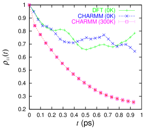
Figure 2: Time evolution of the excited density matrix for NMA-D in vacuum (DFT and CHARMM) at 0K, and for NMA-D in heavy water (CHARMM) at 300K. The level of DFT is B3LYP/6-31+G(d).

Table 2: The most dominant VER pathways for the amide I mode of NMA-D in heavy water. $\Delta\omega$ is defined by $|\omega_{S}-\omega_{\alpha}-\omega_{\beta}|$.

Mode combination ($\alpha,\beta$)	frequency (cm-1)	Contribution to $s(t)$	$\Delta\omega$ (cm-1)
1143 + 1143	778.6 + 778.6	0.04	125.7
1147 + 1134	1085.3 + 570.0	0.04	27.6
1147 + 1135	1085.3 + 570.9	0.01	26.6
1147 + 1136	1085.3 + 578.8	0.02	18.8
1147 + 1137	1085.3 + 581.3	0.03	16.2
1147 + 1140	1085.3 + 612.1	0.46	14.5
1148 + 1132	1127.8 + 558.5	0.01	3.4
1148 + 1134	1127.8 + 570.0	0.11	14.9
1148 + 1135	1127.8 + 570.9	0.03	15.9

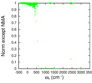
Figure 3: Norm of the eigenvectors (normal modes) with the exception of the contribution from NMA-D, which is defined by $\sum_{i\in{\rm Water}}(x_{i}^{2}+y_{i}^{2}+z_{i}^{2})$, where $i$ comes from water degrees of freedom alone.

Table 3: The most localized modes around the CO bond in NMA-D. The norm is defined by $\sum_{i\in{\rm CObond}}(x_{i}^{2}+y_{i}^{2}+z_{i}^{2})$. The 1345th mode is the amide I mode.

Mode index $\alpha$	frequency (cm-1)	Contribution to norm
1134	570.0	0.14
1140	612.1	0.26
1142	771.2	0.35
1143	778.6	0.41
1146	1013.6	0.13
1147	1085.3	0.26
1148	1127.8	0.17
1340	1452.1	0.36
1345	1689.6	0.92

Table 4: The most dominant VER pathways for NMA-D in vacuum with the ab initio potential (B3LYP/6-31+G(d)).

Mode combination ($\alpha,\beta$)	frequency (cm-1)	Contribution to $s(t)$	$\Delta\omega$ (cm-1)
9 + 9	868.7 + 868.7	0.13	2.7
13 + 8	1144.5+ 620.0	0.02	29.8

Table 5: The most dominant VER pathways for NMA-D in vacuum with the CHARMM force field.

Mode combination ($\alpha,\beta$)	frequency (cm-1)	Contribution to $s(t)$	$\Delta\omega$ (cm-1)
8 + 8	741.9 +741.9	0.02	194.1
14 + 6	1088.5+536.3	0.08	53.1
14 + 8	1088.5+741.9	0.02	152.5
15 + 7	1123.5+575.9	0.08	21.6

III.4 Dephasing properties of NMA-D

We now consider the dephasing properties of the amide I mode. The off-diagonal density matrix is written as

$$\rho_{10}(t)=\frac{1}{2}e^{-i\tilde{\omega}_{S}t}[1-r^{(2)}_{FF}(t)-r^{(2)}_{GG}(t)-r^{(2)}_{FG}(t)]\simeq\frac{1}{2}e^{-i\tilde{\omega}_{S}t-r^{(2)}_{FF}(t)-r^{(2)}_{GG}(t)-r^{(2)}_{FG}(t)}$$ (47)

and we analyze each contribution to the density matrix seperately.

In Fig. 4, we show the result with $R_{c}=10$ Å  and $\omega_{c}=10$ cm^-1. We can see that the following relation holds

$${\rm Re}\{r^{(2)}_{FF}(t)\}\simeq s(t)/2\simeq t/(2T_{1}).$$ (48)

If we further assume that ${\rm Re}\{r^{(2)}_{GG}(t)\}\simeq t/T_{2}^{*}$ and ${\rm Re}\{r^{(2)}_{FG}(t)\}\simeq 0$, we have

$$\frac{1}{T_{2}}=\frac{1}{2T_{1}}+\frac{1}{T_{2}^{*}}.$$ (49)

This is a standard expression connecting $T_{1}$ and $T_{2}$ Mchale , and holds under the Markov approximation. We can see that ${\rm Re}\{r^{(2)}_{FG}(t)\}\simeq 0$ holds, but it is difficult to judge whether ${\rm Re}\{r^{(2)}_{GG}(t)\}\simeq t/T_{2}^{*}$ holds or not.

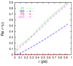
Figure 4: Dephasing properties of the amide I mode of NMA-D in heavy water.

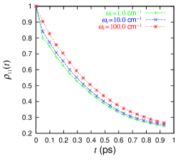
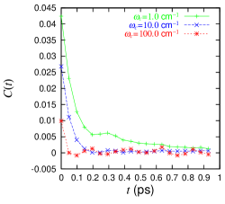
Figure 5: Left: VER (left) and frequency auto correlation calculations (right) at 300K with different cut-off frequencies $\omega_{c}$.

There are more serious problems: as mentioned by Mikami and Okazaki MO04 , the diagonal terms contribute most for dephasing, i.e., the second term in Eq. (37) is a dominant contribution for dephasing. Furthermore, the coefficients are dominant factors, so this means that the low frequency (and thus delocalized) modes contribute most. In this paper, we have employed two cut-off parameters: $R_{c}$ and $\omega_{c}$. If $R_{c}$ is large enough, it is fine, but the choice of $\omega_{c}$ can be arbitrary. Figure 5 shows the dependence of the results on $\omega_{c}$. The VER results do not depend on the choice of $\omega_{c}$ because there is a resonant condition which should be met, but the dephasing results do. We need to be cautious in the interpretation of our results for dephasing. One way to get rid of this problem is to go back to the original expression Eq. (34) using the force and force-constant autocorrelation functions $\langle\delta{\cal F}(t)\delta{\cal F}(0)\rangle$ and $\langle\delta{\cal G}(t)\delta{\cal G}(0)\rangle$. Here $r^{(2)}_{GG}(t)$ is calculated as time integral of these correlation functions, which can be calculated using classical mechanics. This is in the same spirit as the quantum correction factor method SP01 , which is an approximation to quantum effects. In this case, we only need to consider the zero frequency component, so the classical mechanics should work well and quantum effects should be less important.

III.5 Discussions

We found that there are several resonant modes in NMA-D, which form the main VER pathways within the molecule. Gerber and coworkers reported that the amide I mode in NMA is very weakly coupled to other modes GCG02 . We expect that this discrepancy results from (a) the use of only pair interactions between normal modes to reduce the computational cost, (b) the level of the ab initio method: they used MP2/DZP whereas we used B3LYP/6-31+G(d), and (c) the criterion of the mode-mode coupling: their criterion is not directly related to VER.

It is important and interesting to clarify the nature of VER in the amide I mode in more detail. Note the importance of the system anharmonicity. The effect of the system anharmonicity defined in Eq. (59) is very weak for the CHARMM case: $\varepsilon=10^{-5}$, but it is not for the ab initio case: $\varepsilon=10^{-2}$. According to Eq. (62), this anharmonicity shifts the system frequency by 0.6%, which amounts to 10 cm^-1. The resonant condition changes compared to the case without anharmonicity. Of course, dephasing is also affected by this amount of anharmonicity. To address these issues, we must develop QM/MM type methods, which will be described elsewhere. Another interesting system to investigate anharmonicity is a highly excited bond such as the highly excited CO bond in myoglobin VFVAMJ04 .

It is important to assess our strategy: our perturbative expansion and cut-off strategy are approximate. It would be profitable and interesting to compare this strategy with others, including the time-dependent vibrational self-consistent field methods JG99 ; FYZSH , the semiclassical method Geva , and the path integral method Krilov . The application of our strategy to protein systems, including cytochrome c, will be described elsewhere Matt .

IV Summary

In this paper, we have derived formulas for VER and dephasing for an anharmonic (cubic) oscillator coupled to a harmonic bath through 3rd and 4th order coupling elements. We employed time-dependent perturbation theory and did not take the infinite time limit as is done in the derivation of the Maradudin-Fein formula. Hence our formulas do not assume the Markov properties of the system, and can describe short time behavior that can be important for VER and dephasing properties of localized modes in peptides or proteins. Our final results are the VER formula [Eq. (26)] and dephasing formula [Eq. (31) with Eqs. (36)-(38)]. As a test case, we have studied the amide I mode of $N$-methylacetamide in heavy water. We found that the VER time is 0.5 ps at 300K, which is in good accord with the experimental value, and clarified that the VER mechanism is mainly localized around the peptide bond in NMA-D; VER is dominated by IVR within the molecule. We also investigated the dephasing properties of the amide I mode, and met with some problems. We proposed a new method to overcome these problems using classical correlation function calculations.

Appendix A System parameters for a cubic oscillator

We assume that the system-bath interaction can be Taylor expanded using the bath coordinate $q_{\alpha}$, and that the fluctuating force and the fluctuating force constant can be expressed as

$$\delta{\cal F} = \sum_{\alpha,\beta}C_{S\alpha\beta}(q_{\alpha}q_{\beta}-\langle q_{\alpha}q_{\beta}\rangle),$$ (50)

$$\delta{\cal G} = \sum_{\alpha,\beta}C_{SS\alpha\beta}(q_{\alpha}q_{\beta}-\langle q_{\alpha}q_{\beta}\rangle)+\sum_{\alpha}C_{SS\alpha}q_{\alpha}.$$ (51)

In real molecular systems such as peptides or proteins, the coefficients in ${\cal V}$ and the anharmonicity parameter in ${\cal H}_{f}$ are calculated as

$$C_{S\alpha\beta} = -\frac{1}{2}\frac{\partial^{3}V}{\partial q_{S}\partial q_{\alpha}\partial q_{\beta}},$$ (52)

$$C_{SS\alpha} = \frac{1}{2}\frac{\partial^{3}V}{\partial q_{S}^{2}\partial q_{\alpha}},$$ (53)

$$C_{SS\alpha\beta} = \frac{1}{4}\frac{\partial^{4}V}{\partial q_{S}^{2}\partial q_{\alpha}\partial q_{\beta}},$$ (54)

$$f = \frac{\partial^{3}V}{\partial q_{S}^{3}}$$ (55)

where $V$ represents a potential function for the system considered. This potential function can be an empirical force field (CHARMM, Amber) or an ab initio potential calculated by any level of theory.

Assuming that the cubic anhamonicity $f$ in the system is small, we use the time-independent perturbation theory to calculate the eigen energies and vectors. We quote from J.J. Sakurai JJ :

$$E_{n} = E^{(0)}_{n}+V_{nn}+\sum_{k\neq n}\frac{|V_{nk}|^{2}}{E^{(0)}_{n}-E^{(0)}_{k}},$$ (56)

$$|n\rangle = |n^{(0)}\rangle+\sum_{k\neq n}|k^{(0)}\rangle\frac{V_{kn}}{E^{(0)}_{n}-E^{(0)}_{k}}$$ (57)

$$+\left(\sum_{k\neq n}\sum_{l\neq n}|k^{(0)}\rangle\frac{V_{kl}V_{ln}}{(E^{(0)}_{n}-E^{(0)}_{k})(E^{(0)}_{n}-E^{(0)}_{l})}-\sum_{k\neq n}|k^{(0)}\rangle\frac{V_{nn}V_{kn}}{(E^{(0)}_{n}-E^{(0)}_{k})^{2}}\right)$$

where $E^{(0)}_{n}=\hbar\bar{\omega}_{S}(n+1/2)$, $|k^{(0)}\rangle$ is the $k$-th eigenfunction of the harmonic oscillator, and

$$V_{kn} = \frac{f}{6}\langle k^{(0)}|\bar{q}_{S}^{3}|n^{(0)}\rangle$$ (58)

$$= \hbar\bar{\omega}_{S}\varepsilon\left[\sqrt{n(n-1)(n-2)}\delta_{k,n-3}+3n\sqrt{n}\delta_{k,n-1}\right.$$

$$\left.+3(n+1)\sqrt{n+1}\delta_{k,n+1}+\sqrt{(n+1)(n+2)(n+3)}\delta_{k,n+3}\right]$$

where

$$\varepsilon=\frac{1}{\hbar\bar{\omega}_{S}}\frac{f}{6}\left(\frac{\hbar}{2\bar{\omega}_{S}}\right)^{3/2}$$ (59)

is a dimensionless paramater representing the strength of the anharmonicity of the system. Note that $V_{kn}$ becomes nonzero only when $|k-n|=1$ or $|k-n|=3$.

We explicitly have

$$E_{0} = \frac{\hbar\bar{\omega}_{S}}{2}-\frac{|V_{01}|^{2}}{\hbar\bar{\omega}_{S}}-\frac{|V_{03}|^{2}}{3\hbar\bar{\omega}_{S}}=\frac{\hbar\bar{\omega}_{S}}{2}(1-22\varepsilon^{2}),$$ (60)

$$E_{1} = \frac{3\hbar\bar{\omega}_{S}}{2}+\frac{|V_{10}|^{2}}{\hbar\bar{\omega}_{S}}-\frac{|V_{12}|^{2}}{\hbar\bar{\omega}_{S}}-\frac{|V_{14}|^{2}}{3\hbar\bar{\omega}_{S}}=\frac{\hbar\bar{\omega}_{S}}{2}(3-142\varepsilon^{2}).$$ (61)

The anharmonicity-corrected frequency is

$$\tilde{\omega}_{S}=\frac{E_{1}-E_{0}}{\hbar}=\bar{\omega}_{S}(1-60\varepsilon^{2}).$$ (62)

Next we calculate the matrix elements for ${q}_{S}$ and ${q}_{S}^{2}$. We write the eigenfunctions:

$$|0\rangle = |0^{(0)}\rangle+\sum_{k=1,3}|k^{(0)}\rangle\frac{V_{k0}}{E^{(0)}_{0}-E^{(0)}_{k}}+\sum_{k,l\in S_{0}}|k^{(0)}\rangle\frac{V_{kl}V_{l0}}{(E^{(0)}_{0}-E^{(0)}_{k})(E^{(0)}_{0}-E^{(0)}_{l})},$$ (63)

$$|1\rangle = |1^{(0)}\rangle+\sum_{k=0,2,4}|k^{(0)}\rangle\frac{V_{k1}}{E^{(0)}_{1}-E^{(0)}_{k}}+\sum_{k,l\in S_{1}}|k^{(0)}\rangle\frac{V_{kl}V_{l1}}{(E^{(0)}_{1}-E^{(0)}_{k})(E^{(0)}_{1}-E^{(0)}_{l})}$$ (64)

where $S_{0}$ represents $(l=1,k=2)$ or $(l=1,k=4)$ or $(l=3,k=2)$ or $(l=3,k=4)$ or $(l=3,k=6)$, and $S_{1}$ does $(l=0,k=3)$ or $(l=2,k=3)$ or $(l=2,k=5)$ or $(l=4,k=3)$ or $(l=4,k=5)$, or $(l=4,k=7)$. Note that these eigenvectors are not normalized, so we need to renormalize them before or after calculations.

After some lengthy but straighforward calculations, we have

$$(q_{S})_{10} = \langle 1|\bar{q}_{S}+b|0\rangle=(q_{S})_{01}=a(1+22\varepsilon^{2}),$$ (65)

$$(q_{S})_{00} = \langle 0|\bar{q}_{S}+b|0\rangle=b-6a\varepsilon,$$ (66)

$$(q_{S})_{11} = \langle 1|\bar{q}_{S}+b|1\rangle=b-18a\varepsilon,$$ (67)

$$(q^{2}_{S})_{10} = \langle 1|(\bar{q}_{S}+b)^{2}|0\rangle=(q^{2}_{S})_{01}=2ab-20a^{2}\varepsilon+44ab\varepsilon^{2},$$ (68)

$$(q^{2}_{S})_{00} = \langle 0|(\bar{q}_{S}+b)^{2}|0\rangle=a^{2}+b^{2}-12ab\varepsilon+88a^{2}\varepsilon^{2},$$ (69)

$$(q^{2}_{S})_{11} = \langle 1|(\bar{q}_{S}+b)^{2}|1\rangle=3a^{2}+b^{2}-36ab\varepsilon+568a^{2}\varepsilon^{2}$$ (70)

where

$$a=\sqrt{\frac{\hbar}{2\bar{\omega}_{S}}}$$ (71)

is the fundamental length charactering the system oscillator.

Appendix B The coefficients used in the formulas

Using the expression derived previously for the force-force correlation function FBS05a , the coefficients in our VER and dephasing formulas are expressed as

$$\mathbf{C}^{\alpha\beta} = \left(\begin{array}[]{cc}C^{\alpha\beta}_{--}&C^{\alpha\beta}_{+-}\\ C^{\alpha\beta}_{+-}&C^{\alpha\beta}_{++}\\ \end{array}\right)=\left\{(q_{S})_{10}C_{S\alpha\beta}-(q^{2}_{S})_{10}C_{SS\alpha\beta}\right\}^{2}\mathbf{S}^{\alpha\beta},$$ (74)

$$\mathbf{D}^{R\alpha\beta} = \left(\begin{array}[]{cc}D^{R\alpha\beta}_{--}&D^{R\alpha\beta}_{+-}\\ D^{R\alpha\beta}_{+-}&D^{R\alpha\beta}_{++}\\ \end{array}\right)$$ (77)

$$= \left\{[(q_{S})_{11}-(q_{S})_{00}]C_{S\alpha\beta}-[(q^{2}_{S})_{11}-(q^{2}_{S})_{00}]C_{SS\alpha\beta}\right\}^{2}\mathbf{S}^{\alpha\beta},$$ (78)

$$\mathbf{D}^{I\alpha\beta} = \left(\begin{array}[]{cc}D^{I\alpha\beta}_{--}&D^{I\alpha\beta}_{+-}\\ D^{I\alpha\beta}_{+-}&D^{I\alpha\beta}_{++}\\ \end{array}\right)$$ (82)

$$= \left\{[(q_{S})_{11}-(q_{S})_{00}]C_{S\alpha\beta}-[(q^{2}_{S})_{11}-(q^{2}_{S})_{00}]C_{SS\alpha\beta}\right\}$$

$$\times\left\{[(q_{S})_{11}+(q_{S})_{00}]C_{S\alpha\beta}-[(q^{2}_{S})_{11}+(q^{2}_{S})_{00}]C_{SS\alpha\beta}\right\}\mathbf{S}^{\alpha\beta},$$

$$\mathbf{E}^{\alpha\beta} = \left(\begin{array}[]{cc}E^{\alpha\beta}_{--}&E^{\alpha\beta}_{+-}\\ E^{\alpha\beta}_{+-}&E^{\alpha\beta}_{++}\\ \end{array}\right)$$ (86)

$$= \left\{[(q_{S})_{11}-(q_{S})_{00}]C_{S\alpha\beta}-[(q^{2}_{S})_{11}-(q^{2}_{S})_{00}]C_{SS\alpha\beta}\right\}$$

$$\times\left\{(q_{S})_{10}C_{S\alpha\beta}-(q^{2}_{S})_{10}C_{SS\alpha\beta}\right\}\mathbf{S}^{\alpha\beta},$$

$$\mathbf{S}^{\alpha\beta} = \frac{\hbar^{2}}{2\omega_{\alpha}\omega_{\beta}}\left(\begin{array}[]{cc}(1+n_{\alpha})(1+n_{\beta})&2(1+n_{\alpha})n_{\beta}\\ 2(1+n_{\alpha})n_{\beta}&n_{\alpha}n_{\beta}\\ \end{array}\right),$$ (89)

$$\mathbf{C}^{\alpha} = \left(\begin{array}[]{c}C^{\alpha}_{-}\\ C^{\alpha}_{+}\\ \end{array}\right)=(q_{S}^{2})_{10}^{2}C_{SS\alpha}^{2}\mathbf{R}^{\alpha},$$ (92)

$$\mathbf{D}^{R\alpha} = \left(\begin{array}[]{c}D^{R\alpha}_{-}\\ D^{R\alpha}_{+}\\ \end{array}\right)=[(q_{S}^{2})_{11}-(q_{S}^{2})_{00}]^{2}C_{SS\alpha}^{2}\mathbf{R}^{\alpha},$$ (95)

$$\mathbf{D}^{I\alpha} = \left(\begin{array}[]{c}D^{I\alpha}_{-}\\ D^{I\alpha}_{+}\\ \end{array}\right)=[(q_{S}^{2})_{11}-(q_{S}^{2})_{00}][(q_{S}^{2})_{11}+(q_{S}^{2})_{00}]C_{SS\alpha}^{2}\mathbf{R}^{\alpha},$$ (98)

$$\mathbf{E}^{\alpha} = \left(\begin{array}[]{c}E^{\alpha}_{-}\\ E^{\alpha}_{+}\\ \end{array}\right)=[(q_{S}^{2})_{11}-(q_{S}^{2})_{00}](q_{S}^{2})_{10}C_{SS\alpha}^{2}\mathbf{R}^{\alpha},$$ (101)

$$\mathbf{R}^{\alpha} = \frac{\hbar}{2\omega_{\alpha}}\left(\begin{array}[]{c}1+n_{\alpha}\\ n_{\alpha}\\ \end{array}\right)$$ (104)

where $n_{\alpha}=1/(e^{\beta\hbar\omega_{\alpha}}-1)$ is the thermal phonon number.

To calculate $\bar{\omega}_{S}$ and $b$ in Eqs. (6) and (7), we use the following

$$\langle{\cal F}(t)\rangle = \langle{\cal F}(0)\rangle=\frac{\hbar}{2}\sum_{\alpha}\frac{C_{S\alpha\alpha}}{\omega_{\alpha}}(1+2n_{\alpha}),$$ (105)

$$\langle{\cal G}(t)\rangle = \langle{\cal G}(0)\rangle=\frac{\hbar}{2}\sum_{\alpha}\frac{C_{SS\alpha\alpha}}{\omega_{\alpha}}(1+2n_{\alpha}).$$ (106)

References

- (1) See, e.g., H. Fujisaki and J.E. Straub, Proc. Natl. Acad. Sci. USA 102, 6726 (2005) and references therein; e-print q-bio.BM/0412048.
- (2) D.W. Oxtoby, Adv. Chem. Phys. 40, 1 (1979); ibid. 47, 487 (1981).
- (3) R. Rey, K.B. Moller, and J.T. Hynes, Chem. Rev. 104, 1915 (2004); K.B. Moller, R. Rey, and J.T. Hynes, J. Phys. Chem. A 108, 1275 (2004).
- (4) C.P. Lawrence and J.L. Skinner, J. Chem. Phys. 117, 5827 (2002); ibid. 117, 8847 (2002); ibid. 118, 264 (2003); A. Piryatinski, C.P. Lawrence, and J.L. Skinner, ibid. 118, 9664 (2003); ibid. 118, 9672 (2003); C.P. Lawrence and J.L. Skinner, ibid. 119, 1623 (2003); ibid. 119, 3840 (2003).
- (5) D.E. Sagnella and J.E. Straub, Biophys. J. 77, 70 (1999); L. Bu and J.E. Straub, ibid. 85, 1429 (2003).
- (6) D.M. Leitner, Adv. Chem. Phys. 130B, 205 (2005).
- (7) H. Fujisaki, L. Bu, and J.E. Straub, Adv. Chem. Phys. 130B, 179 (2005); e-print q-bio.BM/0403019.
- (8) H. Fujisaki, L. Bu, and J.E. Straub, in Normal Mode Analysis: Theory and Applications to Biological and Chemical Systems, edited by Q. Cui and I. Bahar (2005); e-print q-bio.BM/0408023.
- (9) D.M. Leitner, Chem. Phys. Lett. 359, 434 (2002).
- (10) T. Mikami and S. Okazaki, J. Chem. Phys. 121, 10052 (2004).
- (11) U. Weiss, Quantum Dissipative Systems, 2nd Ed. World Scientific Publishing, Singapore (1999).
- (12) R. Xu, Y.J. Yan, and O. Kühn, Europhys. J. D 19, 293 (2002).
- (13) C. Ventalon, J.M. Fraser, M.H. Vos, A. Alexandrou, J.L. Martin, and M. Joffre, Proc. Natl. Acad. Sci. USA 101, 13216 (2004); O. Kühn, Chem. Phys. Lett. 402, 48 (2005).
- (14) H. Fujisaki, T. Miyadera, and A. Tanaka, Phys. Rev. E. 67, 066201 (2003).
- (15) S.K. Gregurick, G.M. Chaban, and R.B. Gerber, J. Phys. Chem. A 106, 8696 (2002).
- (16) P.H. Nguyen and G. Stock, J. Chem. Phys. 119, 11350 (2003).
- (17) J.R. Schmidt, S.A. Corcelli, and J.L. Skinner, J. Chem. Phys. 121, 8887 (2004).
- (18) M.T. Zanni, M.C. Asplund, and R.M. Hochstrasser, J. Chem. Phys. 114, 4579 (2001).
- (19) S. Woutersen, R. Pfister, P. Hamm, Y. Mu, D.S. Kosov, and G. Stock, J. Chem. Phys. 117, 6833 (2002).
- (20) B.R. Brooks, R.E. Bruccoleri, B.D. Olafson, D.J. States, S. Swaminathan, and M. Karplus, J. Comp. Chem. 4, 187 (1983); A.D. MacKerell, Jr., B. Brooks, C.L. Brooks III, L. Nilsson, B. Roux, Y. Won, and M. Karplus, in The Encyclopedia of Computational Chemistry, 1, 271, edited by P.v.R. Schleyer et al., John Wiley & Sons: Chichester (1998).
- (21) M. Cho, G.R. Fleming, S. Saito, I. Ohmine, and R.M. Stratt, J. Chem. Phys. 100, 6672 (1994); T. Keyes, J. Phys. Chem. A 101, 2921 (1997).
- (22) H.-P. Breuer and F. Petruccione, The Theory of Open Quantum Systems, Oxford University Press, New York (2002); in Quantum computing and quantum bits in mesoscopic systems, edited by A. Leggett, B. Ruggiero and P. Silvestrini, 263-271, Kluwer Academic/Plenum Publishers, New York (2004).
- (23) F. Intravaia, S. Maniscalco, and A. Messina, Eur. Phys. J. B 32, 97 (2003).
- (24) K. Yagi, K. Hirao, T. Taketsugu, M.W. Schmidt, and M.S. Gordon, J. Chem. Phys. 121, 1383 (2004).
- (25) H. Guo and M. Karplus, J. Phys. Chem. 96, 7273 (1992).
- (26) K. Moritsugu, O. Miyashita, and A. Kidera, Phys. Rev. Lett. 85, 3970 (2000).
- (27) P. Mukherjee, A.T. Krummel, E.C. Fulmer, I. Kass, I.T. Arkin, and M.T. Zanni, J. Chem. Phys. 120, 10215 (2004).
- (28) A. Xie, L. van der Meer, W. Hoff, and R.H. Austin, Phys. Rev. Lett. 84, 5435 (2000).
- (29) J.L. McHale, Molecular Spectroscopy, Prentice-Hall, Inc. (1999).
- (30) J.L. Skinner and K. Park, J. Phys. Chem. B 105, 6716 (2001).
- (31) P. Jungwirth and R.B. Gerber, Chem. Rev. 99, 1583 (1999); C. Iung, F. Gatti, H.-D. Meyer, J. Chem. Phys. 120, 6992 (2004); F. Gatti and H-D. Meyer, Chem. Phys. 304, 3 (2004).
- (32) H. Fujisaki, K. Yagi, Y. Zhang, J.E. Straub, and K. Hirao, unpublished.
- (33) Q. Shi and E. Geva, J. Phys. Chem. A 107, 9059 (2003); ibid. 107, 9070 (2003); J. Chem. Phys. 119, 9030 (2003).
- (34) G. Krilov, E. Sim, and B.J. Berne, Chem. Phys. 268, 21 (2001); E. Rabani, D.R. Reichman, G. Krilov, and B.J. Berne, Proc. Natl. Acad. Sci. USA 99, 1129 (2002).
- (35) M. Cremeens, H. Fujisaki, Y. Zhang, J. Zimmermann, L.B. Sagle, S. Matsuda, P.E. Dawson, J.E. Straub, and F.E. Romesberg, unpublished.
- (36) J.J. Sakurai, Modern Quantum Mechanics, Benjamin/Cummings, 2nd edition (1994).