Quantum mechanical calculation of the effects of stiff and rigid constraints in the conformational equilibrium of the Alanine dipeptide

Abstract

If constraints are imposed on a macromolecule, two inequivalent classical models may be used: the stiff and the rigid one. This work studies the effects of such constraints on the Conformational Equilibrium Distribution (CED) of the model dipeptide HCO-L-Ala-NH₂ without any simplifying assumption. We use ab initio Quantum Mechanics calculations including electron correlation at the MP2 level to describe the system, and we measure the conformational dependence of all the correcting terms to the naive CED based in the Potential Energy Surface (PES) that appear when the constraints are considered. These terms are related to mass-metric tensors determinants and also occur in the Fixman’s compensating potential. We show that some of the corrections are non-negligible if one is interested in the whole Ramachandran space. On the other hand, if only the energetically lower region, containing the principal secondary structure elements, is assumed to be relevant, then, all correcting terms may be neglected up to peptides of considerable length. This is the first time, as far as we know, that the analysis of the conformational dependence of these correcting terms is performed in a relevant biomolecule with a realistic potential energy function.
PACS: 87.14.Ee, 87.15.-v, 87.15.Aa, 87.15.Cc, 89.75.-k

1 Introduction

In computer simulations of large complex systems, such as macromolecules and, specially, proteins [1, 2, 3, 4, 5, 6], one of the main bottlenecks to design efficient algorithms is the necessity to sample an astronomically large conformational space [3, 7]. In addition, being the typical timescales of the different movements in a wide range, demandingly small timesteps must be used in Molecular Dynamics simulations in order to properly account for the fastest modes, which lie in the femtosecond range. However, most of the biological interesting behaviour (allosteric transitions, protein folding, enzymatic catalysis) is related to the slowest conformational changes, which occur in the timescale of milliseconds or even seconds [8, 9, 10, 4, 11]. Fortunately, the fastest modes are also the most energetic ones and are rarely activated at room temperature. Therefore, in order to alleviate the computational problems and also simplify the images used to think about these elusive systems, one may naturally consider the reduction of the number of degrees of freedom describing macromolecules via the imposition of constraints [12].

How to study the conformational equilibrium of these constrained systems has been an object of much debate [13, 14, 15, 16, 17]. Two different classical models exist in the literature which are conceptually [18, 19, 13, 14, 15, 16] and practically [20, 21, 6, 13, 22, 23, 24] inequivalent. In the classical rigid model, the constraints are assumed to be exact and all the velocities that are orthogonal to the hypersurface defined by them vanish. In the classical stiff model, on the other hand, the constraints are assumed to be approximate and they are implemented by a steep potential that drives the system to the constrained hypersurface. In this case, the orthogonal velocities are activated and may act as “heat containers”.

In this work, we do not address the question of which model is a better approximation of physical reality. Although, in the literature, it is commonly assumed (often implicitly) that the classical stiff model should be taken as a reference [20, 9, 19, 26, 6, 22, 16], we believe that this opinion is much influenced by the use of popular classical force fields [27, 28, 6, 29, 30, 31, 32, 33, 34, 35, 36, 37] (which are stiff by construction) and by the goal of reproducing their results at a lower computational cost, i.e., using rigid Molecular Dynamics simulations [38, 8, 9, 25, 19, 39, 4, 5, 40, 21, 41, 26, 22, 23, 14, 42]. In our opinion, the question whether the rigid or the stiff model should be used to approximate the real quantum mechanical statistics of an arbitrary organic molecule has not been satisfactorily answered yet. For discussions about the topic, see references [18, 43, 44, 45, 13, 14, 15, 17]. In this work, we adopt the cautious position that any of the two models may be useful in certain cases or for certain purposes and we study them both on equal footing. Our concern is, then, to study the effects that either way of imposing constraints causes in the conformational equilibrium of macromolecules.

In the Born-Oppenheimer approximation [46] customarily used in Quantum Mechanics and in the majority of the classical force fields, the relevant degrees of freedom are the Euclidean (also called Cartesian by some authors) $3n$ coordinates of the $n$ nuclei. However, it is frequent to define a different set of coordinates in which the overall translation and rotation of the system are distinguished and the remaining $3n-6$ degrees of freedom are chosen (according to different prescriptions as internal coordinates, which are simple geometrical parameters (typically consisting of bond lengths, bond angles and dihedral angles) that describe the internal structure of the system [47].

In macromolecules, the natural constraints are those derived from the relative rigidity of the internal covalent structure of groups of atoms that share a common center (and also from the rigidity of rotation around double or triple bonds) compared to the energetically “cheaper” rotation around single bonds. In internal coordinates, these chemical constraints may be directly implemented by asking that some conveniently selected hard coordinates (normally, bond lengths, bond angles and some dihedrals) have constant values or values that depend on the remaining soft coordinates (see ref. [15] for a definition). In Euclidean coordinates, on the other hand, the expression of the constraints is more cumbersome and complicated procedures [25, 48, 40, 26, 49, 50] must be used at each timestep to implement them in Molecular Dynamics simulations. This is why, in the classical stiff model, as well as in the rigid one, it is common to use internal coordinates and they are also the choice throughout this work.

In the equilibrium Statistical Mechanics of both the stiff and rigid models, the marginal probability density in the coordinate part of the phase space in these internal coordinates is not proportional to the naive $\exp[-\beta V_{\Sigma}(q^{i})]$, where $V_{\Sigma}(q^{i})$ denotes the potential energy on the constrained hypersurface. Instead, some correcting terms that come from different sources must be added to the potential energy $V_{\Sigma}(q^{i})$ [18, 51, 19, 39, 52, 13, 15]. These terms involve determinants of mass-metric tensors and also of the Hessian matrix of the constraining part of the potential (see sec. 2). If Monte Carlo simulations in the coordinate space are to be performed [53, 54, 5, 55, 56, 57] and the probability densities that correspond to any of these two models sampled, the corrections should be included or, otherwise, showed to be negligible.

Additionally, the three different correcting terms are involved in the definition of the so-called Fixman’s compensating potential [16], which is frequently used to reproduce the stiff equilibrium distribution using rigid Molecular Dynamics simulations [51, 38, 9, 19, 39, 21, 22, 23, 14, 42].

Customarily in the literature, some of these corrections to the potential energy are assumed to be independent of the conformation and thus dropped from the basic expressions. Also, subtly entangled to the assumptions underlying many classical results, a second type of approximation is made that consists of assuming that the equilibrium values of the hard coordinates do not depend on the soft coordinates.

In this work, we measure the conformational dependence of all correcting terms and of the Fixman’s compensating potential in the model dipeptide HCO-L-Ala-NH₂ without any simplifying assumption. The potential energy function is considered to be the effective Born-Oppenheimer potential for the nuclei derived from ab initio quantum mechanical calculations including electron correlation at the MP2 level. We also repeat the calculations, with the same basis set (6-31++G(d,p)) and at the Hartree-Fock level of the theory in order to investigate if this less demanding method without electron correlation may be used in further studies. It is the first time, as far as we are aware, that this type of study is performed in a relevant biomolecule with a realistic potential energy function.

In sec. 2, we introduce the notation to be used and derive the Statistical Mechanics formulae of the rigid and stiff models in the general case. In sec. 3, we describe the computational methods used and we summarize the factorization of the external coordinates presented in ref. [58]. Sec. 4 is devoted to the presentation and discussion of the assessment of the approximation that consists of neglecting the different corrections to the potential energy in the model dipeptide HCO-L-Ala-NH₂, without any simplifying assumption, which is the central aim of this work. The conclusions are summarized in sec. 5. Finally, in the appendix, we discuss the use of the different approximations in the literature and we give a precise definition of exactly and approximately separable hard and soft coordinates which will shed some light on the relation between the different types of simplifications aforementioned.

2 Theory

First of all, it is convenient to introduce certain notational conventions that will be used extensively in the rest of the work:

• The system under scrutiny will be a set of $n$ mass points termed atoms. The Euclidean coordinates of the atom $\alpha$ in a set of axes fixed in space are denoted by $\vec{x}_{\alpha}$. The subscript $\alpha$ runs from 1 to $n$.

• The curvilinear coordinates suitable to describe the system will be denoted by $q^{\mu},\ \mu=1,\ldots,3n$ and the set of Euclidean coordinates by $x^{\mu}$ when no explicit reference to the atoms index needs to be made. We shall often use $N:=3n$ for the total number of degrees of freedom.

• The coordinates $q^{\mu}$ are split into $(q^{A},q^{a}),\ a=7,\dots,N$. The first six are termed external coordinates and are denoted by $q^{A}$. They describe the overall position and orientation of the system with respect to a frame fixed in space (see ref. 58 for further details). The coordinates $q^{a}$ are said internal coordinates and determine the positions of the atoms in the frame fixed in the system. They parameterize what we shall call the internal subspace or conformational space, denoted by $\mathcal{I}$ and the coordinates $q^{A}$ parameterize the external subspace, denoted by $\mathcal{E}$.

• The general set-up of the problem may be described as follows: Instead of us being interested on the conformational equilibrium of the system in the external subspace $\mathcal{E}$ plus the whole internal subspace $\mathcal{I}$ (i.e., the whole space, denoted by $\mathcal{E}\times\mathcal{I}$), we wish to find the probability density on a hypersurface $\Sigma\subset\mathcal{I}$ of dimension $M$ (plus the external subspace $\mathcal{E}$), i.e., on $\mathcal{E}\times\Sigma$.

• In typical internal coordinates $q^{a}$, normally consisting of bond lengths, bond angles and dihedral angles (see ref. 59 and references therein), the hypersurface $\Sigma$ is described via $L:=N-M-6$ constraints:

  $$q^{I}=f^{I}(q^{i})\qquad I=M+7,\ldots,N\ ,$$ (2.1)

  where the $q^{a}$ are split into $q^{a}\equiv(q^{i},q^{I})$, and the $q^{i}$, $i=7,\ldots,M+6$, which parameterize $\Sigma$, are called internal soft coordinates, whereas the $q^{I}$ are termed hard coordinates. The external coordinates $q^{A}$, together with the $q^{i}$, form the whole set of soft coordinates, denoted by $q^{u}\equiv(q^{A},q^{i})$, $u=1,\ldots,M+6$.

In table 1, a summary of the indices used is given.

Indices	Range	Number	Description
$\alpha,\beta,\gamma,\ldots$	$1,\ldots,n$	$n$	Atoms
$\mu,\nu,\rho,\ldots$	$1,\ldots,N$	$N=3n$	All coordinates
$A,B,C,\ldots$	$1,\ldots,6$	6	External coordinates
$a,b,c,\ldots$	$7,\ldots,N$	$N-6$	Internal coordinates
$i,j,k,\ldots$	$7,\ldots,M+6$	$M$	Soft internal coordinates
$I,J,K,\ldots$	$M+7,\ldots,N$	$L=N-M-6$	Hard internal coordinates
$u,v,w,\ldots$	$1,\ldots,M+6$	$M+6$	All soft coordinates

Table 1: Definition of the indices used.

2.1 Classical stiff model

In the classical stiff model, the constraints in eq. 2.1 are implemented by imposing an strong energy penalization when the internal conformation of the system, described by $q^{a}$, departs from the constrained hypersurface $\Sigma$. To ensure this, we must have that the potential energy function in $\mathcal{I}$ satisfies certain conditions. First, we write the potential $V(q^{a})$ as follows:

$$V(q^{i},q^{I})=\underbrace{V\big{(}q^{i},f^{I}(q^{i})\big{)}}_{\displaystyle V_{\Sigma}(q^{i})}+\underbrace{\Big{[}V(q^{i},q^{I})-V\big{(}q^{i},f^{I}(q^{i})\big{)}\Big{]}}_{\displaystyle V_{\mathrm{c}}(q^{i},q^{I})}\ .$$ (2.2)

Next, we impose the following conditions on the constraining potential   $V_{\mathrm{c}}(q^{i},q^{I})$ defined above:

1. That $V_{\mathrm{c}}\big{(}q^{i},f^{I}(q^{i})\big{)}\leq V_{\mathrm{c}}(q^{i},q^{I})\quad\forall q^{i},q^{I}$, i.e., that $\Sigma$ be the global minimum of $V_{\mathrm{c}}$ (and, henceforth, a local one too) with respect to variations of the hard coordinates.

2. That, for small variations $\Delta q^{I}$ on the hard coordinates (i.e., for changes $\Delta q^{I}$ considered as physically irrelevant), the associated changes in $V_{\mathrm{c}}(q^{i},q^{I})$ are much larger than the thermal energy $RT$.

The advantages of this formulation, much similar to that on [15], are many. First, it sets a convenient framework for the derivation of the Statistical Mechanics formulae of the classical stiff model relating it to the fully flexible model in the whole space $\mathcal{E}\times\mathcal{I}$. Second, it clearly separates the potential energy on $\Sigma$ from the part that is responsible of implementing the constraints. Third, contrarily to the formulation based on delta functions [51], it allows to clearly understand the necessity of including the correcting term associated to the determinant of the Hessian of $V_{\mathrm{c}}$ (see the derivation that follows). Finally, and more importantly for us, it provides a direct prescription for calculating $V_{\Sigma}(q^{i})$ and $\Sigma$ (the Potential Energy Surface (PES), frequently used in Quantum Chemistry calculations [60, 61, 62, 63, 64]) via geometry optimization at fixed values of the soft coordinates.

We also remark that, in order to satisfy point (ii) above and to allow the derivation of the different correcting terms that follows and the validity of the final expressions, the hard coordinates $q^{I}$ must be indeed hard, however, the soft coordinates $q^{i}$ do not have to be soft (in the sense that they produce energetic changes much smaller than $RT$ when varied). They may be interesting for some other reason and hence voluntarily picked to describe the system studied, without altering the formulae presented in this section. Despite this qualifications, the terms soft and hard will be kept in this work for consistence with most of the existing literature [65, 18, 66, 52, 15], although, in some cases, the labels important and unimportant (for $q^{i}$ and $q^{I}$ respectively), proposed by Karplus and Kushick [67], may be more appropriate.

In the case of the model dipeptide HCO-L-Ala-NH₂ investigated in this work, for example, the barriers in the Ramachandran angles $\phi$ and $\psi$ may be as large as $\sim$ 40 $RT$, however, the study of small dipeptides is normally aimed to the design of effective potentials for polypeptides [68, 69, 70], where long-range interactions in the sequence may compensate these local energy penalizations. This and the fact that the Ramachandran angles are the relevant degrees of freedom to describe the conformation of the backbone of these systems, make it convenient to choose them as soft coordinates $q^{i}$ despite the fact that they may be energetically hard in the case of the dipeptide HCO-L-Ala-NH₂. As remarked above, this does not affect the calculations.

Now, due to condition (ii) above, the statistical weights of the conformations which lie far away from the constrained hypersurface $\Sigma$ are negligible and, therefore, it suffices to describe the system in the vicinity of the equilibrium values of the $q^{I}$. In this region, for each value of the internal soft coordinates $q^{i}$, we may expand $V_{\mathrm{c}}(q^{i},q^{I})$ in eq. 2.2 up to second order in the hard coordinates around $\Sigma$ (i.e., around $q^{I}=f^{I}(q^{i})$) and drop the higher order terms:

$$V_{\mathrm{c}}(q^{i},q^{I}) \simeq V_{\mathrm{c}}\big{(}q^{i},f^{I}(q^{i})\big{)}+\left[\frac{\partial V_{\mathrm{c}}}{\partial q^{J}}\right]_{\Sigma}\big{(}q^{J}-f^{J}(q^{i})\big{)}+$$ (2.3)

$$+\frac{1}{2}\underbrace{\left[\frac{\partial^{2}V_{\mathrm{c}}}{\partial q^{J}\partial q^{K}}\right]_{\Sigma}}_{\displaystyle\mathcal{H}_{JK}(q^{i})}\big{(}q^{J}-f^{J}(q^{i})\big{)}\big{(}q^{K}-f^{K}(q^{i})\big{)}\ ,$$

where the subindex $\Sigma$ indicates evaluation on the constrained hypersurface and a more compact notation, $\mathcal{H}(q^{i})$, has been introduced for the Hessian matrix of $V_{\mathrm{c}}$ with respect to the hard variables evaluated on $\Sigma$. Also, the Einstein’s sum convention is assumed on repeated indices.

In this expression, the zeroth order term $V_{\mathrm{c}}\big{(}q^{i},f^{I}(q^{i})\big{)}$ is zero by definition of $V_{\mathrm{c}}$ (see eq. 2.2) and the linear term is also zero, because of the condition (i) above. Hence, the first non-zero term of the expansion in eq. 2.3 is the second order one. Using this, together with eq. 2.2, we may write the stiff Hamiltonian

$$H_{\mathrm{s}}(q^{\mu},p_{\mu}) := \frac{1}{2}p_{\nu}G^{\nu\rho}(q^{u},q^{I})p_{\rho}+V_{\Sigma}(q^{i})+$$ (2.4)

$$+\ \frac{k}{2}\mathcal{H}_{JK}(q^{i})\big{(}q^{J}-f^{J}(q^{i})\big{)}\big{(}q^{K}-f^{K}(q^{i})\big{)}\ ,$$

the mass-metric tensor $G_{\nu\rho}$ being

$$G_{\nu\rho}(q^{u},q^{I}):=\sum_{\sigma=1}^{N}\frac{\partial x^{\sigma}(q^{\mu})}{\partial q^{\nu}}m_{\sigma}\frac{\partial x^{\sigma}(q^{\mu})}{\partial q^{\rho}}$$ (2.5)

and $G^{\nu\rho}$ its inverse, defined by

$$G^{\nu\sigma}(q^{u},q^{I})\,G_{\sigma\rho}(q^{u},q^{I})=\delta^{\nu}_{\rho}\ ,$$ (2.6)

where $\delta^{\nu}_{\rho}$ denotes the Kronecker’s delta.

Therefore, the stiff partition function of the system is

$$Z_{\mathrm{s}}=\frac{\alpha_{QM}}{h^{N}}\int\mathrm{d}q^{\mu}\mathrm{d}p_{\mu}\exp\big{[}-\beta H_{\mathrm{s}}(q^{\mu},p_{\mu})\big{]}\ ,$$ (2.7)

where $h$ is Planck’s constant, we denote $\beta:=1/RT$ (per mole energy units are used throughout the article, so $RT$ is preferred over $k_{B}T$) and $\alpha_{QM}$ is a combinatorial number that accounts for quantum indistinguishability and that must be specified in each particular case (e.g., for a gas of $N$ indistinguishable particles, $\alpha_{QM}=1/N!$).

Now, using the condition (ii) again, the $q^{I}$ appearing in the mass-metric tensor $G$ in $H_{\mathrm{s}}$ (in eq. 2.7) can be approximately evaluated at their equilibrium values $f^{I}(q^{i})$, yielding, for the stiff partition function,

$$\begin{array}[]{l}\displaystyle Z_{\mathrm{s}}=\frac{\alpha_{QM}}{h^{N}}\int\mathrm{d}q^{u}\mathrm{d}q^{I}\mathrm{d}p_{\mu}\exp\bigg{[}-\beta\bigg{(}\frac{1}{2}p_{\nu}G^{\nu\rho}\big{(}q^{u},f^{I}(q^{i})\big{)}p_{\rho}+\\[10.0pt] \displaystyle\quad+\ V_{\Sigma}(q^{i})+\frac{1}{2}\mathcal{H}_{JK}(q^{i})\big{(}{q}^{J}-f^{J}(q^{i})\big{)}\big{(}{q}^{K}-f^{K}(q^{i})\big{)}\bigg{)}\bigg{]}\ .\end{array}$$ (2.8)

If we now integrate over the hard coordinates $q^{I}$, we have

$$\begin{array}[]{l}\displaystyle Z_{\mathrm{s}}=\left(\frac{2\pi}{\beta}\right)^{\frac{L}{2}}\frac{\alpha_{QM}}{h^{N}}\int\mathrm{d}q^{u}\mathrm{d}p_{\mu}\exp\bigg{[}-\beta\bigg{(}\frac{1}{2}p_{\nu}G^{\nu\rho}\big{(}q^{u},f^{I}(q^{i})\big{)}p_{\rho}+\\[10.0pt] \displaystyle\quad+\ V_{\Sigma}(q^{i})+T\frac{R}{2}\ln\Big{[}\mathrm{det}\,\mathcal{H}(q^{i})\Big{]}\bigg{)}\bigg{]}\ .\end{array}$$ (2.9)

where the part of the result of the Gaussian integral consisting of ${\det}^{-1/2}\mathcal{H}$ has been taken to the exponent.

Note that the Hessian matrix $\mathcal{H}_{JK}$ involves only derivatives with respect to the hard coordinates (see eq. 2.3), so that the minimization protocol embodied in eq. 2.2 (which is identical to the procedure followed in Quantum Chemistry for computing the PES along reaction coordinates) guarantees that $\mathcal{H}_{JK}$ is positive defined and, hence, ${\det}\,\mathcal{H}$ is positive, allowing to take its logarithm as in the previous expression. The fact that it is only this ‘partial Hessian’ that makes sense in the computation of equilibrium properties along soft (or reaction) coordinates, has been recently pointed out in ref. 72.

It is also frequent to integrate over the momenta in the partition function. Doing this in eq. 2.9 and taking the determinant of the mass-metric tensor that shows up to the exponent, we may write the partition function as an integral only on the coordinates:

$$\begin{array}[]{l}\displaystyle Z_{\mathrm{s}}=\chi_{\mathrm{s}}(T)\int\mathrm{d}q^{u}\exp\bigg{[}-\beta\bigg{(}V_{\Sigma}(q^{i})+\ T\frac{R}{2}\ln\Big{[}\mathrm{det}\,\mathcal{H}(q^{i})\Big{]}-\\[10.0pt] \displaystyle\quad-T\frac{R}{2}\ln\Big{[}\mathrm{det}\,G\big{(}q^{u},f^{I}(q^{i})\big{)}\Big{]}\bigg{)}\bigg{]}\ ,\end{array}$$ (2.10)

where the multiplicative factor that depends on $T$ has been defined as follows:

$$\chi_{\mathrm{s}}(T):=\left(\frac{2\pi}{\beta}\right)^{\frac{N+L}{2}}\frac{\alpha_{QM}}{h^{N}}\ .$$ (2.11)

If the exponent in eq. 2.10 is seen as a free energy, then, $V_{\Sigma}(q^{i})$ may be regarded as the internal energy and the two conformation-dependent correcting terms that are added to it as effective entropies (which is compatible with their being linear in $RT$). The second one comes only from the desire to write the marginal probabilities in the coordinate space (i.e., averaging the momenta) and may be called a kinetic entropy [17], the first term, on the other hand, is truly an entropic term that comes from the averaging out of certain degrees of freedom and it is reminiscent of the conformational or configurational entropies appearing in quasiharmonic analysis [73, 67, 6].

In this spirit, we define

$$F_{\mathrm{s}}(q^{u}):=V_{\Sigma}(q^{i})-T\big{(}S_{\mathrm{s}}^{c}(q^{i})+S_{\mathrm{s}}^{\mathrm{k}}(q^{u})\big{)}\ ,$$ (2.12a)

$$S_{\mathrm{s}}^{c}(q^{i}):=-\frac{R}{2}\ln\Big{[}\mathrm{det}\,\mathcal{H}(q^{i})\Big{]}\ ,$$ (2.12b)

$$S_{\mathrm{s}}^{\mathrm{k}}(q^{u}):=\frac{R}{2}\ln\Big{[}\mathrm{det}\,G\big{(}q^{u},f^{I}(q^{i})\big{)}\Big{]}\ .$$ (2.12c)

In such a way that the stiff equilibrium probability in the soft subspace $\mathcal{E}\times\Sigma$ is given by

$$P_{\mathrm{s}}(q^{u})=\frac{\exp\big{[}-\beta F_{\mathrm{s}}(q^{u})\big{]}}{\displaystyle Z^{\,\prime}_{\mathrm{s}}}\ ,\quad\mathrm{with}\quad Z^{\,\prime}_{\mathrm{s}}:=\int\mathrm{d}q^{u}\exp\big{[}-\beta F_{\mathrm{s}}(q^{u})\big{]}\ .$$ (2.13)

Now, it is worth remarking that, although the kinetic entropy $S_{\mathrm{s}}^{\mathrm{k}}$ depends on the external coordinates $q^{A}$, we have recently shown [58] that the determinant of the mass-metric tensor $G$ may be written, for any molecule, general internal coordinates and arbitrary constraints, as a product of two functions; one depending only on the external coordinates, and the other only on the internal ones $q^{a}$. Hence the externals-dependent factor in eq. 2.12c may be integrated out independently to yield an effective free energy and a probability density $P_{\mathrm{s}}$ that depend only on the soft internals $q^{i}$ (see sec. 3.1).

2.2 Classical rigid model

If the relations in eq. 2.1 are considered to hold exactly and are treated as holonomic constraints, the Hamiltonian function that describes the Classical Mechanics in the subspace $(\mathcal{E}\times\Sigma)\subset(\mathcal{E}\times\mathcal{I})$, spanned by the coordinates $q^{u}$, may be written as follows:

$$H_{\mathrm{r}}(q^{u},\eta_{u}):=\frac{1}{2}\eta_{v}g^{vw}(q^{u})\eta_{w}+V_{\Sigma}(q^{i})\ ,$$ (2.14)

where the reduced mass-metric tensor $g_{vw}(q^{u})$ in $\mathcal{E}\times\Sigma$, that appears in the kinetic energy, is (see what follows)

$$\begin{array}[]{l}\displaystyle g_{vw}(q^{u})=G_{vw}\big{(}q^{u},f^{I}(q^{i})\big{)}+\frac{\partial f^{J}(q^{i})}{\partial q^{v}}G_{JK}\big{(}q^{u},f^{I}(q^{i})\big{)}\frac{\partial f^{K}(q^{i})}{\partial q^{w}}\ +\\[10.0pt] \displaystyle\quad+\ G_{vK}\big{(}q^{u},f^{I}(q^{i})\big{)}\frac{\partial f^{K}(q^{i})}{\partial q^{w}}+\frac{\partial f^{J}(q^{i})}{\partial q^{v}}G_{Jw}\big{(}q^{u},f^{I}(q^{i})\big{)}:=\\[10.0pt] \displaystyle\quad=\,\frac{\partial\tilde{f}^{\mu}}{\partial q^{v}}G_{\mu\nu}\big{(}q^{u},f^{I}(q^{i})\big{)}\frac{\partial\tilde{f}^{\nu}}{\partial q^{w}}\ ,\end{array}$$ (2.15)

and $g^{vw}(q^{u})$ is defined to be its inverse in the sense of eq. 2.6. Also, the notation

$$\tilde{f}^{\mu}:=\begin{cases}q^{u}&\quad\mathrm{if}\quad u:=\mu=1,\ldots,M+6\\ f^{I}(q^{i})&\quad\mathrm{if}\quad I:=\mu=M+7,\ldots,N\\ \end{cases}$$ (2.16)

has been introduced for convenience.

Note that eq. 2.15 may derived from the unconstrained Hamiltonian in $(\mathcal{E}\times\mathcal{I})$,

$$H(q^{\mu},p_{\mu}):=\frac{1}{2}p_{\nu}G^{\nu\rho}(q^{\mu})p_{\rho}+V(q^{a})\ ,$$ (2.17)

using the constraints in eq. 2.1, together with its time derivatives (denoted by an overdot: as in $\dot{A}$)

$$\dot{q}^{I}:=\frac{\partial f^{I}(q^{i})}{\partial q^{j}}\dot{q}^{j}$$ (2.18)

and defining the momenta $\eta_{v}$ as

$$\eta_{v}:=g_{vw}(q^{u})\,\dot{q}^{w}=g_{vw}(q^{u})\,G^{w\mu}\big{(}q^{u},f^{I}(q^{i})\big{)}\,p_{\mu}\ .$$ (2.19)

Hence, the rigid partition function is

$$Z_{\mathrm{r}}=\frac{\alpha_{QM}}{h^{M+6}}\int\mathrm{d}q^{u}\mathrm{d}\eta_{u}\exp{\left[-\beta\left(\frac{1}{2}\eta_{v}g^{vw}(q^{u})\eta_{v}+V_{\Sigma}(q^{i})\right)\right]}\ .$$ (2.20)

Integrating over the momenta, we obtain the marginal probability density in the coordinate space analogous to eq. 2.10:

$$Z_{\mathrm{r}}=\chi_{\mathrm{r}}(T)\int\mathrm{d}q^{u}\exp{\Big{[}-\beta\Big{(}V_{\Sigma}(q^{i})-T\frac{R}{2}\ln\Big{[}\mathrm{det}\,g(q^{u})\Big{]}\Big{)}\Big{]}}\ ,$$ (2.21)

where

$$\chi_{\mathrm{r}}(T):=\left(\frac{2\pi}{\beta}\right)^{\frac{M+6}{2}}\frac{\alpha_{QM}}{h^{\frac{M+6}{2}}}\ .$$ (2.22)

Repeating the analogy with free energies and entropies in the last paragraphs of the previous subsection, we define

$$F_{\mathrm{r}}(q^{u}):=V_{\Sigma}(q^{i})-TS_{\mathrm{r}}^{\mathrm{k}}(q^{u})\ ,$$ (2.23a)

$$S_{\mathrm{r}}^{\mathrm{k}}(q^{u}):=\frac{R}{2}\ln\Big{[}\mathrm{det}\,g(q^{u})\Big{]}\ ,$$ (2.23b)

being the rigid equilibrium probability in the soft subspace $\mathcal{E}\times\Sigma$

$$P_{\mathrm{r}}(q^{u})=\frac{\exp\big{[}-\beta F_{\mathrm{r}}(q^{u})\big{]}}{\displaystyle Z^{\,\prime}_{\mathrm{r}}}\ ,\quad\mathrm{with}\quad Z^{\,\prime}_{\mathrm{r}}:=\int\mathrm{d}q^{u}\exp\big{[}-\beta F_{\mathrm{r}}(q^{u})\big{]}\ .$$ (2.24)

As in the case of $G$, we have shown in ref. [58] that the determinant of the reduced mass-metric tensor $g$ may be written, for any molecule, general internal coordinates and arbitrary constraints, as a product of two functions; one depending only on the external coordinates, and the other only on the internal ones $q^{i}$. Hence the externals-dependent factor in $\mathrm{det}\,g(q^{u})$ may be integrated out independently to yield a free energy and a probability density $P_{\mathrm{r}}$ that depend only on the soft internals $q^{i}$ (see sec 3.1).

To end this subsection, we remark that it is frequent in the literature [18, 51, 38, 9, 19, 57, 21, 22, 23, 42] to define the so-called Fixman’s compensating potential [16] as the difference between $F_{\mathrm{s}}(q^{u})$, in eq. 2.12, and $F_{\mathrm{r}}(q^{u})$, defined above, i.e.,

$$V_{\mathrm{F}}(q^{u}) := TS_{\mathrm{r}}^{\mathrm{k}}(q^{u})-TS_{\mathrm{s}}^{c}(q^{i})-TS_{\mathrm{s}}^{\mathrm{k}}(q^{u})=$$ (2.25)

$$= \frac{RT}{2}\ln\Bigg{[}\frac{\mathrm{det}\,G(q^{u})}{\mathrm{det}\,\mathcal{H}(q^{i})\,\mathrm{det}\,g(q^{u})}\Bigg{]}\ .$$

Hence, performing rigid Molecular Dynamics simulations, which would yield an equilibrium distribution proportional to $\exp[-\beta F_{\mathrm{r}}(q^{u})]$, and adding $V_{\mathrm{F}}(q^{u})$ to the potential energy $V_{\Sigma}(q^{i})$ one can reproduce instead the stiff probability density $P_{\mathrm{s}}\propto\exp[-\beta F_{\mathrm{s}}(q^{u})]$ [18, 51, 38, 19, 39, 21, 22, 23, 14, 42]. This allows to obtain at a lower computational cost (due to the timescale problems discussed in the introduction) equilibrium averages that otherwise must be extracted from expensive fully flexible whole-space simulations. In fact, it seems that this particular application of the theoretical tools herein described, and not the search for the correct probability density to sample in Monte Carlo simulations, was what prompted the interest in the study of mass-metric tensors effects.

Finally, in table 2 we summarize the equilibrium probability densities and the different correcting terms derived in this section.

$$\begin{array}[]{l@{\hspace{20pt}}l}\mathrm{Classical\ Stiff\ Model}\hfil\hskip 20.&\mathrm{Classical\ Rigid\ Model}\\ \hline\cr\hfil\hskip 20.\\[-8.0pt] P_{\mathrm{s}}(q^{u})=\frac{\displaystyle\exp\big{[}-\beta F_{\mathrm{s}}(q^{u})\big{]}}{\displaystyle Z^{\,\prime}_{\mathrm{s}}}\hfil\hskip 20.&P_{\mathrm{r}}(q^{u})=\frac{\displaystyle\exp\big{[}-\beta F_{\mathrm{r}}(q^{u})\big{]}}{\displaystyle Z^{\,\prime}_{\mathrm{r}}}\\[8.0pt] F_{\mathrm{s}}(q^{u}):=V_{\Sigma}(q^{i})-T\big{(}S_{\mathrm{s}}^{c}(q^{i})+S_{\mathrm{s}}^{\mathrm{k}}(q^{u})\big{)}\hfil\hskip 20.&F_{\mathrm{r}}(q^{u}):=V_{\Sigma}(q^{i})-TS_{\mathrm{r}}^{\mathrm{k}}(q^{u})\\[6.0pt] \displaystyle S_{\mathrm{s}}^{\mathrm{k}}(q^{u}):=\frac{R}{2}\ln\Big{[}\mathrm{det}\,G\big{(}q^{u},f^{I}(q^{i})\big{)}\Big{]}\hfil\hskip 20.&\displaystyle S_{\mathrm{r}}^{\mathrm{k}}(q^{u}):=\frac{R}{2}\ln\Big{[}\mathrm{det}\,g(q^{u})\Big{]}\\[8.0pt] \displaystyle S_{\mathrm{s}}^{c}(q^{i}):=-\frac{R}{2}\ln\Big{[}\mathrm{det}\,\mathcal{H}(q^{i})\Big{]}\hfil\hskip 20.&\end{array}$$

Table 2: Equilibrium probability densities and correcting terms to the potential energy $V_{\Sigma}(q^{i})$ in the classical stiff and rigid models of constraints.

3 Methods

3.1 Factorization of the external coordinates

In the recent work [58], we have shown that the determinant of the mass-metric tensor $G$ in eq. 2.12c can be written as follows if the SASMIC [59] coordinates for general branched molecules are used:

$$\det G=\left(\prod_{\alpha=1}^{n}m_{\alpha}^{3}\right){\sin}^{2}\theta\left(\prod_{\alpha=2}^{n}r_{\alpha}^{4}\right)\left(\prod_{\alpha=3}^{n}{\sin}^{2}\theta_{\alpha}\right)\ ,$$ (3.1)

where the $r_{\alpha}$ are bond lengths and the $\theta_{\alpha}$ bond angles.

Note that this expression, whose validity was proved for the more particular case of serial polymers by Gō and Scheraga [15] and, before, by Volkenstein [74], does not explicitly depend on the dihedral angles. However, it may depend on them via the hard coordinates if the constraints in the form presented in eq. 2.1 are used.

The term depending on the masses of the atoms in the expression above may be dropped from eq. 2.12c, because it does not depend on the conformation, and the only part of $\det G$ that depend on the external coordinates, ${\sin}^{2}\theta$, may be integrated out in eq. 2.10 ($\theta$ is one of the externals $q^{A}$ that describe the overall orientation of the molecule; see ref. 58 for further details). Hence, the kinetic entropy due to the mass-metric tensor $G$ in the stiff case, may be written, up to additive constants, as

$$S_{\mathrm{s}}^{\mathrm{k}}(q^{i})=\frac{R}{2}\Bigg{[}\sum_{\alpha=2}^{n}\ln\big{(}r_{\alpha}^{4}\big{)}+\sum_{\alpha=3}^{n}\ln\big{(}{\sin}^{2}\theta_{\alpha}\big{)}\Bigg{]}\ ,$$ (3.2)

where the individual contributions of each degree of freedom have been factorized.

Also in reference [58], we have shown that the determinant of the reduced mass-metric tensor $g$ in eq. 2.23b can be written as follows:

$$\det g={\sin}^{2}\theta\,\det g_{2}(q^{i})\ ,$$ (3.3)

being the matrix $g_{2}$

$$g_{2}=\left(\begin{array}[]{cc|c@{\hspace{2pt}}c@{\hspace{2pt}}c}m_{tot}\displaystyle I^{(3)}&\displaystyle m_{tot}\,v(\vec{R})&\cdots\hfil\hskip 2.0&\displaystyle m_{tot}\frac{\partial\vec{R}}{\partial q^{j}}\hfil\hskip 2.0&\cdots\\[10.0pt] \displaystyle m_{tot}\,v^{T}(\vec{R})&\mathcal{J}&\cdots\hfil\hskip 2.0&\displaystyle\mathop{\Sigma}_{\alpha}m_{\alpha}\frac{\partial\vec{x}^{\,\prime}_{\alpha}}{\partial q^{j}}\times\vec{x}^{\,\prime}_{\alpha}\hfil\hskip 2.0&\cdots\\[10.0pt] \hline\cr\vdots&\vdots&\hfil\hskip 2.0&\vdots\hfil\hskip 2.0&\\ \displaystyle m_{tot}\frac{\partial\vec{R}}{\partial q^{i}}&\displaystyle\mathop{\Sigma}_{\alpha}m_{\alpha}\left(\frac{\partial\vec{x}^{\,\prime}_{\alpha}}{\partial q^{i}}\times\vec{x}^{\,\prime}_{\alpha}\right)^{T}&\cdots\hfil\hskip 2.0&\displaystyle\mathop{\Sigma}_{\alpha}m_{\alpha}\frac{\partial\vec{x}^{\,\prime\,T}_{\alpha}}{\partial q^{i}}\frac{\partial\vec{x}^{\,\prime}_{\alpha}}{\partial q^{j}}\hfil\hskip 2.0&\cdots\\[-2.0pt] \vdots&\vdots&\hfil\hskip 2.0&\vdots\hfil\hskip 2.0&\end{array}\right)\$$ (3.4)

where the superindex $T$ indicates matrix transposition, $I^{(3)}$ denotes the $3\times 3$ identity matrix and $\vec{x}^{\,\prime}_{\alpha}$ is the position of atom $\alpha$ in the reference frame fixed in the system (the ‘primed’ reference frame).

Additionally, we denote the total mass of the system by $m_{tot}:=\sum_{\alpha}m_{\alpha}$, the position of the center of mass of the system in the primed reference frame by $\vec{R}:=m^{-1}_{tot}\sum_{\alpha}m_{\alpha}\vec{x}^{\,\prime}_{\alpha}$ and the inertia tensor of the system, also in the primed reference frame, by

$$\mathcal{J}\!:=\!\!\left(\begin{smallmatrix}\sum_{\alpha}m_{\alpha}((x^{\,\prime\,2}_{\alpha})^{2}+(x^{\,\prime\,3}_{\alpha})^{2})&-\sum_{\alpha}m_{\alpha}x^{\,\prime\,1}_{\alpha}x^{\,\prime\,2}_{\alpha}&-\sum_{\alpha}m_{\alpha}x^{\,\prime\,1}_{\alpha}x^{\,\prime\,3}_{\alpha}\\ -\sum_{\alpha}m_{\alpha}x^{\,\prime\,1}_{\alpha}x^{\,\prime\,2}_{\alpha}&\sum_{\alpha}m_{\alpha}((x^{\,\prime\,1}_{\alpha})^{2}+(x^{\,\prime\,3}_{\alpha})^{2})&-\sum_{\alpha}m_{\alpha}x^{\,\prime\,2}_{\alpha}x^{\,\prime\,3}_{\alpha}\\ -\sum_{\alpha}m_{\alpha}x^{\,\prime\,1}_{\alpha}x^{\,\prime\,3}_{\alpha}&-\sum_{\alpha}m_{\alpha}x^{\,\prime\,2}_{\alpha}x^{\,\prime\,3}_{\alpha}&\sum_{\alpha}m_{\alpha}((x^{\,\prime\,1}_{\alpha})^{2}+(x^{\,\prime\,2}_{\alpha})^{2})\\ \end{smallmatrix}\right).$$ (3.5)

The matrix $v(\vec{R})$ is defined as:

$$v(\vec{R}):=\left(\begin{array}[]{ccc}0&-R^{3}&R^{2}\\ R^{3}&0&-R^{1}\\ -R^{2}&R^{1}&0\end{array}\right)$$ (3.6)

and $\times$ denotes the usual vector cross product.

Then, since ${\sin}^{2}\theta$ may be integrated out in eq. 2.21, we can write, omitting additive constants, the kinetic entropy associated to the reduced mass-metric tensor $g$ depending only on the soft internals $q^{i}$:

$$S_{\mathrm{r}}^{\mathrm{k}}(q^{i})=\frac{R}{2}\ln\Big{[}\mathrm{det}\,g_{2}(q^{i})\Big{]}\ .$$ (3.7)

Finally, one may note that, since ${\sin}^{2}\theta$ divides out in the second line of eq. 2.25 or, otherwise stated, eqs. 3.2 and 3.7 may be introduced in the first line, then the Fixman’s potential is independent of the external coordinates as well.

3.2 Computational Methods

In the particular molecule treated in this work (the model dipeptide HCO-L-Ala-NH₂ in fig. 1), the formulae in the preceding sections must be used with $M=2$, being the internal soft coordinates $q^{i}\equiv(\phi,\psi)$ the typical Ramachandran angles [75] (see table 3), the total number of coordinates $N=48$ and the number of hard internals $L=40$.

Regarding the side chain angle $\chi$, it has been argued elsewhere [59] that it is soft with the same right as the angles $\phi$ and $\psi$, i.e., the barriers that hinder the rotation on this dihedral are comparable to the ones existing in the Ramachandran surface. However, the height of these barriers is sufficient ($\sim$ 6-12 $RT$, see ref. [59]) for the condition (ii) in sec. 2.1 to hold and, therefore, its inclusion in the set of hard coordinates is convenient due to its unimportant character (see discussion in sec. 2.1). Moreover, to describe the behaviour associated to $\chi$ with a probability density different from a Gaussian distribution (i.e., its potential energy different from an harmonic oscillator), for example with the tools used in the field of circular statistics [76, 77, 78], would severely complicate the derivation of the classical stiff model without adding any conceptual insight to the problem. In addition, although $\chi$ is a periodic coordinate with threefold symmetry, the considerable height of the barriers between consecutive minima allows to make the quadratic assumption in eq. 2.3 at each equivalent valley and permits the approximation of the integral on $\chi$ by three times a Gaussian integral. The multiplicative factor 3 simply adds a temperature- and conformation-independent reference to the configurational entropy $S_{\mathrm{s}}^{c}$ in eq. 2.12b.

The same considerations are applied to the dihedral angles, $\omega_{0}$ and $\omega_{1}$ (see table 3), that describe the rotation around the peptide bond, and the quadratic approximation described above can also be used, since the heights of the rotation barriers around these degrees of freedom are even larger than the ones in the case of $\chi$.

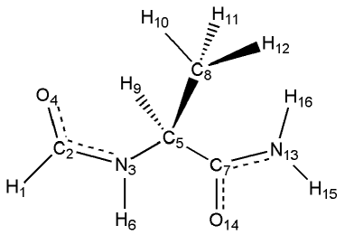
Figure 1: Atom numeration of the protected dipeptide HCO-L-Ala-NH₂.

The ab initio quantum mechanical calculations have been done with the package GAMESS [79] under Linux and in 3.20 GHz PIV machines. The coordinates used for the HCO-L-Ala-NH₂ dipeptide in the GAMESS input files and the ones used to generate them with automatic Perl scripts are the SASMIC coordinates introduced in ref. 59. They are presented in table 3 indicating the name of the conventional dihedral angles (see also fig. 1 for reference). To perform the energy optimizations, however, they have been converted to Delocalized Coordinates [80] in order to accelerate convergence.

Atom name	Bond length	Bond angle	Dihedral angle
H1
C2	(2,1)
N3	(3,2)	(3,2,1)
O4	(4,2)	(4,2,1)	(4,2,1,3)
C5	(5,3)	(5,3,2)	$\omega_{0}:=$(5,3,2,1)
H6	(6,3)	(6,3,2)	(6,3,2,5)
C7	(7,5)	(7,5,3)	$\phi:=$(7,5,3,2)
C8	(8,5)	(8,5,3)	(8,5,3,7)
H9	(9,5)	(9,5,3)	(9,5,3,7)
H10	(10,8)	(10,8,5)	$\chi:=$(10,8,5,3)
H11	(11,8)	(11,8,5)	(11,8,5,10)
H12	(12,8)	(12,8,5)	(12,8,5,10)
N13	(13,7)	(13,7,5)	$\psi:=$(13,7,5,3)
O14	(14,7)	(14,7,5)	(14,7,5,13)
H15	(15,13)	(15,13,7)	$\omega_{1}:=$(15,13,7,5)
H16	(16,13)	(16,13,7)	(16,13,7,15)

Table 3: SASMIC internal coordinates (Echenique P. and Alonso J. L., To be published in J. Comp. Chem., arXiv:q-bio.BM/0511004) in Z-matrix form of the protected dipeptide HCO-L-Ala-NH₂. Principal dihedrals are indicated in bold face and their typical biochemical name is given.

First, we have calculated the typical Potential Energy Surface (PES) in a regular 12x12 grid of the bidimensional space spanned by the Ramachandran angles $\phi$ and $\psi$, with both angles ranging from $-165^{o}$ to $165^{o}$ in steps of $30^{o}$. This has been done by running constrained energy optimizations at the MP2/6-31++G(d,p) level of the theory, freezing the two Ramachandran angles at each value of the grid, starting from geometries previously optimized at a lower level of the theory and setting the gradient convergence criterium to OPTTOL=$10^{-5}$ and the self-consistent Hartree-Fock convergence criterium to CONV=$10^{-6}$.

The results of these calculations (which took $\sim$ 100 days of CPU time) are 144 conformations that define $\Sigma$ and the values of $V_{\Sigma}(\phi,\psi)$ at these points (the PES itself).

Then, at each optimized point of $\Sigma$, we have calculated the Hessian matrix in the coordinates of table 3 removing the rows and columns corresponding to the soft angles $\phi$ and $\psi$, the result being the matrix $\mathcal{H}(\phi,\psi)$ in eq. 2.12b. This has been done, again, at the MP2/6-31++G(d,p) level of the theory, taking $\sim$ 140 days of CPU time.

Eqs. 3.2 and  3.7 in sec. 3.1 have been used to calculate the kinetic entropy terms associated to the determinants of the mass-metric tensors $G$ and $g$, respectively. The quantities in eq. 3.2, being simply internal coordinates, have been directly extracted from the GAMESS output files via automated Perl scripts. On the other hand, in order to calculate the matrix $g_{2}$ in eq. 3.4 that appears in the kinetic entropy of the classical rigid model, the Euclidean coordinates $\vec{x}_{\alpha}^{\,\prime}$ of the 16 atoms in the reference frame fixed in the system, as well as their derivatives with respect to $q^{i}\equiv(\phi,\psi)$, must be computed. For this, two additional 12x12 grids as the one described above have been computed; one of them displaced 2^o in the positive $\phi$-direction and the other one displaced 2^o in the positive $\psi$-direction. This has been done, again, at the MP2/6-31++G(d,p) level of the theory, starting from the optimized structures found in the computation of the PES described above and taking $\sim$ 75 days of CPU time each grid. Using the values of the positions $\vec{x}_{\alpha}^{\,\prime}$ in these two new grids and also in the original one, the derivatives of these quantities with respect to the angles $\phi$ and $\psi$, appearing in $g_{2}$, have been numerically obtained as finite differences.

The three calculations have been repeated for six special points in the Ramachandran space that correspond to important elements of secondary structure (see sec. 4), the total CPU time needed for computing all correcting terms at these points has been $\sim$ 16 days. A total of $\sim$ 406 days of CPU time has been needed to perform the whole study at the MP2/6-31++G(d,p) level of the theory.

Finally, we have repeated all the calculations at the HF/6-31++G(d,p) level of the theory in order to investigate if this less demanding method ($\sim$ 10 days for the PES, $\sim$ 8 days for the Hessians, $\sim$ 10 days for each displaced grid, $\sim$ 2 days for the special secondary structure points, being a total of $\sim$ 40 days of CPU time) may be used instead of MP2 in further studies.

4 Results

In table 4, the maximum variation, the average and the standard deviation in the 12x12 grid defined in the Ramachandran space of the protected dipeptide HCO-L-Ala-NH₂ are shown for the three energy surfaces, $V_{\Sigma}$, $F_{\mathrm{s}}$ and $F_{\mathrm{r}}$ (see eqs. 2.12 and 2.23), for the three correcting terms, $-TS_{\mathrm{s}}^{\mathrm{k}}$, $-TS_{\mathrm{s}}^{\mathrm{c}}$, and $-TS_{\mathrm{r}}^{\mathrm{k}}$ and for the Fixman’s compensating potential $V_{\mathrm{F}}$ (see eq. 2.25). All the functions have been referenced to zero in the grid.

	MP2/6-31++G(d,p)			HF/6-31++G(d,p)
	Max.a	Ave.b	Std.c	Max.a	Ave.b	Std.c
$V_{\Sigma}$	21.64	6.76	3.88	23.62	6.92	4.35
$F_{\mathrm{s}}$	21.43	6.47	3.93	23.78	7.17	4.38
$F_{\mathrm{r}}$	21.09	6.46	3.82	23.09	6.76	4.31
$-TS_{\mathrm{s}}^{\mathrm{k}}$	0.24	0.09	0.05	0.23	0.09	0.04
$-TS_{\mathrm{s}}^{\mathrm{c}}$	1.67	0.98	0.32	1.34	0.63	0.30
$-TS_{\mathrm{r}}^{\mathrm{k}}$	0.81	0.37	0.12	0.75	0.38	0.12
$V_{\mathrm{F}}$	1.68	0.89	0.30	1.35	0.55	0.27

Table 4: ^aMaximum variation, ^baverage and ^cstandard deviation in the 12x12 grid defined in the Ramachandran space of the protected dipeptide HCO-L-Ala-NH₂ for the three energy surfaces, $V_{\Sigma}$, $F_{\mathrm{s}}$ and $F_{\mathrm{r}}$, the three correcting terms, $-TS_{\mathrm{s}}^{\mathrm{k}}$, $-TS_{\mathrm{s}}^{\mathrm{c}}$, and $-TS_{\mathrm{r}}^{\mathrm{k}}$ and the Fixman’s compensating potential $V_{\mathrm{F}}$. The results at both MP2/6-31++G(d,p) and HF/6-31++G(d,p) levels of the theory are presented and all the functions have been referenced to zero in the grid. The units used are kcal/mol.

In fig. 2, the Potential Energy Surface $V_{\Sigma}$, at the MP2/6-31++G(d,p) level of the theory, is depicted with the reference set to zero for visual convenience. Neither the surfaces defined by $F_{\mathrm{s}}$ and $F_{\mathrm{r}}$ at the MP2/6-31++G(d,p) level of the theory nor the three energy surfaces $V_{\Sigma}$, $F_{\mathrm{s}}$ and $F_{\mathrm{r}}$ at HF/6-31++G(d,p) are shown graphically since they are visually very similar to the surface in fig. 2.

In fig. 3, the three correcting terms, $-TS_{\mathrm{s}}^{\mathrm{k}}$, $-TS_{\mathrm{s}}^{\mathrm{c}}$ and $-TS_{\mathrm{r}}^{\mathrm{k}}$ and the Fixman’s compensating potential $V_{\mathrm{F}}$, at the MP2/6-31++G(d,p) level of the theory, are depicted with the reference set to zero. The analogous surfaces at the HF/6-31++G(d,p) level of the theory are visually very similar to the ones in fig. 3 and have been therefore omitted.

Figure 2: Potential Energy Surface (PES) of the model dipeptide HCO-L-Ala-NH₂, computed at the MP2/6-31++G(d,p) level of the theory. The surface has been referenced to zero and smoothed with bicubic splines for visual convenience. The units in the z-axis are kcal/mol.

From the results presented, one may conclude that, although the conformational dependence of the correcting terms $-TS_{\mathrm{s}}^{\mathrm{k}}$, $-TS_{\mathrm{s}}^{\mathrm{c}}$ and $-TS_{\mathrm{r}}^{\mathrm{k}}$ is more than an order of magnitude smaller than the conformational dependence of the Potential Energy Surface $V_{\Sigma}$ in the worst case, if chemical accuracy (typically defined in the field of ab initio quantum chemistry as $1$ kcal/mol [81]) is sought, they may be relevant. In fact, they are of the order of magnitude of the differences between the energy surfaces $V_{\Sigma}$, $F_{\mathrm{s}}$ and $F_{\mathrm{r}}$ calculated at MP2/6-31++G(d,p) and the ones calculated at HF/6-31++G(d,p).

For the same reasons, we may conclude that, if ab initio derived potentials are used to carry out Molecular Dynamics simulations of peptides, the Fixman’s compensating potential $V_{\mathrm{F}}$ should be included. Finally, regarding the relative importance of the different correcting terms $-TS_{\mathrm{s}}^{\mathrm{k}}$, $-TS_{\mathrm{s}}^{\mathrm{c}}$ and $-TS_{\mathrm{r}}^{\mathrm{k}}$, the results in table 4 suggest that the less important one is the kinetic entropy $-TS_{\mathrm{s}}^{\mathrm{k}}$ of the stiff case (related to the determinant of the mass-metric tensor $G$) and that the most important one is the one related to the determinant of the Hessian matrix $\mathcal{H}$ of the constraining part of the potential, i.e., the conformational entropy $-TS_{\mathrm{s}}^{\mathrm{k}}$. The first conclusion is in agreement with the approximations typically made in the literature, the second one, however, is not (see the Appendix).

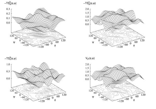
Figure 3: Ramachandran plots of the correcting terms appearing in eqs. 2.12 and 2.23, together with the Fixman’s compensating potential defined in eq. 2.25, computed at the MP2/6-31++G(d,p) level of the theory in the model dipeptide HCO-L-Ala-NH₂. The surfaces have been referenced to zero and smoothed with bicubic splines for visual convenience. The units in the z-axes are kcal/mol.

Now, although the relative sizes of the conformational dependence of the different terms may be indicative of their importance, the degree of correlation among the surfaces is also relevant (see table 6). Hence, in order to arrive to more precise conclusions, we reexamine here the results using a physically meaningful criterium to compare potential energy functions that has been introduced in ref. 82. The distance, denoted by $d_{12}$, between any two different potential energy functions, $V_{1}$ and $V_{2}$, is an statistical quantity that, from a working set of conformations (in this case, the 144 points of the grid), measures the typical error that one makes in the energy differences if $V_{2}$ is used instead of $V_{1}$, admitting a linear rescaling.

Corr.a	${V_{1}}^{b}$	${V_{2}}^{c}$	${d_{12}}^{d}$	${N_{\mathrm{res}}}^{e}$	${b_{12}}^{f}$	${r_{12}}^{g}$
MP2/6-31++G(d,p)
$-TS_{\mathrm{s}}^{\mathrm{k}}-TS_{\mathrm{s}}^{\mathrm{c}}$	$F_{\mathrm{s}}$	$V_{\Sigma}$	0.74 $RT$	1.82	0.98	0.9967
$-TS_{\mathrm{s}}^{\mathrm{c}}$	$F_{\mathrm{s}}$	$V_{\Sigma}-TS_{\mathrm{s}}^{\mathrm{k}}$	0.74 $RT$	1.83	0.98	0.9967
$-TS_{\mathrm{s}}^{\mathrm{k}}$	$F_{\mathrm{s}}$	$V_{\Sigma}-TS_{\mathrm{s}}^{\mathrm{c}}$	0.11 $RT$	80.45	1.00	0.9999
$-TS_{\mathrm{r}}^{\mathrm{k}}$	$F_{\mathrm{r}}$	$V_{\Sigma}$	0.29 $RT$	11.62	1.01	0.9995
$V_{\mathrm{F}}$	$F_{\mathrm{s}}$	$F_{\mathrm{r}}$	0.67 $RT$	2.24	0.97	0.9972
HF/6-31++G(d,p)
$-TS_{\mathrm{s}}^{\mathrm{k}}-TS_{\mathrm{s}}^{\mathrm{c}}$	$F_{\mathrm{s}}$	$V_{\Sigma}$	0.73 $RT$	1.90	0.99	0.9975
$-TS_{\mathrm{s}}^{\mathrm{c}}$	$F_{\mathrm{s}}$	$V_{\Sigma}-TS_{\mathrm{s}}^{\mathrm{k}}$	0.71 $RT$	2.00	0.99	0.9976
$-TS_{\mathrm{s}}^{\mathrm{k}}$	$F_{\mathrm{s}}$	$V_{\Sigma}-TS_{\mathrm{s}}^{\mathrm{c}}$	0.10 $RT$	90.99	1.00	0.9999
$-TS_{\mathrm{r}}^{\mathrm{k}}$	$F_{\mathrm{r}}$	$V_{\Sigma}$	0.26 $RT$	14.83	1.01	0.9997
$V_{\mathrm{F}}$	$F_{\mathrm{s}}$	$F_{\mathrm{r}}$	0.61 $RT$	2.69	0.98	0.9982
MP2/6-31++G(d,p) vs. HF/6-31++G(d,p)
	$V_{\Sigma}$	$V_{\Sigma}$	1.25 $RT$	0.64	1.12	0.9925
	$F_{\mathrm{s}}$	$F_{\mathrm{s}}$	1.18 $RT$	0.72	1.11	0.9934
	$F_{\mathrm{r}}$	$F_{\mathrm{r}}$	1.18 $RT$	0.72	1.12	0.9932

Table 5: Comparison of different energy surfaces involved in the study of the constrained equilibrium of the protected dipeptide HCO-L-Ala-NH₂. ^aCorrecting term whose importance is measured in the corresponding row, ^breference potential energy $V_{1}$ (the “correct” one, the one containing the correcting term), ^capproximated potential energy $V_{2}$ (i.e, $V_{1}$ minus the correcting term in column $a$), ^dstatistical distance between $V_{1}$ and $V_{2}$ (see Alonso J. L. and Echenique P., J. Comp. Chem. 27 (2006) 238–252), ^emaximum number of residues in a polypeptide potential up to which the correcting term in column $a$ may be omitted, ^fslope of the linear rescaling between $V_{1}$ and $V_{2}$ and ^gPearson’s correlation coefficient. All quantities are dimensionless, except for $d_{12}$ which is given in units of the thermal energy $RT$ at $300^{o}$ K.

In table 5, which contains the central results of this work, the distances between some of the energy surfaces that play a role in the problem are shown. We present the result in units of $RT$ (at $300^{o}$ K, where $RT\simeq 0.6$ kcal/mol) because it has been argued in ref. 82 that, if the distance between two different approximations of the energy of the same system is less than $RT$, one may safely substitute one by the other without altering the relevant physical properties. Moreover, if one assumes that the effective energies compared will be used to construct a polypeptide potential and that it will be designed as simply the sum of mono-residue ones (making each term suitably depend on different pairs of Ramachandran angles), then, the number $N_{\mathrm{res}}$ of residues up to which one may go keeping the distance between the two approximations of the the $N$-residue potential below $RT$ is (see eq. 23 in ref. 82):

$$N_{\mathrm{res}}=\left(\frac{RT}{d_{12}}\right)^{2}\ .$$ (4.1)

This number is also shown in table 5, together with the slope $b_{12}$ of the linear rescaling between $V_{1}$ and $V_{2}$ and the Pearson’s correlation coefficient [83], denoted by $r_{12}$.

${V_{1}}^{a}$		${V_{2}}^{b}$	${r_{12}}^{c}$
MP2/6-31++G(d,p)
$V_{\Sigma}$	vs.	$-TS_{\mathrm{s}}^{\mathrm{c}}$	0.1572
$V_{\Sigma}$	vs.	$-TS_{\mathrm{s}}^{\mathrm{k}}$	-0.0008
$V_{\Sigma}$	vs.	$-TS_{\mathrm{r}}^{\mathrm{k}}$	-0.3831
$V_{\Sigma}$	vs.	$V_{\mathrm{F}}$	0.3334
HF/6-31++G(d,p)
$V_{\Sigma}$	vs.	$-TS_{\mathrm{s}}^{\mathrm{c}}$	0.0682
$V_{\Sigma}$	vs.	$-TS_{\mathrm{s}}^{\mathrm{k}}$	0.0897
$V_{\Sigma}$	vs.	$-TS_{\mathrm{r}}^{\mathrm{k}}$	-0.3544
$V_{\Sigma}$	vs.	$V_{\mathrm{F}}$	0.2404
MP2/6-31++G(d,p) vs. HF/6-31++G(d,p)
$-TS_{\mathrm{s}}^{\mathrm{c}}$	vs.	$-TS_{\mathrm{s}}^{\mathrm{c}}$	0.9136
$-TS_{\mathrm{s}}^{\mathrm{k}}$	vs.	$-TS_{\mathrm{s}}^{\mathrm{k}}$	0.9808
$-TS_{\mathrm{r}}^{\mathrm{k}}$	vs.	$-TS_{\mathrm{r}}^{\mathrm{k}}$	0.9316
$V_{\mathrm{F}}$	vs.	$V_{\mathrm{F}}$	0.9217

Table 6: Correlation between the different correcting terms involved in the study of the constrained equilibrium of the protected dipeptide HCO-L-Ala-NH₂. ^aReference potential energy, ^bapproximated potential energy, ^cPearson’s correlation coefficient.

The results at both MP2/6-31++G(d,p) and HF/6-31++G(d,p) levels of the theory are presented. The first three rows in each of the first two blocks are related to the classical stiff model, the next row to the classical rigid model and the last one in each block to the comparison between the two models. The third block in the table is associated to the comparison between the two different levels of the theory used.

The $F_{\mathrm{s}}$ vs. $V_{\Sigma}$ row (in the first two blocks) assess the importance of the two correcting terms, $-TS_{\mathrm{s}}^{\mathrm{k}}$ and $-TS_{\mathrm{s}}^{\mathrm{c}}$, in the stiff case. The result $d_{12}=0.74RT$ indicates that, for the alanine dipeptide, $V_{\Sigma}$ may be used as an approximation of $F_{\mathrm{s}}$ with caution if accurate results are sought. In fact, the low value of $N_{\mathrm{res}}=1.82<2$ shows that, if we wanted to describe a 2-residue peptide omitting the stiff correcting terms, we would typically make an error greater than the thermal noise in the energy differences. The next two rows investigate the effect of each one of the individual correcting terms. The conclusion that can be extracted from them (as the relative sizes in table 4 already suggested) is that the conformational entropy associated to the determinant of the Hessian matrix $\mathcal{H}$ is much more relevant than the correcting term $-TS_{\mathrm{s}}^{\mathrm{k}}$, related to the mass-metric tensor $G$, allowing to drop the latter up to $\sim 80$ residues (according to MP2/6-31++G(d,p) calculations). As has been already remarked, this second conclusion is in agreement with the approximations frequently done in the literature; however, it turns out that the importance of the Hessian-related term has been persistently underestimated (see the Appendix for a discussion).

The $F_{\mathrm{r}}$ vs. $V_{\Sigma}$ row, in turn, shows the data associated to the kinetic entropy term $-TS_{\mathrm{r}}^{\mathrm{k}}$, which is related to the determinant of the reduced mass-metric tensor $g$ in the classical rigid model. From the results there ($d_{12}=0.29RT$ and $N_{\mathrm{res}}=11.62$ at the MP2/6-31++G(d,p) level), we can conclude that the only correction term in the rigid case is less important than the ones in the stiff case and that $V_{\Sigma}$ may be used as an approximation of $F_{\mathrm{r}}$ for oligopeptides of up to $\sim 12$ residues.

The last row in each of the first two blocks in table 5 is related to the interesting question in Molecular Dynamics of whether or not one should include the Fixman’s compensating potential $V_{F}$ (see eq. 2.25) in rigid simulations in order to obtain the stiff equilibrium distribution, $\exp(-\beta F_{\mathrm{s}})$, instead of the rigid one, $\exp(-\beta F_{\mathrm{r}})$. This question is equivalent to asking whether or not $F_{\mathrm{r}}$ is a good approximation of $F_{\mathrm{s}}$. From the results in the table, we can conclude that the Fixman’s potential is relevant for peptides of more than 2 residues and its omission may cause an error greater than the thermal noise in the energy differences.

The appreciable sizes of the different correcting terms, shown in table 4, together with their low correlation with the Potential Energy Surface $V_{\Sigma}$, presented in the first two blocks of table 6, explain their considerable relevance discussed in the preceding paragraphs.

Moreover, from the comparison of the MP2/6-31++G(d,p) and the HF/6-31++G(d,p) blocks, one can tell that the study herein performed may well have been done at the lower level of the theory (if we had known) with a tenth of the computational effort (see sec. 3). This fact, explained by the high correlation, presented in the third block of table 6, between the correcting terms calculated at the two levels, is very relevant for further studies on more complicated dipeptides or longer chains and it indicates that the differences in size between the different correcting terms at MP2/6-31++G(d,p) and HF/6-31++G(d,p), which are presented in table 4, are mostly due to a harmless linear scaling effect similar to the well-known empirical scale factor frequently used in ab initio vibrational analysis [84, 85, 86]. This view is supported by the data in the third block of table 5, related to the comparison between the energy surfaces calculated at MP2/6-31++G(d,p) and HF/6-31++G(d,p), where the slopes $b_{12}$ are consistently larger than unity.

A last conclusion that may be extracted from the block labeled “MP2/6-31++G(d,p) vs. HF/6-31++G(d,p)” in table 5 is that the typical error in the energy differences (given by the distances $d_{12}$) produced when one reduces the level of the theory from MP2/6-31++G(d,p) to HF/6-31++G(d,p) is comparable (less than twice) to the error made if the most important correcting terms of the classical constrained models studied in this work are dropped. This is a useful hint for researchers interested in the conformational analysis of peptides with quantum chemistry methods [60, 61, 62, 87, 63, 64, 70] and also to those whose aim is the design and parametrization of classical force fields from ab initio quantum mechanical calculations [68, 69, 70].

	$\phi$	$\psi$
$\alpha$-helix	-57	-47
310-helix	-49	-26
$\pi$-helix	-57	-70
polyproline II	-79	149
parallel $\beta$-sheet	-119	113
antiparallel $\beta$-sheet	-139	135

Table 7: Ramachandran angles (in degrees) of some important secondary structure elements in polypeptides. Data taken from Lesk A. M., Introduction to Protein Architecture, Oxford University Press, Oxford, 2001.

Finally, in order to enrich and qualify the analysis, a new working set of conformations, different from the 144 points of the grid in the Ramachandran space, have been selected and the whole study has been repeated on them. These new conformations are six important secondary structure elements which form repetitive patterns stabilized by hydrogen bonds in polypeptides. Their conventional names and the corresponding values of the $\phi$ and $\psi$ angles have been taken from ref. 88 and are shown in table 7.

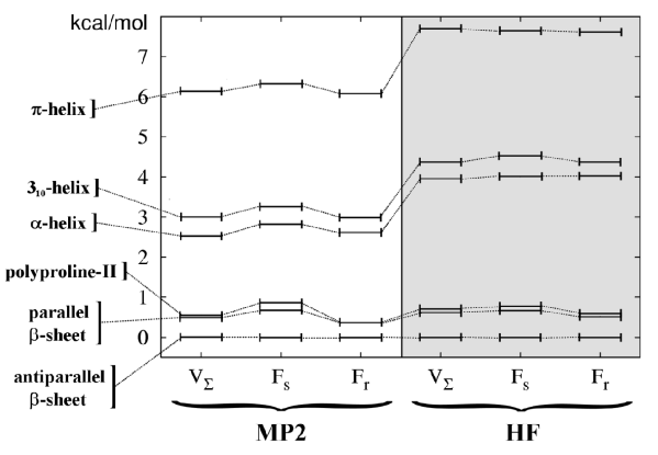
Figure 4: Relative energies of some important elements of secondary structure for the three potentials $V_{\Sigma}$, $F_{\mathrm{s}}$ and $F_{\mathrm{r}}$, in the model dipeptide HCO-L-Ala-NH₂ and at both MP2/6-31++G(d,p) and HF/6-31++G(d,p) levels of the theory. The energy of the antiparallel $\beta$-sheet has been taken as reference. The units are kcal/mol.

In fig. 4, the relative energies of these conformations are shown for the three relevant potentials, $V_{\Sigma}$, $F_{\mathrm{s}}$ and $F_{\mathrm{r}}$, at both MP2/6-31++G(d,p) and HF/6-31++G(d,p) levels of the theory. Since the antiparallel $\beta$-sheet is the structure with the minimum energy in all the cases, it has been set as the reference and the rest of energies in the figure should be regarded as relative to it.

The meaningful assessment, using the statistical distance described above, of the typical error made in the energy differences has been also performed on this new working set of conformations. The results are presented in table 8.

Corr.a	${V_{1}}^{b}$	${V_{2}}^{c}$	${d_{12}}^{d}$	${N_{\mathrm{res}}}^{e}$	${b_{12}}^{f}$	${r_{12}}^{g}$
MP2/6-31++G(d,p)
$-TS_{\mathrm{s}}^{\mathrm{k}}-TS_{\mathrm{s}}^{\mathrm{c}}$	$F_{\mathrm{s}}$	$V_{\Sigma}$	0.22 $RT$	19.72	0.99	0.9990
$-TS_{\mathrm{s}}^{\mathrm{c}}$	$F_{\mathrm{s}}$	$V_{\Sigma}-TS_{\mathrm{s}}^{\mathrm{k}}$	0.26 $RT$	14.07	0.98	0.9985
$-TS_{\mathrm{s}}^{\mathrm{k}}$	$F_{\mathrm{s}}$	$V_{\Sigma}-TS_{\mathrm{s}}^{\mathrm{c}}$	0.06 $RT$	298.13	1.01	0.9999
$-TS_{\mathrm{r}}^{\mathrm{k}}$	$F_{\mathrm{r}}$	$V_{\Sigma}$	0.20 $RT$	25.64	0.99	0.9992
$V_{\mathrm{F}}$	$F_{\mathrm{s}}$	$F_{\mathrm{r}}$	0.34 $RT$	8.73	0.99	0.9977
HF/6-31++G(d,p)
$-TS_{\mathrm{s}}^{\mathrm{k}}-TS_{\mathrm{s}}^{\mathrm{c}}$	$F_{\mathrm{s}}$	$V_{\Sigma}$	0.14 $RT$	47.94	1.00	0.9997
$-TS_{\mathrm{s}}^{\mathrm{c}}$	$F_{\mathrm{s}}$	$V_{\Sigma}-TS_{\mathrm{s}}^{\mathrm{k}}$	0.15 $RT$	46.12	1.00	0.9997
$-TS_{\mathrm{s}}^{\mathrm{k}}$	$F_{\mathrm{s}}$	$V_{\Sigma}-TS_{\mathrm{s}}^{\mathrm{c}}$	0.05 $RT$	380.30	1.00	0.9999
$-TS_{\mathrm{r}}^{\mathrm{k}}$	$F_{\mathrm{r}}$	$V_{\Sigma}$	0.15 $RT$	41.85	0.99	0.9997
$V_{\mathrm{F}}$	$F_{\mathrm{s}}$	$F_{\mathrm{r}}$	0.18 $RT$	30.12	1.01	0.9996
MP2/6-31++G(d,p) vs. HF/6-31++G(d,p)
	$V_{\Sigma}$	$V_{\Sigma}$	0.77 $RT$	1.68	1.28	0.9929
	$F_{\mathrm{s}}$	$F_{\mathrm{s}}$	0.77 $RT$	1.69	1.26	0.9928
	$F_{\mathrm{r}}$	$F_{\mathrm{r}}$	0.71 $RT$	1.96	1.28	0.9939

Table 8: Comparison of different approximations to the energies of some important elements of secondary structure (see table 7) in the study of the constrained equilibrium of the protected dipeptide HCO-L-Ala-NH₂. See the caption of table 5 for an explanation of the keys in the different columns.

The distances between the free energies, $F_{\mathrm{s}}$ and $F_{\mathrm{r}}$, and their corresponding approximations obtained dropping the correcting entropies, $-TS_{\mathrm{s}}^{\mathrm{k}}$, $-TS_{\mathrm{s}}^{\mathrm{c}}$ and $-TS_{\mathrm{r}}^{\mathrm{k}}$, or the Fixman’s compensating potential $V_{\mathrm{F}}$, in the first two blocks of the table, are consistently smaller than the ones found in the study of the grid defined in the whole Ramachandran space (cf. table 5). And so are the distances between the three relevant potentials, $V_{\Sigma}$, $F_{\mathrm{s}}$ and $F_{\mathrm{r}}$, calculated at the MP2/6-31++G(d,p) and HF/6-31++G(d,p) levels of the theory.

Although the distance $d_{12}$ used is a statistical quantity and, therefore, one must be cautious when working with such a small set of conformations (of size six, in this case), the conclusion drawn from this second part of the study is that, if one is interested only in the “lower region” of the Ramachandran surface, where the typical secondary structure elements lie, then, one may safely neglect the conformational dependence of the different correcting terms appearing in the study of the constrained equilibrium of peptides. At least, up to oligopeptides (poly-alanines) of $\sim$ 10 residues in the worst case (the neglect of the Fixman’s compensating potential $V_{\mathrm{F}}$ in the $F_{\mathrm{s}}$ vs. $F_{\mathrm{r}}$ comparison at MP2/6-31++G(d,p)).

This difference between the two working set of conformations may be explained looking at one of the ways of expressing the statistical distance used (see eq. 12a in ref. 82):

$$d_{12}=\sqrt{2}\,{\sigma}_{2}(1-r_{12}^{2})^{1/2}\ ,$$ (4.2)

where $r_{12}$ is the Pearson’s correlation coefficient between the potential energies denoted by $V_{1}$ and $V_{2}$ and ${\sigma}_{2}$ is the standard deviation in the values of $V_{2}$ on the relevant working set of conformations.

This last quantity, ${\sigma}_{2}$, is the responsible of the differences between tables 5 and 8, since the set of conformations comprised by the six secondary structure elements in table 7 spans a smaller energy range than the whole Potential Energy Surface in fig. 2 (or $F_{\mathrm{s}}$, or $F_{\mathrm{r}}$, which have very similar variations). Accordingly, the dispersion in the energy values is smaller: $\sigma_{2}\simeq$ 2 kcal/mol in the case of the secondary structure elements and $\sigma_{2}\simeq$ 4 kcal/mol for the grid in the whole Ramachandran space (see table 4). Since the correlation coefficient in both cases are of similar magnitude, the differences in $\sigma_{2}$ produce a smaller distance $d_{12}$ for the second set of conformations studied, i.e., a smaller typical error made in the energy differences when omitting the correcting terms derived from the consideration of constraints.

To end this section, we remark that, although this “lower region” of the Ramachandran space contains the most relevant secondary structure elements (which are also the most commonly found in experimentally resolved native structures of proteins [89, 90, 91, 92]) and may be the only region explored in the dynamical or thermodynamical study of small peptides, if the aim is the design of effective potentials for computer simulation of polypeptides [68, 69, 70], then, some caution is recommended, since long-range interactions in the sequence may temporarily compensate local energy penalizations and the higher regions of the energy surfaces studied could be important in transition states or in some relevant dynamical paths of the system.

In the following section, the many results discussed in the preceding paragraphs are summarized.

5 Conclusions

In this work, the theory of classical constrained equilibrium has been collected for the stiff and rigid models. The pertinent correcting terms, which may be regarded as effective entropies, as well as the Fixman’s compensating potential, have been derived and theoretically discussed (see eqs. 2.12, 2.23 and 2.25, together with the formulae in sec. 3.1). In addition, the common approximation of considering that, for typical internals, the equilibrium values of the hard coordinates do not depend on the soft ones, has also been discussed and related to the rest of simplifications. The treatment of the assumptions in the literature is thoroughly reviewed and discussed in the Appendix.

In the central part of the work (sec. 4), the relevance of the different correcting terms has been assessed in the case of the model dipeptide HCO-L-Ala-NH₂, with quantum mechanical calculations including electron correlation. Also, the possibility of performing analogous studies at the less demanding Hartree-Fock level of the the theory has been investigated. The results found are summarized in the following points:

• In Monte Carlo simulations of the classical stiff model at room temperature, the effective entropy $-TS_{\mathrm{s}}^{\mathrm{k}}$, associated to the determinant of the mass-metric tensor $G$, may be neglected for peptides of up to $\sim$ 80 residues. Its maximum variation in the Ramachandran space is 0.24 kcal/mol.

• In Monte Carlo simulations of the classical stiff model at room temperature, the effective entropy $-TS_{\mathrm{s}}^{\mathrm{c}}$, associated to the determinant of the Hessian $\mathcal{H}$ of the constraining part of the potential, should be included for peptides of more than 2 residues. Its maximum variation in the Ramachandran space is 1.67 kcal/mol.

• In Monte Carlo simulations of the classical rigid model at room temperature, the effective entropy $-TS_{\mathrm{r}}^{\mathrm{k}}$, associated to the determinant of the reduced mass-metric tensor $g$, may be neglected for peptides of up to $\sim$ 12 residues. Its maximum variation in the Ramachandran space is 0.81 kcal/mol.

• In rigid Molecular Dynamics simulations intended to yield the stiff equilibrium distribution at room temperature, the Fixman’s compensating potential $V_{\mathrm{F}}$ should be included for peptides of more than 2 residues. Its maximum variation in the Ramachandran space is 1.68 kcal/mol.

• If the assumption that only the more stable region of the Ramachandran space, where the principal elements of secondary structure lie, is relevant, then, the importance of the correcting terms decreases and the limiting number of residues in a polypeptide potential up to which they may be omitted is approximately four times larger in each of the previous points.

• In both cases (i.e., either if the whole Ramachandran space is considered relevant, or only the lower region), the errors made if the most important correcting terms are neglected are of the same order of magnitude as the errors due to a decrease in the level of theory from MP2/6-31++G(d,p) to HF/6-31++G(d,p).

• The whole study of the relevance of the different correcting terms (or future analogous investigations) may be performed at the HF/6-31++G(d,p) level of the theory, yielding very similar results to the ones obtained at MP2/6-31++G(d,p) and using a tenth of the computational effort.

To end this discussion, some qualifications should be made. On one hand, the conclusions above refer to the case in which a classical potential directly extracted from the quantum mechanical (Born-Oppenheimer) one is used; for the considerably simpler force fields typically used for macromolecular simulations, the study should be repeated and different results may be obtained. On the other hand, the investigation performed in this work has been done in one of the simplest dipeptides; both its isolated character and the relatively small size of its side chain play a role in the results obtained. Hence, for bulkier residues included in polypeptides, these conclusions should be approached with caution and much interesting work remains to be done.

Appendix

Many approximations may be done to simplify the calculation of the different correcting terms introduced in the previous subsections. The most frequently found in the literature are the following three:

1. To neglect the conformational dependence of $\det G$.

2. To neglect the conformational dependence of $\det\mathcal{H}$.

3. To assume that the hard coordinates are constant, i.e, that the $f^{I}(q^{i})$ in eq. 2.1 do not depend on the soft coordinates $q^{i}$.

The conformational dependence of $\det g$ is customarily regarded as important since it was shown to be non-negligible even for simple systems some decades ago [21, 22, 13, 23] (normally in an indirect way, while studying the influence of the Fixman’s compensating potential in eq. 2.25; see discussion below). With this same aim, Patriciu et al. [20] have very recently measured the conformational dependence of $\det g$ for a serial polymer with fixed bond lengths and bond angles (in the approximation (iii)), showing that it is non-negligible and suggesting that it may be so also for more general systems.

Note that, if approximations (i) and (ii) are assumed, then the Fixman’s potential depends only on $\det g$. In fact, whereas in the general case the Fixman’s compensating potential cannot be simplified beyond the expression in eq. 2.25, if one assumes approximation (iii), then the reduced mass-metric tensor $g$ turns out to be the subblock of $G$ with soft indices and, in this case, the quotient $\det G/\det g$ has been shown to be equal to $1/\det h$ by Fixman [16], where $h$ denotes the subblock of $G^{-1}$ with hard indices, i.e.,

$$h^{IJ}(q^{\mu}):=\sum_{\sigma=1}^{N}\frac{\partial q^{I}}{\partial x^{\sigma}}\frac{1}{m_{\sigma}}\frac{\partial q^{J}}{\partial x^{\sigma}}\ .$$ (5.1)

This result has been extensively used in the literature [38, 57, 21, 22, 23, 42], since each of the internal coordinates $q^{a}$ typically used in macromolecular simulations only involves a small number of atoms, thus rendering the matrix $h$ above sparse and allowing for efficient algorithms to be used in order to find its determinant.

Now, although $\det g$ is customarily regarded as important, the conformational variations of $\det G$ are almost unanimously neglected (approximation (i)) in the literature [55, 15] and may only be said to be indirectly included in $h$ by the authors that use the expression above [20, 38, 57, 21, 22, 23]. This is mainly due to the fact, reported by Gō and Scheraga [15] and, before, by Volkenstein [74], that $\det G$ in a serial polymer may be expressed as in eq. 3.1, being independent of the dihedral angles (which are customarily taken as the soft coordinates). If one also assumes approximation (iii), which, as will be discussed later, is very common, then $\det G$ is a constant for every conformation of the molecule.

Probably due to computational considerations, but also sometimes to the use of a formulation of the stiff case based on delta functions [51], the conformational dependence of $\det\mathcal{H}$ is almost unanimously neglected (approximation (ii)) in the literature [65, 20, 66, 19, 55, 41, 15, 16]. Only a few authors include this term in different stages of the reasoning [18, 19, 39, 26, 13, 14, 15], most of them only to argue later that it is negligible.

Although for some simple ad hoc designed potentials that lack long-range terms [57, 21, 22], the aforementioned simplifying assumptions and the ones that will be discussed in the following paragraphs may be exactly fulfilled, in the case of the potential energies used in force fields for macromolecular simulation [27, 28, 6, 29, 30, 31, 32, 33, 34, 35, 36, 37], they are not. The typical energy function in this case, has the form

$$V_{\mathrm{ff}}(q^{a}) := \frac{1}{2}\sum_{\alpha=1}^{N_{r}}K_{r_{\alpha}}(r_{\alpha}-r_{\alpha}^{0})^{2}+\frac{1}{2}\sum_{\alpha=1}^{N_{\theta}}K_{\theta_{\alpha}}(\theta_{\alpha}-\theta_{\alpha}^{\,0})^{2}+$$ (5.2)

$$+ V_{\mathrm{ff}}^{\mathrm{tors}}(\phi_{\alpha})+V_{\mathrm{ff}}^{\mathrm{long-range}}(q^{a})\ ,$$

where $r_{\alpha}$ are bond lengths, $\theta_{\alpha}$ are bond angles, $\phi_{\alpha}$ are dihedral angles and, for the sake of simplicity, no harmonic terms have been assumed for out-of-plane angles or for hard dihedrals (such as the peptide bond $\omega$). $N_{r}$ is the number of bond lengths, $N_{\theta}$ the number of bond angles and the quantities $K_{r_{\alpha}}$, $K_{\theta_{\alpha}}$, $r_{\alpha}^{0}$ and $\theta_{\alpha}^{\,0}$ are constants. The term denoted by $V_{\mathrm{ff}}^{\mathrm{tors}}(\phi_{\alpha})$ is a commonly included torsional potential that depends only on the dihedral angles $\phi_{\alpha}$ and $V_{\mathrm{ff}}^{\mathrm{long-range}}(q^{a})$ normally comprises long-range interactions such as Coulomb or van der Waals; hence, it depends on the atomic positions $\vec{x}_{\alpha}^{\,\prime}$ which, in turn, depend on all the internal coordinates $q^{a}$.

One of the reasons given for neglecting $\det\mathcal{H}$, when classical force fields are used with potential energy functions such as the one in eq. 5.2, is that the harmonic constraining terms dominate over the rest of interactions and, since the constants appearing on these terms (the $K_{r_{\alpha}}$, $K_{\theta_{\alpha}}$ in eq. 5.2) are independent of the conformation by construction, so is $\det\mathcal{H}$ [19, 26, 15]. Here, we analyze a more realistic quantum-mechanical potential and these considerations are not applicable, however, they also should be checked in the case of classical force fields, since, for a potential energy such as the one in eq. 5.2), the quantities $K_{r_{\alpha}}$ and $K_{\theta_{\alpha}}$ are finite and the long-range terms will also affect the Hessian at each point of the constrained hypersurface $\Sigma$, rendering its determinant conformation-dependent.

For the same reason, even in classical force fields, the equilibrium values of the hard coordinates are not the constant quantities $r_{\alpha}^{0}$ and $\theta_{\alpha}^{\,0}$ in eq. 5.2 but some functions $f^{I}(q^{i})$ of the soft coordinates (see eq. 2.1). This fact, recognized by some authors [93, 45, 25, 15], provokes that, if one chooses to assume approximation (iii) and the constants $r_{\alpha}^{0}$ and $\theta_{\alpha}^{\,0}$ appearing in eq. 5.2 are designated as the equilibrium values, the potential energy in $\Sigma$ may be heavily distorted, the cause being simply that the long-range interactions between atoms separated by three covalent bonds are not fully relaxed [93]. This effect is probably larger if bond angles, and not only bond lengths, are also constrained, which may partially explain the different dynamical behaviour found in ref. 6 when comparing these types of constraints in Molecular Dynamics simulations. In quantum mechanical calculations of small dipeptides, on the other hand, the fact that the bond lengths and bond angles depend on the Ramachandran angles $(\phi,\psi)$ has been pointed out by Schäffer et al. [94]. Therefore, approximation (iii), which is very common in the literature [65, 18, 20, 51, 38, 66, 19, 39, 95, 96, 55, 52, 40, 41, 26, 6, 13, 42, 15, 16], should be critically analyzed in each particular case.

Apart from the typical internal coordinates $q^{a}$ used until now, in terms of which the constrained hypersurface $\Sigma$ is described by the relations $q^{I}=f^{I}(q^{i})$ in eq. 2.1, with $I=M+7,\ldots,N$, one may define a different set $Q^{a}$ such that, on $\Sigma$, the corresponding hard coordinates are arbitrary constants $Q^{I}=C^{I}$ (the external coordinates $q^{A}$ and $Q^{A}$ are irrelevant for this part of the discussion). To do this, for example, let

$$\begin{array}[]{lll}Q^{i}:=q^{i}&i=7,\ldots,M+6&\mathrm{and}\\ Q^{I}:=q^{I}-f^{I}(q^{i})+C^{I}&I=M+7,\ldots,N\ .&\end{array}$$ (5.3)

Well then, while the relation between bond lengths, bond angles and dihedral angles (the typical $q^{a}$ [59]) and the Euclidean coordinates is straightforward and simple, the expression of the transformation functions $Q^{a}(x^{\mu})$ needs the knowledge of the $f^{I}$, which must be calculated numerically in most real cases. This drastically reduce the practical use of the $Q^{a}$, however, it is also true that they are conceptually appealing, since they have a property that closely match our intuition about what the soft and hard coordinates should be (namely, that the hard coordinates $Q^{I}$ are constant on the relevant hypersurface $\Sigma$); and this is why we term them exactly separable hard and soft coordinates. Now, we must also point out that, although the real internal coordinates $q^{a}$ do not have this property, they are usually close to it. The customary labeling of soft and hard coordinates in the literature is based on this circumstance. Somehow, the dihedral angles are the “softest” of the internal coordinates, i.e., the ones that “vary the most” when the system visits different regions of the hypersurface $\Sigma$; and this is why we term the real $q^{a}$ approximately separable hard and soft coordinates, considering approximation (iii) as a useful reference case.

To sum up, the three simplifying assumptions (i), (ii) and (iii) in the beginning of this section should be regarded as approximations in the case of classical force fields, as well as in the case of the more realistic quantum-mechanical potential investigated in this work, and they should be critically assessed in the systems of interest. Here, while studying the model dipeptide HCO-L-Ala-NH₂, no simplifying assumptions of this type have been made.

References

- [1] J. L. Alonso, G. A. Chass, I. G. Csizmadia, P. Echenique, and A. Tarancón. Do theoretical physicists care about the protein folding problem? In R. F. Álvarez-Estrada et al., editors, Meeting on Fundamental Physics ‘Alberto Galindo’. Aula Documental, Madrid, 2004. (arXiv:q-bio.BM/0407024).
- [2] C. M. Dobson. Protein folding and misfolding. Nature, 426:884–890, 2003.
- [3] K. A. Dill. Polymer principles and protein folding. Prot. Sci., 8:1166–1180, 1999.
- [4] S. He and H. A. Scheraga. Brownian dynamics simulations of protein folding. J. Chem. Phys., 108:287, 1998.
- [5] R. A. Abagyan, M. M. Totrov, and D. A. Kuznetsov. ICM: A new method for protein modeling and design: Applications to docking and structure prediction from the distorted native conformation. J. Comp. Chem., 15:488–506, 1994.
- [6] W. F. Van Gunsteren and M. Karplus. Effects of constraints on the dynamics of macromolecules. Macromolecules, 15:1528–1544, 1982.
- [7] C. Levinthal. How to fold graciously. In J. T. P. DeBrunner and E. Munck, editors, Mossbauer Spectroscopy in Biological Systems, pages 22–24, Allerton House, Monticello, Illinois, 1969. University of Illinois Press.
- [8] H. M. Chun, C. E. Padilla, D. N. Chin, M. Watanabe, V. I. Karlov, H. E. Alper, K. Soosaar, K. B. Blair, O. M. Becker, L. S. D. Caves, R. Nagle, D. N. Haney, and B. L. Farmer. MBO(N)D: A multibody method for long-time Molecular Dynamics simulations. J. Comp. Chem., 21:159–184, 2000.
- [9] S. Reich. Smoothed Langevin dynamics of highly oscillatory systems. Physica D, 118:210–224, 2000.
- [10] S. Reich. Multiple time scales in classical and quantum-classical molecular dynamics. J. Comput. Phys., 151:49–73, 1999.
- [11] T. Schlick, E. Barth, and M. Mandziuk. Biomolecular dynamics at long timesteps: Bridging the timescale gap between simulation and experimentation. Annu. Rev. Biophys. Biomol. Struct., 26:181–222, 1997.
- [12] N. G. Van Kampen and J. J. Lodder. Constraints. Am. J. Phys., 52:419–424, 1984.
- [13] J. M. Rallison. The role of rigidity constraints in the rheology of dilute polymer solutions. J. Fluid Mech., 93:251–279, 1979.
- [14] E. Helfand. Flexible vs. rigid constraints in Statistical Mechanics. J. Chem. Phys., 71:5000, 1979.
- [15] N. Gō and H. A. Scheraga. On the use of classical statistical mechanics in the treatment of polymer chain conformation. Macromolecules, 9:535, 1976.
- [16] M. Fixman. Classical Statistical Mechanics of constraints: A theorem and application to polymers. Proc. Natl. Acad. Sci. USA, 71:3050–3053, 1974.
- [17] N. Gō and H. A. Scheraga. Analysis of the contributions of internal vibrations to the statistical weights of equilibrium conformations of macromolecules. J. Chem. Phys., 51:4751, 1969.
- [18] D. C. Morse. Theory of constrained Brownian motion. Adv. Chem. Phys., 128:65–189, 2004.
- [19] W. K. Den Otter and W. J. Briels. Free energy from molecular dynamics with multiple constraints. Mol. Phys., 98:773–781, 2000.
- [20] A. Patriciu, G. S. Chirikjian, and R. V. Pappu. Analysis of the conformational dependence of mass-metric tensor determinants in serial polymers with constraints. J. Chem. Phys., 121:12708–12720, 2004.
- [21] D. Perchak, J. Skolnick, and R. Yaris. Dynamics of rigid and flexible constraints for polymers. Effect of the Fixman potential. Macromolecules, 18:519–525, 1985.
- [22] M. R. Pear and J. H. Weiner. Brownian dynamics study of a polymer chain of linked rigid bodies. J. Chem. Phys., 71:212, 1979.
- [23] D. Chandler and B. J. Berne. Comment on the role of constraints on the conformational structure of n-butane in liquid solvent. J. Chem. Phys., 71:5386–5387, 1979.
- [24] M. Gottlieb and R. B. Bird. A Molecular Dynamics calculation to confirm the incorrectness of the random-walk distribution for describing the Kramers freely jointed bead-rod chain. J. Chem. Phys., 65:2467, 1976.
- [25] J. Zhou, S. Reich, and B. R. Brooks. Elastic molecular dynamics with self-consistent flexible constraints. J. Chem. Phys., 111:7919, 2000.
- [26] H. J. C. Berendsen and W. F. Van Gunsteren. Molecular Dynamics with constraints. In J. W. Perram, editor, The Physics of Superionic Conductors and Electrode Materials, volume NATO ASI Series B92, pages 221–240. Plenum Press, 1983.
- [27] A. D. MacKerell Jr., B. Brooks, C. L. Brooks III, L. Nilsson, B. Roux, Y. Won, and M. Karplus. CHARMM: The energy function and its parameterization with an overview of the program. In P. v. R. Schleyer et al., editors, The Encyclopedia of Computational Chemistry, pages 217–277. John Wiley & Sons, Chichester, 1998.
- [28] B. R. Brooks, R. E. Bruccoleri, B. D. Olafson, D. J. States, S. Swaminathan, and M. Karplus. CHARMM: A program for macromolecular energy, minimization, and dynamics calculations. J. Comp. Chem., 4:187–217, 1983.
- [29] W. D. Cornell, P. Cieplak, C. I. Bayly, I. R. Gould, Jr. Merz, K. M., D. M. Ferguson, D. C. Spellmeyer, T. Fox, J. W. Caldwell, and P. A. Kollman. A second generation force field for the simulation of proteins, nucleic acids, and organic molecules. J. Am. Chem. Soc., 117:5179–5197, 1995.
- [30] D. A. Pearlman, D. A. Case, J. W. Caldwell, W. R. Ross, T. E. Cheatham III, S. DeBolt, D. Ferguson, G. Seibel, and P. Kollman. AMBER, a computer program for applying molecular mechanics, normal mode analysis, molecular dynamics and free energy calculations to elucidate the structures and energies of molecules. Comp. Phys. Commun., 91:1–41, 1995.
- [31] W. L. Jorgensen and J. Tirado-Rives. The OPLS potential functions for proteins. Energy minimization for crystals of cyclic peptides and Crambin. J. Am. Chem. Soc., 110:1657–1666, 1988.
- [32] W. L. Jorgensen, D. S. Maxwell, and J. Tirado-Rives. Development and testing of the OPLS all-atom force field on conformational energetics and properties of organic liquids. J. Am. Chem. Soc., 118:11225–11236, 1996.
- [33] T. A. Halgren. Merck molecular force field. I. Basis, form, scope, parametrization, and performance of MMFF94. J. Comp. Chem., 17:490–519, 1996.
- [34] T. A. Halgren. Merck molecular force field. II. MMFF94 van der Waals and electrostatica parameters for intermolecular interactions. J. Comp. Chem., 17:520–552, 1996.
- [35] T. A. Halgren. Merck molecular force field. III. Molecular geometrics and vibrational frequencies for MMFF94. J. Comp. Chem., 17:553–586, 1996.
- [36] T. A. Halgren. Merck molecular force field. IV. Conformational energies and geometries for MMFF94. J. Comp. Chem., 17:587–615, 1996.
- [37] T. A. Halgren. Merck molecular force field. V. Extension of MMFF94 using experimental data, additional computational data, and empirical rules. J. Comp. Chem., 17:616–641, 1996.
- [38] M. Pasquali and D. C. Morse. An efficient algorithm for metric correction forces in simulations of linear polymers with constrained bond lengths. J. Chem. Phys., 116:1834, 2002.
- [39] W. K. Den Otter and W. J. Briels. The calculation of free-energy differences by constrained molecular-dynamics simulations. J. Chem. Phys., 109:4139, 1998.
- [40] G. Ciccotti and J. P. Ryckaert. Molecular dynamics simulation of rigid molecules. Comput. Phys. Rep., 4:345–392, 1986.
- [41] H. J. C. Berendsen and W. F. Van Gunsteren. Molecular Dynamics simulations: Techniques and approaches. In A. J. et al. Barnes, editor, Molecular Liquids-Dynamics and Interactions, pages 475–500. Reidel Publishing Company, 1984.
- [42] M. Fixman. Simulation of polymer dynamics. I. General theory. J. Chem. Phys., 69:1527, 1978.
- [43] R. F. Álvarez-Estrada and G. F. Calvo. Models for biopolymers based on quantum mechanics. Mol. Phys., 100:2957–2970, 2002.
- [44] R. F. Álvarez-Estrada. Models of macromolecular chains based on Classical and Quantum Mechanics: comparison with Gaussian models. Macromol. Theory Simul., 9:83–114, 2000.
- [45] B. Hess, H. Saint-Martin, and H. J. C. Berendsen. Flexible constraints: An adiabatic treatment of quantum degrees of freedom, with application to the flexible and polarizable mobile charge densities in harmonic oscillators model for water. J. Chem. Phys., 116:9602, 2002.
- [46] M. Born and J. R. Oppenheimer. Zur Quantentheorie der Molekeln. Ann. Phys. Leipzig, 84:457–484, 1927.
- [47] E. B. Wilson Jr., J. C. Decius, and P. C. Cross. Molecular Vibrations: The Theory of Infrared and Raman Vibrational Spectra. Dover Publications, New York, 1980.
- [48] E. Barth, K. Kuczera, B. Leimkuhler, and R. D. Skeel. Algorithms for constrained Molecular Dynamics. J. Comp. Chem., 16:1192–1209, 1995.
- [49] H. C. Andersen. Rattle: A “velocity” version of the Shake algorithm for molecular dynamics calculations. J. Comput. Phys., 52:24–34, 1983.
- [50] J. P. Ryckaert, G. Ciccotti, and H. J. C. Berendsen. Numerical integration of the Cartesian equations of motion of a system with constraints: Molecular dynamics of n-alkanes. J. Comput. Phys., 23:327–341, 1977.
- [51] J. Schlitter and M. Klän. The free energy of a reaction coordinate at multiple constraints: a concise formulation. Mol. Phys., 101:3439–3443, 2003.
- [52] W. F. Van Gunsteren. Methods for calculation of free energies and binding constants: Successes and problems. In W. F. Van Gunsteren and P. K. Weiner, editors, Computer Simulations of Biomolecular Systems, pages 27–59. Escom science publishers, Netherlands, 1989.
- [53] A. R. Dinner. Local deformations of polymers with nonplanar rigid main-chain coordinates. J. Comp. Chem., 21:1132–1144, 2000.
- [54] J. Schofield and M. A. Ratner. Monte Carlo methods for short polypeptides. J. Chem. Phys., 109:9177, 1998.
- [55] A. J. Pertsin, J. Hahn, and H. P. Grossmann. Incorporation of bond-lengths constraints in Monte Carlo simulations of cyclic and linear molecules: conformational sampling for cyclic alkanes as test systems. J. Comp. Chem., 15:1121–1126, 1994.
- [56] E. W. Knapp and A. Irgens-Defregger. Off-lattice Monte Carlo method with constraints: Long-time dynamics of a protein model without nonbonded interactions. J. Fluid Mech., 14:19–29, 1993.
- [57] N. G. Almarza, E. Enciso, J. Alonso, F. J. Bermejo, and M. Álvarez. Monte Carlo simulations of liquid n-butane. Mol. Phys., 70:485–504, 1990.
- [58] P. Echenique and I. Calvo. Explicit factorization of external coordinates in constrained Statistical Mechanics models. To appear in J. Comp. Chem., 2006. (arXiv:q-bio.QM/0512033).
- [59] P. Echenique and J. L. Alonso. Definition of Systematic, Approximately Separable and Modular Internal Coordinates (SASMIC) for macromolecular simulation. To be published in J. Comp. Chem., 2006. (arXiv:q-bio.BM/0511004).
- [60] A. Láng, I. G. Csizmadia, and A. Perczel. Peptide models. XLV: Conformational properties of N-formyl-L-methioninamide ant its relevance to methionine in proteins. PROTEINS: Struct. Funct. Bioinf., 58:571–588, 2005.
- [61] A. Perczel, O. Farkas, I. Jakli, I. A. Topol, and I. G. Csizmadia. Peptide models. XXXIII. Extrapolation of low-level Hartree-Fock data of peptide conformation to large basis set SCF, MP2, DFT and CCSD(T) results. The Ramachandran surface of alanine dipeptide computed at various levels of theory. J. Comp. Chem., 24:1026–1042, 2003.
- [62] R. Vargas, J. Garza, B. P. Hay, and D. A. Dixon. Conformational study of the alanine dipeptide at the MP2 and DFT levels. J. Phys. Chem. A, 106:3213–3218, 2002.
- [63] C.-H. Yu, M. A. Norman, L. Schäfer, M. Ramek, A. Peeters, and C. van Alsenoy. Ab initio conformational analysis of N-formyl L-alanine amide including electron correlation. J. Mol. Struct., 567–568:361–374, 2001.
- [64] A. G. Császár and A. Perczel. Ab initio characterization of building units in peptides and proteins. Prog. Biophys. Mol. Biol., 71:243–309, 1999.
- [65] M. P. Allen and D. J. Tildesley. Computer simulation of liquids. Clarendon Press, Oxford, 2005.
- [66] D. Frenkel and Smit B. Understanding molecular simulations: From algorithms to applications. Academic Press, Orlando FL, 2nd edition, 2002.
- [67] M. Karplus and J. N. Kushick. Method for estimating the configurational entropy of macromolecules. Macromolecules, 14:325–332, 1981.
- [68] A. R. MacKerell Jr., M. Feig, and C. L. Brooks III. Extending the treatment of backbone energetics in protein force fields: Limitations of gas-phase quantum mechanics in reproducing protein conformational distributions in molecular dynamics simulations. J. Comp. Chem., 25:1400–1415, 2004.
- [69] A. J. Bordner, C. N. Cavasotto, and R. A. Abagyan. Direct derivation of van der Waals force fields parameters from quantum mechanical interaction energies. J. Phys. Chem. B, 107:9601–9609, 2003.
- [70] M. Beachy, D. Chasman, R. Murphy, T. Halgren, and R. Friesner. Accurate ab initio quantum chemical determination of the relative energetics of peptide conformations and assessment of empirical force fields. J. Am. Chem. Soc., 119:5908–5920, 1997.
- [71] V. I. Arnold. Mathematical Methods of Classical Mechanics. Graduate Texts in Mathematics. Springer, New York, 2nd edition, 1989.
- [72] B. Viskolcz, S. N. Fejer, and I. G. Csizmadia. Thermodynamic functions of conformational changes. 2. Conformational entropy as a measure of information accumulation. To be published in J. Phys. Chem. A., 2006. (ASAP article http://pubs.acs.org/cgi-bin/abstract.cgi/jpcafh/asap/abs/jp058219t.html).
- [73] I. Andricioaei and M. Karplus. On the calculation of entropy from covariance matrices of the atomic fluctuations. J. Chem. Phys., 115:6289–6292, 2001.
- [74] M. V. Volkenstein. Configurational Statistical of Polymeric Chains. Interscience, New York, 1959.
- [75] G. N. Ramachandran and C. Ramakrishnan. Stereochemistry of polypeptide chain configurations. J. Mol. Biol., 7:95–99, 1963.
- [76] V. Hnizdo, A. Fedorowicz, H. Singh, and E. Demchuk. Statistical thermodynamics of internal rotation in a hindering potential of mean force obtained from computer simulations. J. Comp. Chem., 24:1172–1183, 2003.
- [77] E. Demchuk and H. Singh. Statistical thermodynamics of hindered rotation from computer simulations. Mol. Phys., 99:627–636, 2001.
- [78] K. V. Mardia and P. E. Jupp. Directional Statistics. John Wiley & Sons, Chichester, 2000.
- [79] M. W. Schmidt, K. K. Baldridge, J. A. Boatz, S. T. Elbert, M. S. Gordon, H. J. Jensen, S. Koseki, N. Matsunaga, K. A. Nguyen, S. Su, T. L. Windus, M. Dupuis, and J. A. Montgomery. General Atomic and Molecular Electronic Structure System. J. Comp. Chem., 14:1347–1363, 1993.
- [80] J. Baker, A. Kessi, and B. Delley. The generation and use of delocalized internal coordinates in geometry optimization. J. Chem. Phys., 105:192–212, 1996.
- [81] I. P. Daykov, T. A. Arias, and T. D. Engeness. Robust ab initio calculation of condensed matter: Transparent convergence through semicardinal multiresolution analysis. Phys. Rev. Lett., 90:216402, 2003.
- [82] J. L. Alonso and P. Echenique. A physically meaningful method for the comparison of potential energy functions. J. Comp. Chem., 27:238–252, 2006.
- [83] J. D. Dobson. Applied multivariate data analysis, volume I. Springer-Verlag, New York, 1991.
- [84] I. N. Levine. Quantum Chemistry. Prentice Hall, Upper Saddle River, 5th edition, 1999.
- [85] M. D. Halls, J. Velkovski, and H. B. Schlegel. Harmonic Frequency Scaling Factors for Hartree-Fock, S-VWN, B-LYP, B3-LYP, B3-PW91 and MP2 and the Sadlej pVTZ Electric Property Basis Set. Theo. Chem. Acc., 105:413, 2001.
- [86] A. P. Scott and L. Radom. Harmonic vibrational frequencies: An evaluation of Hartree-Fock, Møller-Plesset, Quadratic Configuration Interaction, Density Functional Theory, and semiempirical scale factors. J. Phys. Chem., 100:16502–16513, 1996.
- [87] M. Elstner, K. J. Jalkanen, M. Knapp-Mohammady, and S. Suhai. Energetics and structure of glycine and alanine based model peptides: Approximate SCC-DFTB, AM1 and PM3 methods in comparison with DFT, HF and MP2 calculations. Chem. Phys., 263:203–219, 2001.
- [88] A. M. Lesk. Introduction to Protein Architecture. Oxford University Press, Oxford, 2001.
- [89] P. Chakrabarti and D. Pal. The interrelationships of side-chain and main-chain conformations in proteins. Prog. Biophys. Mol. Biol., 76:1–102, 2001.
- [90] H. M. Berman, J. Westbrook, Z. Feng, G. Gilliland, T. N. Bhat, H. Weissig, I. N. Shindyalov, and P. E. Bourne. The protein data bank. Nucleic Acids Research, 28:235–242, 2000.
- [91] K. Gunasekaran, C. Ramakrishnan, and P. Balaram. Disallowed Ramachandran conformations of amino acid residues in protein structures. J. Mol. Biol., 264:191–198, 1996.
- [92] T. E. Creighton. Proteins: Structures and Molecular Properties. Freeman, W. H., New York, 2nd edition, 1992.
- [93] J. Chen, W. Im, and C. L. Brooks III. Application of torsion angle molecular dynamics for efficient sampling of protein conformations. J. Comp. Chem., 26:1565–1578, 2005.
- [94] L. Schäfer and C. Ming. Predictions of protein backbone bond distances and angles from first principles. J. Mol. Struct., 333:201–208, 1995.
- [95] M. Mazars. Canonical partition function of freely jointed chains. J. Phys. A: Math. Gen., 31:1949–1964, 1998.
- [96] M. Mazars. Statistical physics of the freely jointed chain. Phys. Rev. E, 53:6297, 1996.