Optimization over a class of tree shape statistics

Abstract

Tree shape statistics quantify some aspect of the shape of a phylogenetic tree. They are commonly used to compare reconstructed trees to evolutionary models and to find evidence of tree reconstruction bias. Historically, to find a useful tree shape statistic, formulas have been invented by hand and then evaluated for utility. This article presents the first method which is capable of optimizing over a class of tree shape statistics, called Binary Recursive Tree Shape Statistics (BRTSS). After defining the BRTSS class, a set of algebraic expressions is defined which can be used in the recursions. The tree shape statistics definable using these expressions in the BRTSS is very general, and includes many of the statistics with which phylogenetic researchers are already familiar. We then present a practical genetic algorithm which is capable of performing optimization over BRTSS given any objective function. The chapter concludes with a successful application of the methods to find a new statistic which indicates a significant difference between two distributions on trees which were previously postulated to have similar properties.

Tree shape statistics are numerical summaries of some aspect of the shape of a phylogenetic tree. The first tree shape statistic was the $\bar{N}$ of Sackin [1], where the explicit goal was to numerically describe the balance of a tree, which is the degree to which daughter subtrees of internal nodes are of similar or different size. Trees which are balanced have smaller $\bar{N}$ than do trees which are imbalanced. Many other tree shape statistics followed, all quantifying balance; a review of this literature can be found in the excellent review article by Mooers and Heard [2].

The next important step in tree shape theory was made by Kirkpatrick and Slatkin [3] who wondered which statistics were the most powerful to distinguish between the so-called ERM and PDA distributions on trees. The statistics which they chose to rate included most of the statistics available in the literature at that time. Their article is among the most influential in the area of tree shape, with over 60 citations as of March 2006 (ISI Web of Knowledge search, http://portal.isiknowledge.com/).

The article by Kirkpatrick and Slatkin marked a philosophical shift from the idea of a tree shape statistic as a purely descriptive device to that of a mapping which can be used in a statistical fashion. Their work was continued more recently by Agapow and Purvis [4] who took seven tree shape statistics from the literature and one of their own, then tested them for power in distinguishing several different models. They then made general recommendations for which statistics to use.

The next step for the Kirkpatrick-Slatkin methodology needs to overcome two limitations. First, the statistics which are tested are typically invented “by hand” and so are limited by the ingenuity of individual authors. Second, general recommendations may not be sufficient for all situations in which tree shape statistics are useful. For example, although a statistic such as Colless’ index [5] has lots of power in the Kirkpatrick-Slatkin and Agapow-Purvis scenarios, it has low power to distinguish between two distributions which have similar overall balance [6].

This paper presents a methodology which enables, for the first time, direct optimization over tree shape statistics. First, we present a recursive framework and a class of algebraic expressions which can be used to define tree shape statistics in a natural way. These statistics are a large and varied family which include most of the present-day tree shape statistics. Second, this paper presents a practical genetic algorithm which, given an objective function, can be applied to produce high-performance tree shape statistics.

For the purpose of this paper, tree refers to a finite rooted bifurcating tree without leaf labels or edge lengths.

I Binary recursive tree shape statistics

I-A Definition and examples

This section defines binary recursive tree shape statistics (BRTSS) which form the framework over which the optimization algorithms operate. The starting observation for the definition is that many extant statistics are constructed with reference to their values on subtrees. For example, the number of leaves of a tree can be calculated recursively by summing the number of leaves of its two subtrees. Using $X\widehat{\hskip 9.0pt}Y$ to signify a tree with $X$ and $Y$ as subtrees, one can write this statement as

$$l(X\widehat{\hskip 9.0pt}Y)=l(X)+l(Y).$$

One can write a tree shape statistic of this sort by specifying a “recursion” $\rho$ and a “base case” $\lambda$,

$$s(T)=\left\{\begin{array}[]{ll}\rho(s(X),s(Y))&\mathrm{if}\ T=X\widehat{\hskip 9.0pt}Y\\ \lambda&\mathrm{if}\ T\ \hbox{is a leaf}\end{array}\right.$$ (1)

Because $X\widehat{\hskip 9.0pt}Y=Y\widehat{\hskip 9.0pt}X$, the resulting $s$ is well defined only if $\rho$ is symmetric, i.e. if $\rho(x,y)=\rho(y,x)$. In the above notation the number of leaves of a tree can be written as a recursive tree shape statistic with $\lambda=1$ and $\rho(x,y)=x+y$. Another example of this sort of statistic is the maximal depth of the tree, for which $\lambda=0$ and $\rho(x,y)=1+\max(x,y)$.

A remarkable number of useful statistics can be achieved by varying $\rho$ and $\lambda$. However, considerably more can be written using several mutually recursive statistics. For example, perhaps the most popular tree shape statistic is the “Colless index” $I_{c}$ [2] [5]. This index (without a normalizing factor) sums for each internal node the absolute value of the difference between the number of leaves of the two daughter subtrees of that internal node. It can be written as follows:

$$I_{c}(T)=\left\{\begin{array}[]{ll}I_{c}(X)+I_{c}(Y)+|l(X)-l(Y)|&\mathrm{if}\ T=X\widehat{\hskip 9.0pt}Y\\ 0&\mathrm{if}\ T\ \hbox{is a leaf.}\end{array}\right.$$

This version of $I_{c}$ is constructed from two real numbers (the base cases) and two functions symmetric in $X$ and $Y$ (the recursions). This leads to the definition of a BRTSS.

Definition 1

A BRTSS of length $n$ is an ordered pair $(\mathbf{\lambda},\mathbf{\rho})$ where $\mathbf{\lambda}\in\mathbb{R}^{n}$ and $\mathbf{\rho}$ is an $n$-vector of $\mathrm{Symm}^{2}(\mathbb{R}^{n})\rightarrow\mathbb{R}$ maps.

In the definition, $\mathrm{Symm}^{2}(\mathbb{R}^{n})$ denotes the symmetric product of $\mathbb{R}^{n}$ with itself. The condition that the $\rho_{i}$ map from the symmetric product is equivalent to saying that they map $\mathbb{R}^{2n}\rightarrow\mathbb{R}$ and are invariant under the action exchanging the $x_{i}$’s and the $y_{i}$’s, i.e. for any $j$

$$\rho_{j}(x_{1},\ldots,x_{n},y_{1},\ldots,y_{n})=\rho_{j}(y_{1},\ldots,y_{n},x_{1},\ldots,x_{n}).$$ (2)

A BRTSS is evaluated on a tree by a generalization of (1). Recursively define the $s_{i}$ by

$$s_{i}(T)=\left\{\begin{array}[]{l}\rho_{i}(s_{1}(X),\ldots,s_{n}(X),s_{1}(Y),\ldots,s_{n}(Y))\\ \lambda_{i}\end{array}\right.$$ (3)

where the first case is used in case $T=X\widehat{\hskip 9.0pt}Y$, and the second if $T$ is a leaf. The final value of the BRTSS on $T$ is simply defined to be $s_{1}(T)$. The symmetry property of the $\rho_{i}$ imply that (3) is well defined. For this paper, $x_{i}$ (resp. $y_{i}$) will be used for the value of $s_{i}$ on the subtree $X$ (resp. $Y$).

The Colless index (without the normalizing factor) can now be written as a BRTSS of length 2 with the base cases $\lambda_{1}=0$, $\lambda_{2}=1$, and the two recursions

$$\rho_{1}(x_{1},x_{2},y_{1},y_{2}) = x_{1}+y_{1}+|x_{2}-y_{2}|$$

$$\rho_{2}(x_{1},x_{2},y_{1},y_{2}) = x_{2}+y_{2}.$$

The second recursion $\rho_{2}$ for $I_{c}$ simply totals the value of $s_{2}$ applied to subtrees $X$ and $Y$. With the base case $\lambda_{2}=1$, this implies that $s_{2}$ gives the number of leaves of the tree as before. The first recursion $\rho_{1}$ adds the absolute value of the difference of $s_{2}$ applied to the subtrees to the sum of the values of $s_{1}$ applied to the subtrees. This is indeed the (un-normalized) Colless index $I_{c}$ as described above.

The BRTSS formulation can be used to define many tree shape statistics from the literature with simple recursive functions $\rho$. For example, we show here how to define the number of two leaf subtrees of a tree (called the number of “cherries” [7]), and un-normalized versions of Sackin’s $\bar{N}$ [1], and Shao and Skokal’s $B_{1}$ [8]. The latter two can be defined as follows. Let $\mathcal{I}$ denote the internal nodes and $r$ denote the root of a tree. For $i\in\mathcal{I}$, let $N_{i}$ be the number of leaves of the subtree subtended by $i$. For a node $j\in\mathcal{I}-\{r\}$, let $M_{j}$ be the maximal depth of the subtree with $j$ as the root. Then

$$\bar{N}=\sum_{i\in\mathcal{I}}N_{i}\hskip 28.45274ptB_{1}=\sum_{j\in\mathcal{I}-\{r\}}M_{j}^{-1}.$$ (4)

The above formulas for the number of cherries $\mathit{Ch}$, $\bar{N}$, and $B_{1}$, respectively, can be written in BRTSS form as

$$\mathit{Ch}\, : ((0,1),(x_{1}+y_{1}+I(x_{2}+y_{2},2),\ x_{2}+y_{2}))$$

$$\bar{N} : ((0,1),(x_{1}+y_{1}+x_{2}+y_{2},\ x_{2}+y_{2}))$$

$$B_{1} : \left((0,0),\left(x_{1}+y_{1}+\frac{1-I(x_{2},0)}{x_{2}}\right.\right.$$

$$\hskip 76.82234pt+\left.\left.\frac{1-I(y_{2},0)}{y_{2}},1+\max(x_{1},y_{1})\right)\right)$$

In the above $I$ denotes the binary indicator function, i.e. $I(a,b)$ is one if $a=b$ and zero otherwise. We note that formulae for $I_{c}$ and $\bar{N}$ similar to the above have been published previously in [9].

The emphasis in this paper will be on BRTSS with reasonably simple $\rho$, however, it is true that any mapping of trees to the real line can be written as a BRTSS using sufficiently complex $\rho$. Begin by enumerating the (countable) set of trees and define $s_{2}(T)$ to be the number of a given tree $T$. This can be written recursively by setting $\rho_{2}(x_{1},y_{1},x_{2},y_{2})$ to be the number of the tree which has the trees numbered $x_{2}$ and $y_{2}$ as subtrees. The function $\rho_{1}$ simply gives the desired value of the statistic on the tree composed of the two subtrees numbered $x_{2}$ and $y_{2}$. This statistic is a BRTSS by definition.

I-B Verifiably symmetric algebraic expressions

The primary aim of this paper is to demonstrate a system capable of optimizing over a class of tree shape statistics. The previous section defined the BRTSS class, which defines a tree shape statistic in a natural way given a real vector $\mathbf{\lambda}\in\mathbb{R}^{n}$ and $\mathbf{\rho}$, an $n$-vector of $\mathrm{Symm}^{2}(\mathbb{R}^{n})\rightarrow\mathbb{R}$ maps. The promised optimization will proceed by modifying the $\mathbf{\lambda}$ and $\mathbf{\rho}$ vectors. Optimizing over $n$-dimensional real vectors is a classical subject, however optimization over such symmetric maps generally is not. Any class of such $\mathrm{Symm}^{2}(\mathbb{R}^{n})\rightarrow\mathbb{R}$ maps could in principle be used as a set for enumeration and optimization, however a balance must be struck between ease of optimization and generality. For instance, one could easily use symmetric linear functions as the underlying recursions and adjust the coefficients in order to find statistics with desirable properties. However, this rather restrictive class would exclude all of the above BRTSS except for $l$ and $\bar{N}$.

The purpose of this section is to introduce a subset of the $\mathrm{Symm}^{2}(\mathbb{R}^{n})\rightarrow\mathbb{R}$ functions which is quite general though sufficiently simple to be the underlying population for a genetic algorithm. This subset is functions induced by a class of algebraic expressions with certain allowed operations and operands. The challenge lies in ensuring the symmetry property (2).

The basic idea of this class of algebraic expressions, which will be called verifiably symmetric algebraic expressions, is simple: we constrain the algebraic expressions to remain the same (up to the order of operands of commutative operations) after exchanging the $x_{i}$ for the $y_{i}$. For example, exchanging $x_{1}$ for $y_{1}$ in $x_{1}+y_{1}$ gives $y_{1}+x_{1}$, which is equivalent to $x_{1}+y_{1}$ after applying the commutative rule for addition. Therefore, $x_{1}+y_{1}$ is considered to be verifiably symmetric. Similarly, $\min(x_{1}/y_{2},y_{1}/x_{2})$ is also verifiably symmetric because $\min$ is a commutative binary operation. On the other hand, the algebraic expression $0*x_{1}$ is not verifiably symmetric even though it induces a symmetric function of $x_{1}$ and $y_{1}$. The verifiably symmetric criterion clearly implies that the induced functions carry the symmetry property (2).

The set of finite verifiably symmetric algebraic expressions is a convenient set over which optimization is possible. One could use a larger set of expressions with a more complex notion of symmetry, however, this might require consideration of the full problem of simplification of algebraic expressions. The simplification of algebraic expressions is a subtle field in itself [10] [11] and thus generalizing the definitions might not aid our purpose of finding a simple and useful framework for tree shape statistics.

We now present a more rigorous version of the above definition.

Definition 2

An algebraic expression on sets $C$ of constants, $V$ of variables, $U$ of unary operations, and $B$ of binary operations is one of the following:

• a constant from $C$

• the instantiation of a variable from $V$

• a unary operation from $U$ applied to an algebraic expr.

• a binary operation from $B$ applied to an ordered pair of algebraic expressions.

A variable is different than its instantiation, as one variable may have many distinct instantiations. Equality of algebraic expressions is defined recursively in the natural way.

Note that the standard rules of simplification and equivalence are not automatic. All binary operations have an order (thus $x+y$ is not equal to $y+x$), there is no notion of associativity, and no simplification is done at this stage.

To construct algebraic expressions for the $\rho$ of the BRTSS, this paper uses the integers as the set of constants and $x_{1},\ldots,x_{n},y_{1},\ldots,y_{n}$ as the set of variables, where $n$ is the length of the BRTSS. The standard binary operations $+,-,*$ and $/$ will be used, as well as the binary indicator function $I$, exponentiation, and $\max$. Of these, $+,*,I$, and $\max$ are considered to be commutative. The unary operations used are inverse, negation, absolute value, $\exp$, (natural) $\log$, and the symmetrization of any commutative binary operation, which is described below. In the following the term “algebraic expression” will be used without qualification as $C$, $V$, $U$, and $B$ have now been fixed. Although the definitions below do not depend on these choices, the examples will.

Definition 3

Two algebraic expressions $R$ and $S$ are commutatively equivalent, denoted $R\stackrel{{\scriptstyle c}}{{=}}S$, if $R$ can be obtained from $S$ by changing the order of operands in commutative binary operations.

Denote by $\phi$ the map exchanging $x_{i}$ for $y_{i}$ in the expressions. Recall that this is the map used to define the symmetry property (2) of the $\rho$ in the definition of the BRTSS.

Definition 4

An algebraic expression $E$ is verifiably symmetric if $E\stackrel{{\scriptstyle c}}{{=}}\phi(E)$.

Given the choice of operations, examples of verifiably symmetric algebraic expressions can be found in the above definitions of $\mathit{Ch}$, $\bar{N}$, and $B_{1}$. However, the expression $|x_{2}-y_{2}|$ in $I_{c}$ is not verifiably symmetric using our choice of operations even though the usual algebraic simplification leads to equivalence between $|x_{2}-y_{2}|$ and its image under $\phi$. Of course, if we had decided to include the absolute value of a difference as a commutative binary operation in the set $B$ then $|x_{2}-y_{2}|$ would be considered verifiably symmetric. Nevertheless, $|x_{2}-y_{2}|$ can be written $\max(x_{2}-y_{2},y_{2}-x_{2})$ which is verifiably symmetric. Therefore, $I_{c}$ can indeed be written as a BRTSS with verifiably symmetric recursions.

Because of the strict hierarchy of containment set up by the definition of algebraic expressions, the notions of sub-expression and “smallest expression” containing a subexpression are well defined.

Definition 5

The minimal fixed expression $M(z;E)$ of the instantiation $z$ of a variable appearing in a verifiably symmetric algebraic expression $E$ is the smallest sub-expression of $E$ containing $z$ which is verifiably symmetric.

For example, $M(x_{1};2*\log(\min(x_{1},y_{1}))$ is $\min(x_{1},y_{1})$.

A minimal fixed expression clearly cannot be a constant. Because it is verifiably symmetric, it cannot be a variable instantiation. By minimality, it cannot be a unary operation applied to a subexpression. Therefore it must be of the form $E_{z}\star F$, where the variable instantiation $z$ is contained in $E_{z}$ and $\star$ is a binary operation.

Furthermore, since $\phi(E_{z}\star F)\stackrel{{\scriptstyle c}}{{=}}E_{z}\star F$, either $\phi(E_{z})\stackrel{{\scriptstyle c}}{{=}}E_{z}$ or $\phi(E_{z})\stackrel{{\scriptstyle c}}{{=}}F$. The first option is not possible: otherwise $E_{z}\star F$ would not be minimal. Therefore the minimal fixed expression $M(z;E)$ of any instantiation $z$ is of the form $E_{z}\star F$ where $z$ is contained in $E_{z}$ and $\phi(E_{z})\stackrel{{\scriptstyle c}}{{=}}F$. This implies further that $\star$ is commutative. Because of the symmetry, it is possible to only store one “side” of the minimal fixed expression, the other side being available through $\phi$. In the following terminology, any minimal fixed expression is commutatively equivalent to an expression written with a symmetrization:

Definition 6

The symmetrization $S_{\star}(E)$ of an expression $E$ with respect to a commutative binary operation $\star$ is $E\star\phi(E)$.

For example, $x_{1}+y_{1}$ can be written $S_{+}(x_{1})$, and $\max(x_{1}-y_{1},y_{1}-x_{1})$ can be written $S_{\max}(x_{1}-y_{1})$. The symmetrization of a binary operation is a unary operation. If every variable instantiation in an expression is contained within at least one symmetrization, then we will say that the expression is completely symmetrized. For example, $S_{*}(x_{2})$ is completely symmetrized, while $\max(x_{1},S_{*}(x_{2}))$ is not.

Every variable instantiation in a verifiably symmetric algebraic expression is included in a minimal fixed expression by definition, and each such minimal expression can be written with a symmetrization up to commutative equivalence. Therefore

Proposition 1

Any verifiably symmetric expression is commutatively equivalent to a completely symmetrized algebraic expression.

This simple proposition allows for a compact “grammar” of verifiably symmetric algebraic expressions and a trivial way for optimization algorithms to modify algebraic expressions while staying within the verifiably symmetric class. The rest of this paper will consider completely symmetrized algebraic expressions as the expressions defining the $\rho_{i}$.

The value of BRTSS can be computed by free software from http://math.canterbury.ac.nz/matsen/simmons/.

II Enumeration and Optimization

II-A Enumeration

With this framework it is possible to enumerate many algebraic expressions and test them for desirable properties. This idea was implemented as follows. First define the “size” of an algebraic expression to mean the total number of operations and operands of the expression: for example, the expression $2+x_{i}$ has size 3. The symmetrization of a commutative binary operation is unary and thus adds only one to the size. Second, select a set of constants, variables, unary operations and binary operations for enumeration. These can be subsets of the complete set allowed for BRTSS recursions.

For each $k$ up to a maximal size, two lists are constructed: one of completely symmetrized algebraic expressions and another of non-symmetrized expressions. To construct the completely symmetrized expressions of size $k$, all unary operations are applied to the completely symmetrized expressions of size $k-1$, then all symmetrizations are applied to all non-symmetrized expressions of size $k-1$, then all binary operations are applied to all pairs of completely symmetrized expressions of total size $k-1$. To construct the non-symmetrized expressions of size $k$, all unary operations are applied to the non-symmetrized expressions of size $k-1$, then all binary operations are applied to all pairs of completely symmetrized and non-symmetrized expressions of total size $k-1$, then all binary operations are applied to all pairs of non-symmetrized expressions of total size $k-1$.

For $k=1$, the completely symmetrized algebraic expressions are taken to be the chosen set of constants, and the non-symmetrized algebraic expressions are instantiations of the variables. In the present application some limited forms of simplification were implemented to eliminate double negation and similar obvious redundancies.

The number of statistics constructible using direct enumeration is large. We enumerated all statistics of length one, size less than or equal to seven, constants taken from the set $\{0,1,2\}$, variables $x$ and $y$, and operations as in Section I-B except for subtraction and division, which can be expressed using combinations of operations. After removing those statistics which are constant on all trees on eight leaves, 516,699 statistics remained. The number of analogous BRTSS with length larger than one is considerably larger.

II-B Genetic Algorithm

Genetic algorithms typically optimize over a very large discrete space by maintaining a population of elements of that space and allowing reproduction based on the value of the function to be optimized [12]. Some notion of mutation and crossover are defined such that the population changes over time. Here the underlying space is taken to be the set of BRTSS with integral $\lambda_{i}$ and algebraic expressions as in I-B for the $\rho_{i}$. We will assume for this section that the BRTSS under consideration have length $n$.

Standard Wright-Fisher sampling [13] was applied for reproduction. When the objective was to maximize a positive number, the raw fitness function was simply that number. When the objective was to minimize a number between zero and one, such as a $p$-value, the negative of the logarithm of the objective function was used as the raw fitness.

Two types of mutation were defined: mutation of $\lambda$ and mutation of $\rho$. A mutation of $\lambda$ simply chooses an $i\in\{1,\ldots,n\}$ uniformly and then adds or subtracts one from $\lambda_{i}$. A mutation of $\rho$ also chooses a $\rho_{i}$ uniformly to mutate. A mutation of a $\rho_{i}$ can be either an insertion, modification, or a deletion. An insertion can occur to the whole expression or to any sub-expression, and involves replacing $f$ by either $u(f)$ for some unary operation $u$ or by replacing $f$ with $f\star t$, where $t$ is a constant or a variable instantiation and $\star$ is some binary operation. A modification uniformly selects a random operation or operand from the expression and modifies it in place. Binary (resp. unary) operations can be modified to be any other binary (resp. unary) operation. Constants increase or decrease by one. Variables either change from an $x_{i}$ to $y_{i}$ (or vice versa) or the index is increased by 1, wrapping back to 1 when appropriate. Deletion can act on a binary operation or a unary operation. A unary operation $u(f)$ is replaced by $f$, and a binary operation $f\star g$ is replaced by a uniform selection of $f$ or $g$. The distributions on the above choices can be chosen arbitrarily, however for the present applications the distributions were all taken to be uniform.

Some of these mutations can transform a completely symmetrized algebraic expression to one which is not. In this case, first all the locations for symmetrized operations which would symmetrize a subexpression are found. Then one is uniformly chosen among these locations and a uniformly chosen symmetrized operation is applied. If the resulting expression is still not completely symmetrized the process is repeated until it is.

Crossover was defined analogous to chromosome sorting in diploid organisms. Given two BRTSS, one called “heads” and the other “tails”, sample a Bernoulli random variable for each $i$ and choose the corresponding $\rho_{i}$ and $\lambda_{i}$ for the first product of the crossover. The other product is obtained by using the compliment. For example, if the sample is $HT$ for $((\lambda_{H,1},\lambda_{H,2}),(\rho_{H,1},\rho_{H,2}))$ crossed with $((\lambda_{T,1},\lambda_{T_{2}}),(\rho_{T,1},\rho_{T,2}))$, the resulting BRTSS are $((\lambda_{H,1},\lambda_{T_{2}}),(\rho_{H,1},\rho_{T,2}))$ and $((\lambda_{T,1},\lambda_{H_{2}}),(\rho_{T,1},\rho_{H,2}))$.

In order to avoid overly long BRTSS, it is possible to discount the fitness of a BRTSS according to its size. Specifically, rather than the raw fitness function $F(q)$ one can use $F(q)-\psi S(q)$ where $S(q)$ is the total size of the BRTSS and $\psi$ is a scaling factor. It is also possible to have $\psi$ change after a number of generations of the genetic algorithm.

II-C Workflow

Here we describe the strategy for producing high-performance statistics using the above methodology. First, an objective function must be chosen which is representative of the problem but which is not too costly to compute. For instance, to find a statistic which can differentiate between two distributions on trees, a compromise must be found for sample size. Too small of a sample may just pick up sampling differences, yet too large of a sample significantly slows down computation.

Second, enumeration is used to find a good initial population for the genetic algorithm. Early efforts demonstrated that the genetic algorithm was excellent at finding local optima, but that it had difficulty traversing the whole fitness landscape. A solution is to start with a diverse population of statistics, which can be found using the method of Section II-A. Many statistics are enumerated and then sorted by their performance; a selection of the best is then used as an initial population.

Third, the genetic algorithm is run with a variety of parameters and random seeds. The resulting statistics are then collected and rated against one another and the best ones found.

The algorithm has been implemented in an ocaml [14] program; complete source code is available at http://math.canterbury.ac.nz/matsen/.

II-D Overfitting

The number of verifiably symmetric algebraic expressions— even of moderate size and with a small selection of constants— is enormous. The number of binary recursive tree shape statistics constructible with these algebraic expressions is of course significantly larger. For this reason some caution is needed to avoid “overfitting” the statistical problem at hand. For example, the method described here can quite easily find a statistic which seems to indicate a significant difference between two moderately-sized draws from the same distribution on trees.

This problem can be approached in the following ways. First, in the applications, we have split the data into “training” and “testing” data, such that statistics are evolved on the training data, and then their significance is indicated on the testing data. If the testing data is of reasonable size, it is unlikely that observed statistical significance is due to sampling. Second, one can reduce the overfitting problem by incorporating size into the fitness function as described above. This tends to keep the statistics in a more manageable range. Finally, statistics with only one recursion are less likely to overfit than those with multiple recursions; for this reason we have restricted ourselves to the single-recursion case in the below application.

III Application

In this section we apply the methods described in the previous chapter to perform a re-analysis of the results from a recent paper by Blum and François [15]. The main purpose of their paper was to investigate an earlier suggestion by David Aldous that an instance of his “beta-splitting” model might approximate the distribution of macroevolutionary phylogenetic trees reconstructed from sequence data [16]. Blum and François confirm his suggestion, “that the [imbalance measures] generally agree with a very simple probabilistic model: Aldous’ Branching.” These models are explained below. The conclusion of the example application in this paper will be that although the sampled trees do fit the “Aldous’ Branching” model reasonably well in terms of overall balance, it is possible to find a tree shape statistic which demonstrates a substantial deviation from the Aldous model.

The “Aldous’ Branching” model is an instance of a one-parameter family of models invented by David Aldous called the “beta-splitting” models. These models are simply probability distributions on trees and are not intended to model any evolutionary process. The idea of the beta-splitting model is to recursively split the taxa into subclades using a distribution derived from the beta distribution. More precisely, assuming that a clade has $n$ taxa, the probability of the split being between subclades of size $i$ and $n-i$ is

$$q_{n,\beta}(i)=C(n;\beta)\,\frac{\Gamma(\beta+i+1)\Gamma(\beta+n-i+1)}{\Gamma(i+1)\Gamma(n-i+1)}$$

where $C(n;\beta)$ is a normalizing constant. The parameter $\beta$ in Aldous’s model thus determines the overall balance of the trees, such that larger values of $\beta$ lead to increased balance. The so-called “equal rates Markov” (ERM) model corresponds to $\beta=0$, and the “proportional to different arrangements” (PDA) model results when $\beta$ is set to $-1.5$. The model when $\beta$ is set to $-1$ is called the “Aldous’ branching” model by Blum and François, but we will simply call it the $\beta=-1$ model.

Blum and François took a sample of trees from the tree database TreeBASE [17] and found a maximum-likelihood estimate of $\beta$ for each of these trees. Because not all of the trees are binary, they resolved multifurcating nodes (also called polytomies) by splitting them either via the ERM model (“ERM-solved” trees) or via the PDA model (“PDA-solved” trees). They felt that the inclusion of outgroups might skew the analysis, and thus passed the trees through an “automated outgroup removal procedure” which simply removes leaves or cherries (subtrees with two leaves) branching off of the root.

The general strategy taken in this section will be to compare the same trees used by Blum and François to a sample from the $\beta=-1$ (a.k.a. “Aldous’ branching”) distribution. Specifically, for each ERM-solved TreeBASE tree in their set after the outgroup removal procedure, we sample a tree of the same size from the $\beta=-1$ model. This provides a paired data set which is appropriate for paired statistical tests such as the sign test. As described in Section II-D, we divide the data into training and testing subsets. In this case the trees were numbered starting from zero and the even numbered trees taken for training and the odd numbered trees taken for testing, resulting in 1032 trees for the training set and 1031 trees for the testing set.

We first review the statistic used by Blum and François to compare the TreeBASE trees and the corresponding model trees. They define

$$s(T)=\sum_{i\in\mathcal{I}}\log(N_{i}-1)$$

where as before $N_{i}$ is the number of leaves of the subtree subtended by internal node $i$. We applied this statistic to the paired data set, which led to a $p$-value of $0.362$ with the sign test. Therefore through the eyes of the Blum and François $s$ statistic, the $\beta=-1$ model indeed does a good job of producing trees similar to those found in TreeBASE.

The goal for the rest of this section will be to find a statistic which does indicate a significant statistical difference between the $\beta=-1$ trees and the TreeBASE trees. Accordingly, the objective function applied to a chosen statistic was chosen to be the negative of the logarithm of the $p$-value of the sign test of the statistic applied to the aligned data. The recipe from Section II-C was followed. In the enumeration phase, all statistics of length one and size up to five, with constants and $\lambda_{i}$ chosen from the set $\{0,1,2\}$, were tested and the best used as an initial population. The genetic algorithm was run with population sizes of 50 and 100, mutation rate of 20% per generation, and 1500 generations.

We will focus on one statistic returned from the algorithm, which will be called $\psi$. The $\psi$ statistic has $\lambda=8$ and $\rho(x,y)=\left(\log(x+y)\right)^{5}$. This statistic rejects the $\beta=-1$ model with a $p$-value of $6.78\times 10^{-19}$ for the paired sign test on the testing data. Therefore this statistic clearly indicates an important difference between the beta-splitting and the reconstructed trees.

Although the $\psi$ statistic was developed in order to differentiate between the TreeBASE trees and the $\beta=-1$ trees, it does a good job of differentiating between the sample of TreeBASE trees and samples from the beta-splitting model for a range of $\beta$ values. As seen in Figure 1, the $\psi$ statistic rejects the beta-splitting model for a variety of values of $\beta$ with a very low $p$-value, while the $s$ statistic only rejects the beta-splitting model when $\beta$ is rather far away from $-1$.

Figure 1: A comparison of the $\psi$ statistic considered in this paper and the $s$ statistic of Blum and François. The $x$ axis is the value of $\beta$ used to sample trees, and the $y$ axis is the negative base 10 logarithm of the $p$-value of the sign test applied to the sample from TreeBASE and samples of the beta-splitting model. Clearly the $s$ statistic has low power to distinguish between the two samples for a range of $\beta$, while the $\psi$ statistic has high power within this range.

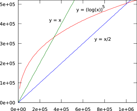
Figure 2: The recursion from $\psi$.

We will now sketch some ideas of how the $\psi$ statistic might “work.” An interesting feature of this statistic is that it converges on sequences of trees of increasing size satisfying certain conditions. For example, its value on an infinite balanced tree is approximately $5.05\times 10^{5}$, and on an infinite “comb” (perfectly imbalanced) tree its value is approximately $3.32\times 10^{5}$. The reasons for this are clear from Figure 2. The statistic can be evaluated on a large balanced tree by recursively iterating the function $x\mapsto\left(\log(2x)\right)^{5}$; from the plot it is clear that this recursion will converge to a value slightly more than $5\times 10^{5}$. For the comb tree the recursion is $x\mapsto\left(\log(x+8)\right)^{5}$, and the convergence value can again be estimated from the plot.

However, as can be seen from Table I, the convergence is not immediate. Furthermore, for small trees the statistic increases with imbalance (compare the balanced tree of depth three to the comb of depth seven, each of which have eight leaves), whereas on large trees the statistic increases with balance. This implies that the exchange of a comb subtree for a balanced subtree in a small tree can increase the statistic, whereas the same exchange in a large tree may decrease the statistic. This feature suggests that the TreeBASE trees may deviate from the “Markov branching” property of the beta-splitting models, which is that the distribution on subtrees of a given size is independent of the rest of the tree.

TABLE I: Calculation of the $\psi$ statistic

depth		balanced	comb
0		8	8
1		164	94.7
2		6.52e+03	2.04e+03
3		7.64e+04	2.58e+04
4		2.42e+05	1.08e+05
5		3.85e+05	2.09e+05
6		4.57e+05	2.76e+05
7		4.87e+05	3.09e+05

At this point it is important to emphasize that the $\psi$ statistic was invented for the single purpose of distinguishing the beta-splitting trees from the sorts of trees one finds in TreeBASE. This statistic was named for convenience only, not to introduce it into the canon of tree shape statistics. Indeed, one intent of this paper is to reduce the traditional emphasis on individual “general purpose” tree shape statistics and to focus instead on creating statistics for a specific application.

There will often be many such useful statistics. For example, note that a number of statistics appeared on different runs of the same objective function with similar performance. Because the space of algebraic expressions is so large and the fitness landscape is very “peaked,” runs of the genetic algorithm seldom converge on the same BRTSS when started with a different random seed or slightly different parameters.

The results of this section should not be construed as a rejection of the results or methodology of Blum and François. They found a value for $\beta$ which does in fact generate the observed level of overall balance for the TreeBASE trees. However, the above statistic shows that in this case there is more to tree shape than just overall balance. The difference between the two perspectives indicates interesting future directions for research. For example, is the observed difference due to reconstruction bias, or is the deviation indicated by the above statistic an actual feature of macroevolutionary processes? If the latter, how can we modify the present models to accommodate the difference?

IV Conclusions

In conclusion, we have developed a framework which allows enumeration of and optimization over a class of tree shape statistics. This class includes many of the tree shape statistics found in the literature. A genetic algorithm can be applied in this framework to find customized tree shape statistics for a certain application. The methodology is applied in an example case, finding a statistic which indicates a significant difference between two distributions on trees which was not previously evident.

Along with this new tool comes a new problem, which is that an automated system such as the genetic algorithm described above can create very complex tree shape statistics whose values can be hard to interpret. This issue is not problematic from an abstract statistical viewpoint, however it is comforting to have an intuitive interpretation of the statistics. In the sample case above some intuition was developed about a relatively simple statistic, but it may not be easy to find an interpretation for a complex one. It would be helpful in this regard to be able to derive limiting distributions for BRTSS applied to a distribution on trees. It is possible to do this for certain statistics, such as the number of cherries [7] or $I_{c}$ and $\bar{N}$ [9]. The methods used in the latter paper are applicable to a subclass of the BRTSS, however a substantial amount of work must be done on a case-by-case basis.

We note that the problem of differentiating two distributions on combinatorial objects has been approached in a different fashion by the statistical physics community. In their case, many models have been proposed for the growth of social and biological networks and a goal is to confirm or reject a certain model given some data. Analogous to the classical tree shape statistics, individual means of comparing graphs, such as the diameter or the number of subgraphs of a specific type, have been described (see, e.g. [18]). A more recent approach is to count in some manner the number of many different walks on the networks and then feed that information into a Support Vector Machine [19] [20]. This approach is similar to that described in the present paper in that machine learning is used to come up with tests which can distinguish models from data, however the actual technique is quite different. Their network approach focuses on local structure, while the BRTSS in this paper often provide global information. Nevertheless, an application of the network approach might provide some insights in the tree shape setting.

In the future we hope to use the methodology presented in this paper to expand the applications of tree shape theory in useful directions. For example, moderately sophisticated models of influenza evolution are currently being used to elucidate the evolutionary processes which form the remarkable imbalance of influenza phylogenetic trees [21] [22]. At this point very little of even the classical tree shape statistics are being applied for quantitative description. Another potentially underdeveloped area is the use of tree shape statistics to detect bias in modern tree reconstruction methods on real data; a lone article from over 10 years ago [23] forms the complete bibliography in this area.

References

- [1] M. Sackin, “Good and bad phenograms,” Syst. Zool., vol. 21, no. 2, pp. 225–226, 1972.
- [2] A. Mooers and S. Heard, “Evolutionary process from phylogenetic tree shape,” Q. Rev. Biol., vol. 72, no. 1, pp. 31–54, 1997.
- [3] M. Kirkpatrick and M. Slatkin, “Searching for evolutionary patterns in the shape of a phylogenetic tree,” Evolution, vol. 47, no. 4, pp. 1171–1181, 1993.
- [4] P. Agapow and A. Purvis, “Power of eight tree shape statistics to detect nonrandom diversification: A comparison by simulation of two models of cladogenesis,” Syst. Biol., vol. 51, no. 6, pp. 866–872, 2002.
- [5] D. Colless, “Phylogenetics: the theory and practice of phylogenetic systematics,” Syst. Zool., vol. 31, no. 1, pp. 100–104, 1982.
- [6] F. Matsen, “A geometric approach to tree shape statistics,” Systematic Biology, vol. 55, no. 4, pp. 652–661, 2006.
- [7] A. McKenzie and M. Steel, “Distributions of cherries for two models of trees,” Math. Biosci., vol. 164, no. 1, pp. 81–92, 2000.
- [8] K. Shao and R. Sokal, “Tree balance,” Syst. Zool., vol. 39, no. 3, pp. 266–276, 1990.
- [9] M. G. B. Blum, O. François, and S. Janson, “The mean, variance and joint distribution of two statistics sensitive to phylogenetic tree balance.” Ann. Appl. Prob., in press.
- [10] D. Richardson, “Some undecidable problems involving elementary functions of a real variable,” J. Symbolic Logic, vol. 33, pp. 514–520, 1968.
- [11] J. Moses, “Algebraic simplification: A guide for the perplexed,” Comm. ACM, vol. 14, pp. 527–537, 1971.
- [12] J. R. Koza, Genetic programming : on the programming of computers by means of natural selection, ser. Complex Adaptive Systems. Cambridge, MA: MIT Press, 1992.
- [13] W. J. Ewens, Mathematical population genetics. I, 2nd ed., ser. Interdisciplinary Applied Mathematics. New York: Springer-Verlag, 2004, vol. 27.
- [14] E. Chailloux, P. Manoury, and B. Pagano, Développement d’applications avec Objective CAML. Sebastopol, CA: O’Reilly, 2000, English translation available at http://caml.inria.fr/pub/docs /oreilly-book/.
- [15] M. G. B. Blum and O. François, “Which random processes describe the tree of life? a large-scale study of phylogenetic tree imbalance,” Syst. Biol., in press.
- [16] D. Aldous, “Stochastic models and descriptive statistics for phylogenetic trees, from Yule to today,” Stat. Sci., vol. 16, no. 1, pp. 23–34, 2001.
- [17] M. J. Sanderson, M. J. Donoghue, W. Piel, and T. Eriksson, “Treebase: a prototype database of phylogenetic analyses and an interactive tool for browsing the phylogeny of life.” Am. J. Bot., vol. 81, pp. 183–189, 1994.
- [18] B. Bollobás, Random graphs, 2nd ed., ser. Cambridge Studies in Advanced Mathematics. Cambridge: Cambridge University Press, 2001, vol. 73.
- [19] M. Middendorf, E. Ziv, C. Adams, J. Hom, R. Koytcheff, C. Levovitz, G. Woods, L. Chen, and C. Wiggins, “Discriminative topological features reveal biological network mechanisms,” BMC Bioinformatics, vol. 5, p. 181, Nov 2004.
- [20] M. Middendorf, E. Ziv, and C. H. Wiggins, “Inferring network mechanisms: the Drosophila melanogaster protein interaction network,” Proc Natl Acad Sci U S A, vol. 102, no. 9, pp. 3192–3197, Mar 2005.
- [21] V. Andreasen and A. Sasaki, “Shaping the phylogenetic tree of influenza by cross-immunity,” Theo. Pop. Biol., Apr 2006.
- [22] N. M. Ferguson, A. P. Galvani, and R. M. Bush, “Ecological and immunological determinants of influenza evolution,” Nature, vol. 422, no. 6930, pp. 428–433, Mar 2003.
- [23] D. H. Colless, “Relative symmetry of cladograms and phenograms: An experimental study,” Systematic Biology, vol. 44, no. 1, pp. 102–108, 1995.