Formation of regular spatial patterns in ratio-dependent predator-prey model driven by spatial colored-noise

Abstract

Results are reported concerning the formation of spatial patterns in the two-species ratio-dependent predator-prey model driven by spatial colored-noise. The results show that there is a critical value with respect to the intensity of spatial noise for this system when the parameters are in the Turing space, above which the regular spatial patterns appear in two dimensions, but under which there are not regular spatial patterns produced. In particular, we investigate in two-dimensional space the formation of regular spatial patterns with the spatial noise added in the side and the center of the simulation domain, respectively.

I Introduction

The influence of noise on nonlinear systems is the subject of intense experimental and theoretical investigations. The most well-known phenomenon is noise induces transition Horsthemke and Lefever (1984) and stochastic resonance Wiesenfeld and Moss (1995); Zhonghuai et al. (1998), both showing the possibility to transform noise into order.

In this paper, the problem of the predator-prey dynamical system Jost et al. (1999); Feedman and Mathsen (1993); Kuang and Beratta (1998); Bandyopadhyay and Chattopadhyay (2005); Mankin et al. (2006) is revisited and the results are presented concerning the noise aspects of the formation of spatial patterns in two dimensions. To our knowledge, the predator-prey dynamics in the absence of noise have been studied extensively using mathematical models. A common feature of these models is the prediction that the populations can cycle for some parameter sets: i.e. the populations of predators and prey do not settle to constant values, but rather, oscillate periodically in time. There are considerable data from field studies and laboratory experiments to support the existence of such population cycles. If a small group of predators are introduced into an spatial uniform population of prey, the predators will tend to invade the prey, leaving behind a mixture of predators and prey. In Jonathan A. Sherratt, Mark Lewis, Barry Eagan and Andrew Fowler’s works Sherratt et al. (1997, 1995), they have studied the behavior of such invasions for cyclic populations. The results are somewhat surprising: the invasion leaves behind spatiotemporal oscillations falling into either periodic traveling waves or spatiotemporal irregularity; mixed behavior also occurs.

One of the key issues in ecology is how environmental fluctuation and species interaction determine variability of the population density McGlade (1999); Levin et al. (1997); Ripa and Ives (2003). The other topic is that dynamic patterns in two-dimensional space have recently been introduced into ecology Sayama et al. (2002, 2000); Zillio et al. (2005); Dieckmann et al. (2000). Ecologists have mainly been interested in the dynamical consequences of population interactions, often ignoring environmental variability altogether in space. However, the essential role of environmental fluctuations has recently been recognized in theoretical ecology. Noise-induced effects on population dynamics have been subject to intense theoretical investigations Vilar and Solé (1998); Abramson and Zanette (1998); McKane et al. (2000); Mankin et al. (2002, 2004); Sauga and Mankin (2005); Mankin et al. (2006); Houchmandzadeh (2002); Chesson (2003); Kinezaki et al. (2003). Moreover, ecological investigations suggest that population dynamics is sensitive to noise. In spite of the obvious significance of this circumstance, the role of non-equilibrium spatial fluctuations (spatial noise) of environmental has not been investigated much in the context of ecosystems.

Recently, the general N-species Lotka-Volterra and ratio-dependent predator-prey dynamical systems are described as stochastic models by Romi Mankin, Ako Sauga and et al. i.e. add the parameter noise term in the classical models, where the carrying capacity of the population is taken into account as dichotomous noise. For former model, the result of the study has shown that the noise induces discontinuous transitions from a stable state to an instable one in Refs. Mankin et al. (2002, 2004). The latter model Mankin et al. (2006) has shown that the phenomena of colored-noise-induced Hopf bifurcation and corresponding reentrant transitions can appear in ecosystems. But both models are studied in nonspatial. From the Refs. Sherratt et al. (1997); Alonso et al. (2002); Pascual (1993) we know that the space plays a crucial role in the ecosystem. In Ref. Pascual (1993), the results have shown that the Turing patterns occur in the ratio-dependent predator-prey models. Thus, naturally arise a problem that how the spatial noise influences the formation of spatial patterns or species invasion in the ratio-dependent predator prey dynamical systems? Here we address how the spatial noise affects the formation of the spatial patterns on the coexistence equilibrium in the reaction-diffusion predator-prey dynamical systems.

II Model

II.1 The ratio-dependent model with diffusion

We consider the reaction-diffusion model for predator-prey interactions. At any point $(x,y)$ at time $T$, the dynamics of prey ($N(x,y;T)$) and predator ($P(x,y;T)$) populations are given by a reaction-diffusion model with logistic growth of the prey and a type II (or Michaelis-Menten-type) function response of the predator

$$\frac{\partial N}{\partial T}=rN(1-\frac{N}{K})-\frac{bN}{kP+N}P+D_{1}\nabla^{2}N,$$ (1a)

$$\frac{\partial P}{\partial T}=e\frac{bN}{kP+N}P-\mu P+D_{2}\nabla^{2}P,$$ (1b)

where $\nabla^{2}$ is the Laplacian operator in Cartesian coordinates. The parameters $r$, $K$, $\mu$ and $e$ denote the intrinsic growth rate, carrying capacity of the prey, the death rate of the predator and the yield coefficient of prey to predator, respectively. The constant $D_{1}$ and $D_{2}$ are prey and predator diffusion coefficients, respectively.

The model (1) can be simplified by introducing the dimensionless variables, $n=N/K$, $p=Pk/K$, $t=Tr$, $x=x/\sqrt{D_{1}/r}$, and $y=y/\sqrt{D_{1}/r}$. The units of the dimensional variables will be scaled. Thus, in the terms of these dimensionless variables the model is simplified to

$$\frac{\partial n}{\partial t}=(1-n)n-\frac{\beta np}{n+p}+\nabla^{2}n,$$ (2a)

$$\frac{\partial p}{\partial t}=\varepsilon\beta\frac{np}{n+p}-\eta p+d\nabla^{2}p,$$ (2b)

where four new dimensionless parameters naturally arise:

$$\beta=\frac{b}{kr},\eta=\frac{\mu}{r},\varepsilon=ek,d=\frac{D_{1}}{D_{2}}.$$ (3)

From the Ref. Jost et al. (1999), we know that the ratio-dependent predator-prey dynamical system (2) has a homogeneous coexistence point, $(n_{s},p_{s})$, i.e. the coexistence point is given by

$$n_{s}=1-(\eta/\varepsilon)(\Delta),p_{s}=(\Delta-1)n_{s},$$ (4)

where $\Delta=\varepsilon\beta/\eta$. This coexistence point is biologically meaningful ($n_{s}>0,p_{s}>0$) only if $\eta>\varepsilon(\beta-1)$ and $\eta<\varepsilon\beta$

Since we focus on the spatial noise affects the formation of the spatial patterns in the ratio-dependent predator-prey system, we don’t show the mathematical property here.

II.2 Spatial noise in predator-prey model

Environmental fluctuations and other factors (see the discussion) are important components in an ecosystem. In Refs. May (1972, 2001), May have pointed out the fact that because of environmental fluctuations, the carrying capacities, death rates, birth rates, and other parameters involved with the systems exhibit random fluctuations to a greater or lesser extent. Because a multinoise fluctuation stochastic system is difficult to consider analytically, it is generally reasonable to confine only one (or two) parameter of the system to fluctuate. In our paper, a random interaction with the environment (such as climate, disease, etc) in some domain is taken into account by introducing a random spatial noise ($\xi(x,y;t)$) to the prey. Henceforth, the dynamic system (2) is used to numerical simulation. In comparison with Refs. Mankin et al. (2002, 2004); Sauga and Mankin (2005); Mankin et al. (2006), here the difference is that we take into account the spatial noise in two dimensions. For the spatial noise we choose the colored noise $\xi(x,y;t)$, which accounts for density fluctuations at point $(x,y)$. The Ornstein-Uhlenbeck process was used to calculate the colored-noise (Appendix). To characterize the spatial noise, we introduce parameter, $D$, the intensity of the noise. The $\xi(x,y;t)$ has the following properties:

$$\langle\xi(x,y;t)\rangle=0$$

and

$$\langle\xi(x,y;t)\xi(x^{\prime},y^{\prime};t^{\prime})\rangle=D^{2}\delta(x-x^{\prime})\delta(y-y^{\prime})e^{-|t-t^{\prime}|/\tau}.$$

Obviously, $\tau$ is the noise correlation time. Although the dynamical system (2) absent of random spatial noise term is well understood, there is little analytic theory for the system in two-dimensional space. The equations are integrated numerically with an implicit scheme using $200\times 200$ an $50\times 200$ spatial grid sites, respectively. For nonlinear equations, the discretization introduced by numerical methods may generate spurious results. To test this possibility, the resolution of the simulation result was increased with space and time, and the system is integrated with a different scheme, a finite difference method. In all case the same qualitative results have been obtained. We assume zero flux boundary conditions for all $t$ in the simulation.

III Results

We study the effect of the spatial noise to the formation of the spatial patterns. The results presented here are based on numerical analysis for a set of parameters, $\beta=2$, $\varepsilon=0.5$, $\eta=0.6$, $d=10$ MIS , $\Delta h=0.5$ (space scales), and $\Delta t=0.005$ (time step), chosen to obtain large-scale spatial patterns in the absence of spatial noise (see Fig. 1). Moreover, from Turing Structures theory we know that these parameters must be within the Turing space. In fact, the authors Alonso et al. (2002) have validated that these parameters are in the Turing space.

Figure 1 illustrates the irregular spatial patterns behavior of prey numbers in two dimensions absent of the spatial noise. From this figure one can see that the spatial patterns are irregular in two dimensions when they reach the steady state.

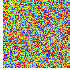
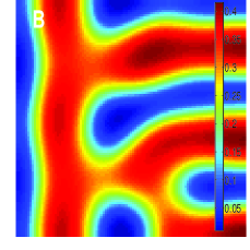
Figure 1: (Color online) Spatial patterns in two dimensions absent of noise (in this case, the qualitative results are the same as the Ref. Alonso et al. (2002)). The numerical integration of the dynamical system described by Eqs. (2) has been performed in a $200\times 200$ lattices. (A) $t=0$ and (B) $t=550$. The right inset shows the color corresponding to the value of prey.

The main results in our paper show the effect of spatial noise with respect to formation of the spatial patterns. In order to ensure the facticity of the result, we have studied the system (2) in two cases driven by the spatial noise. First, we introduce the spatial noise (here the spatial noise is perturbation on the equilibrium value) at the left of the $50\times 100$ spatial grid sites. The domain of the spatial noise is set by $50\times 3$. The ecological significance of the spatial noise can be explained for the invasion of a prey population by predators in the space (see Fig. 2(A)). Second, we introduce the spatial noise (here the spatial noise is the same as that in first) at the center of the $200\times 200$ spatial grid sites (see Fig. 2(B)).

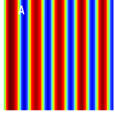
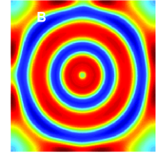
Figure 2: (Color online) Spatial patterns in two dimensions driven by spatial noise. The numerical integration of the dynamical system described by Eqs. (2) has been performed in $50\times 200$ and $200\times 200$ lattices, respectively. (A) The spatial noise is added at the left-hand side of the $50\times 200$ lattice; (B) The spatial noise is added at the center of the $200\times 200$ lattices.

Figure 2 illustrates the formation of the regular spatial patterns behavior of the prey numbers in two dimensions after the spatial patterns reach the steady state, where the initially condition (at $t=0$) add random and nonuniform small perturbations to the equilibrium values. The maximum amplitude of the perturbations is less than $0.0005$ and the noise correlation time $\tau=1$. The intensity of the spatial noise is equal to 0.05. Comparing Fig. 1 with Fig. 2, one can easily find that some characteristics are the same (here mainly relate to the wavelength). But Fig. 2(A) and Fig. 2(B) both appear periodical structure patterns in two dimensions (called the spatial-period-2-structure). Additionally, these spatial patterns are regular in two dimensions. The only difference is that In Fig. 2(A) the spatial patterns are stripe but in Fig. 2(B) target when the system reach steady state.

If we change the direction of observing angle, the space vs density plot can be seen more clearly. The space plot of the variable $n$ is shown in Fig. 3, where the horizontal axis represents the horizontal spatial line crossing the center point. Fig. 3 corresponds to Fig. 2(B).

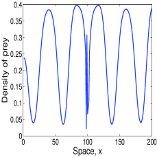
Figure 3: This graph illustrates the regular patterns driven by the spatial noise from other views.

Finally, we increase the intensity of the spatial noise in the system, and the results show that for every initial condition there is a critical value of the intensity of noise, $D_{\rm c}$. Here the critical value $D_{\rm c}\approx 0.02$ with foregoing parameter. Above the critical value the regular spatial patterns appear and maintain in two dimensions. However, under the critical value, there doesn’t exist regular spatial patterns even though the simulation runs a long time. The qualitative results are the same under different $D$ values (above the critical value), so we only show typical results as in Fig. 2 when $D=0.05$. Under the critical value, the result is not shown in our paper since the spatial patterns are similar to Fig. 1.

IV Conclusion and discussion

In our paper we have considered the effect of the spatial noise with respect to the spatial patterns in the ratio-dependent predator-prey system in two dimensions. The results show that there exits a critical value of the intensity of the spatial noise ($D_{\rm c}$) for the system (2) when the parameters are in the Turing space. Above the critical value the regular spatial patterns appear in two-dimensional space, but under the critical value there doesn’t exit regular spatial patterns. Our key objective is that the regular spatial patterns can appear in ratio-dependent predator-prey model driven by spatial noise. Here, we use the intensity of the noise to characterize the spatial noise, one can also use other measures to characterize the spatial noise (e.g signal to noise ratio).

Our results differ in several ways from the previous studies of predator-prey equations in ecology Murray (1989); McKane et al. (2000); Mankin et al. (2002, 2004); Sauga and Mankin (2005); Mankin et al. (2006). Previous studies have shown that the diffusion can induce instability and the parameter noise can induce Hopf-bifurcation, discontinuous transition and so on. But here we investigate the spatial noise in the system (2) in two dimensions. Our results suggest a direction for further research, which is how to detect the spatial fluctuation of the complex dynamics in natural environments. In addition, two species predator-prey systems exhibit Turing spatial patterns only under special conditions. In Ref. Alonso et al. (2002), the study suggests that any strategy that involves interference between predators should enhance patterns formation. Furthermore, the process rates (prey birth rate, predator death rate, predator attack rate) and the mobility of population size can also be determining factors in the formation of biological patterns.

Appendix

The colored noise satisfies

$$\langle\xi(t)\rangle = 0,$$ (5)

$$\langle\xi(t)\xi(t^{\prime})\rangle = D^{2}e^{-|t-t^{\prime}|/\tau}.$$

It can be shown that the colored noise $\xi(t)$ my be calculated form the following equation

$$\frac{d\xi}{dt} = -\frac{1}{\tau}+\frac{D\sqrt{2\tau}}{\tau}\eta(t),$$ (6)

where $\eta(t)$ is a Gaussian white noise source with

$$\langle\eta(t)\rangle = 0,$$

$$\langle\eta(t)\eta(t^{\prime})\rangle = \delta(t-t^{\prime}).$$

Equation (6) describes an Ornstein-Uhlenbeck process Higham (2001), and it can be shown that the solution to this equation satisfies Eqs. (5).

V Acknowledgments

This work was supported by the National Natural Science Foundation of China under Grant No. 10471040 and the Science Foundation of Shan’xi Province Grant No. 2006011009.

References

- Horsthemke and Lefever (1984) W. Horsthemke and R. Lefever, Noise-induce transitions (Springer-Verlag, Berlin, 1984).
- Wiesenfeld and Moss (1995) K. Wiesenfeld and F. Moss, Nature 373, 33 (1995).
- Zhonghuai et al. (1998) H. Zhonghuai, Y. Lingfa, X. Zuo, and X. Houwen, Phys. Rev. Lett. 81, 2854 (1998).
- Jost et al. (1999) C. Jost, O. Arino, and R. Arditi, Bull. Math. Biol. 61, 19 (1999).
- Feedman and Mathsen (1993) H. I. Feedman and R. M. Mathsen, Bull. Math. Biol. 55, 817 (1993).
- Kuang and Beratta (1998) Y. Kuang and E. Beratta, J. Math. Biol. 36, 389 (1998).
- Bandyopadhyay and Chattopadhyay (2005) M. Bandyopadhyay and J. Chattopadhyay, Nonlinearity 18, 913 (2005).
- Mankin et al. (2006) R. Mankin, T. Laas, A. Sauga, and A. Ainsaar, Phys. Rev. E 74, 021101 (2006).
- Sherratt et al. (1997) J. A. Sherratt, B. T. Eagan, and M. A. Lewis, Phil. Trans. R. Soc. B 352, 21 (1997).
- Sherratt et al. (1995) J. A. Sherratt, M. A. Lewis, and A. C. Fowler, Proc. Natl. Acad. Sci. USA 92, 2524 (1995).
- McGlade (1999) J. McGlade, Advanced Ecological Theory: Principles and Applications (Blackwell Science, London, 1999).
- Levin et al. (1997) S. A. Levin, B. Grenfell, A. Hastings, and A. S. Perelson, Science 275, 334 (1997).
- Ripa and Ives (2003) J. Ripa and A. R. Ives, Theor. Popul. Biol. 64, 369 (2003).
- Sayama et al. (2002) H. Sayama, M. A. M. d. Aguiar, Y. Bar-Yam, and M. Baranger, Phys. Rev. E 65, 051919 (2002).
- Sayama et al. (2000) H. Sayama, L. Kaufman, and Y. Bar-Yam, Phys. Rev. E 62, 7065 (2000).
- Zillio et al. (2005) T. Zillio, I. Volkov, J. R. Banavar, S. P. Hubbell, and A. Maritan, Phys. Rev. Lett. 95, 098101 (2005).
- Dieckmann et al. (2000) U. Dieckmann, R. Law, and J. A. J. Metz, The Geometry of Ecological interactions: Simplifying spatial complexity (Cambridge University Press, U K, 2000).
- Vilar and Solé (1998) J. M. G. Vilar and R. V. Solé, Phys. Rev. Lett. 80, 4099 (1998).
- Abramson and Zanette (1998) G. Abramson and D. H. Zanette, Phys. Rev. E 57, 4572 (1998).
- McKane et al. (2000) A. McKane, D. Alonso, and R. V. Solé, Phys. Rev. E 62, 8466 (2000).
- Mankin et al. (2002) R. Mankin, A. Ainsaar, A. Haljas, and E. Reiter, Phys. Rev. E 65, 051108 (2002).
- Mankin et al. (2004) R. Mankin, A. Sauga, A. Ainsaar, A. Haljas, and K. Paunel, Phys. Rev. E 69, 061106 (2004).
- Sauga and Mankin (2005) A. Sauga and R. Mankin, Phys. Rev. E 71, 062103 (2005).
- Houchmandzadeh (2002) B. Houchmandzadeh, Phys. Rev. E 66, 052902 (2002).
- Chesson (2003) P. Chesson, Theor. Popul. Biol. 64, 345 (2003).
- Kinezaki et al. (2003) N. Kinezaki, K. Kawasaki, F. Takasu, and N. Shigesada, Theor. Popul. Biol. 64, 291 (2003).
- Alonso et al. (2002) D. Alonso, F. Bartumeus, and J. Catalan, Ecology 83, 28 (2002).
- Pascual (1993) M. Pascual, Proc. R. Soc. Lond. B 251, 1 (1993).
- May (1972) R. M. May, Science 177, 900 (1972).
- May (2001) R. M. May, stability and complexity in model ecosytems (Princeton University Press, Princeton, 2001).
- (31) Note, Since predator must diffuse faster than prey in order to have the spatial patterns appearance, . A. Okubo, Diffusion and ecological problems: mathematical models (Springer-Verlag, Berling, Germany, 1980).
- Murray (1989) J. D. Murray, Mathematical Biology (Springer-Verlag, New York, 1989).
- Higham (2001) D. J. Higham, SIAM Review 43, 525 (2001).