Radiation Pressure Induced Einstein-Podolsky-Rosen Paradox

Abstract

We demonstrate the appearance of Einstein-Podolsky-Rosen (EPR) paradox when a radiation field impinges on a movable mirror. Then, the possibility of a local realism test within a pendular Fabry-Perot cavity is shown to be feasible.

Quantum Optics is widely used to perform fundamental tests of Quantum Mechanics. Essentially, the reason relies on the fact that the only relevant noise at optical frequency is the vacuum noise, and on the possibility of generating non-classical states through nonlinear media. Recently, however, much of theoretical attention has also been devoted to opto-mechanical systems [1]. On the other hand, due to technological developments, those systems are now becoming experimentally accessible [2].

Along this line, we would deal with the interesting question of whether radiation pressure can induce entanglement. Entanglement is, indeed, the source of many mysteries of Quantum Mechanics and it is the fundamental concept involved in what is called the spooky action-at-a-distance [3]. In this respect our analysis will show that entanglement can be obtained via a macroscopic object. It is not quite entanglement between macroscopic objects but it will be shown that it is mediated by a macroscopic body. To this end we consider the radiation field impinging on a movable mirror and we will study the properties of the reflected field. The quantum noise reduction for such a model has been predicted [4], however, we demonstrate here that the state of the radiation field interacting with a macroscopic object can become non-classical at a level deeper than simple squeezing. Namely, we demonstrate the appearance of EPR aspects [3] on continuous variables in that system.

Our analysis starts from the EPR paradox theoretically formulated in Refs. [5, 6], where the roles of canonical position and momentum variables, of the original EPR paper [3], are played by the amplitude and phase quadratures of the output signals belonging to two distinct cavity modes. In this scheme the quadratures $\{\hat{X}_{1},\hat{Y}_{1}\}$ of the first mode are inferred in turn from measurements of the quadratures $\{\hat{X}_{2},\hat{Y}_{2}\}$ of the second mode, which is let spatially separate from the first. The errors of these inferences are then quantified by the variances

$$\Delta_{\rm inf}^{2}\hat{X}(g_{X})\equiv\left\langle\left(\hat{X}_{1}-g_{X}\hat{X}_{2}\right)^{2}\right\rangle\hskip 36.135pt\Delta_{\rm inf}^{2}\hat{Y}(g_{Y})\equiv\left\langle\left(\hat{Y}_{1}-g_{Y}\hat{Y}_{2}\right)^{2}\right\rangle$$ (1)

where $g_{X}$ and $g_{Y}$ are two dimensionless scaling factors, which we will adjust to allow for the greatest accuracy in inferred determinations of $\{\hat{X}_{1},\hat{Y}_{1}\}$. As pointed out in Ref. [6], an experimental demonstration of the EPR paradox occurs when the product of the errors of the inferences will be less than the limit imposed by the Heisenberg principle for the observables $\{\hat{X}_{1},\hat{Y}_{1}\}$. Of course, in order to obtain such a result the modes have to be strongly correlated. In the original proposal of Refs. [5, 6] and in the experimental realization of Ref. [7], the necessary correlation was obtained by a nondegenerate optical parametric oscillator, which makes interact the two modes inside the cavity.

Here, instead, they indirectly interact, by means of the radiation pressure by which each of them acts on one of the cavity mirrors, which is let free to oscillate and assumed perfectly reflecting. The other mirror is instead assumed fixed and with non zero transmittivity. When the cavity is empty the moving mirror undergoes harmonic oscillations damped by the coupling to an external bath in equilibrium at temperature $T$. As pointed out in Ref. [8], under the assumption that the measurement time is of the order of the mechanical relaxation time of the mirror, it is possible to consider such a macroscopic oscillator as a quantum oscillator. The cavity resonances are calculated in the absence of the impinging field, hence if $L$ is the equilibrium cavity length the resonant frequency of the cavity will be $\omega_{c}=nc/2L$, where $n$ is an arbitrary integer number and $c$ the speed of light. Furthermore, we assume that at the frequency of the impinging field $\omega_{0}$, the fixed mirror does not introduce any excess noise beyond the input field noise. We also assume that retardation effects, due to the oscillating mirror in the intracavity field, are negligible. We shall use a field intensity such that the correction to the radiation pressure force, due to the Doppler frequency shift of the photons [9] on the moving mirror, is completely negligible. This means considering the damping coefficient of the oscillating mirror to be only due to the coupling with the thermal bath. Thus, the Hamiltonian for this system can be written as

$${\hat{H}}=\hbar\omega_{c}\left({\hat{A}}_{1}^{\dagger}{\hat{A}}_{1}+{\hat{A}}_{2}^{\dagger}{\hat{A}}_{2}+1\right)+\frac{\hat{P}^{2}}{2m}+\frac{1}{2}m\,\omega_{m}\hat{Q}^{2}+{\hat{H}}_{int}$$ (2)

where ${\hat{A}}_{1}$ and ${\hat{A}}_{2}$ are the annihilation operators of the two cavity modes, which are supposed to have the same frequency and mutually orthogonal polarizations; $\hat{P}$ and $\hat{Q}$ are the momentum and the displacement operators, respectively, from the equilibrium position of the oscillating mirror with mass $m$ and oscillation frequency $\omega_{m}$. The mechanical frequency $\omega_{m}$ will be many orders of magnitude smaller than $\omega_{c}$ to ensure that the number of photons generated by the Casimir effect is completely negligible [10]. ${\hat{H}}_{int}$ accounts for the interaction between the cavity modes and the oscillating mirror [11]. Since we have assumed no retardation effects, ${\hat{H}}_{int}$ simply represents the effect of the radiation pressure force which causes the instantaneous displacement $\hat{Q}$ of the mirror [4, 12]:

$${\hat{H}}_{int}=-\hbar\omega_{c}\,\left({\hat{A}}_{1}^{\dagger}{\hat{A}}_{1}+{\hat{A}}_{2}^{\dagger}{\hat{A}}_{2}\right)\;\hat{Q}/L\;.$$ (3)

Now, we assume that the intracavity radiation fields are damped through the output fixed mirror at the same rate $\gamma_{c}$, while $\gamma_{m}$ is the mechanical damping rate for the mirror’s Brownian motion. The interaction (3) gives rise to nonlinear Langevin equations whose linearization around the steady state leads to

$$\left\{\begin{array}[]{l}\frac{d}{dt}\,\hat{q}(t)=\frac{1}{m}\hat{p}(t)\,,\\ \\ \frac{d}{dt}\,\hat{p}(t)=-m\,\omega_{m}^{2}\hat{q}(t)-2\,\gamma_{m}\hat{p}(t)+\hbar\omega_{c}\frac{|\alpha_{1}|}{L}\left({\hat{a}}_{1}(t)+{\hat{a}}_{1}^{\dagger}(t)\right)+\hbar\omega_{c}\frac{|\alpha_{2}|}{L}\left({\hat{a}}_{2}(t)+{\hat{a}}_{2}^{\dagger}(t)\right)-{\hat{\xi}}(t)\,,\\ \\ \frac{d}{dt}\,{\hat{a}}_{j}(t)=\left(i\Delta-\frac{1}{2}\right)\gamma_{c}{\hat{a}}_{j}(t)+i\omega_{c}\frac{|\alpha_{j}|}{L}\hat{q}(t)+{\hat{a}}_{j}^{\rm in}(t)\,,\hskip 36.135pt\hskip 7.22743ptj=1,2\end{array}\right.$$ (4)

where now all the operators represent small fluctuations around steady state values, i.e. $\hat{Q}(t)=x+\hat{q}(t)$, $\hat{P}(t)=y+\hat{p}(t)$, ${\hat{A}}_{j}(t)=\big{(}\alpha_{j}+{\hat{a}}(t)\big{)}\exp[-i(\omega_{0}t-\arg{\alpha_{j}})]$. The steady state is determined by

$$\begin{array}[]{llll}x\equiv\langle{\hat{Q}}\rangle_{ss}=\frac{\hbar\omega_{c}}{m\omega_{m}^{2}L}\left(|\alpha_{1}|^{2}+|\alpha_{2}|^{2}\right)\,,&&&y\equiv\langle{\hat{P}}\rangle_{ss}=0\,,\\ \\ \alpha_{j}\equiv\langle{\hat{A}}_{j}\rangle_{ss}e^{i\omega_{0}t}=\frac{\sqrt{\gamma_{c}}\alpha_{j}^{in}}{(1/2-i\Delta)\gamma_{c}}\,,&&&\Delta=(\omega_{0}-\omega_{c}+\omega_{c}x/L)/\gamma_{c}\,,\\ \end{array}$$ (5)

where $\alpha_{j}^{in}$ is the classical field characterizing the input laser power $P_{in}=\hbar\omega_{0}\left(|\alpha_{1}^{in}|^{2}+|\alpha_{2}^{in}|^{2}\right)$. In the following we assume that the laser pumps both the cavity modes in the same way, i.e. $\alpha_{1}^{in}=\alpha_{2}^{in}$: this allows for identical coupling constants between the two modes and the mirror, $\alpha_{1}=\alpha_{2}=\alpha$. Moreover, $\Delta$ is the (dimensionless) radiation phase shift due to the detuning and to the stationary displacement of the mirror. ${\hat{a}}^{\rm in}_{j}(t)$ is the vacuum noise operator at the input of the $j$-th cavity mode. Instead, ${\hat{\xi}}(t)$ is the noise operator for the quantum Brownian motion [13] of the mirror. The non vanishing noise correlations are

$$\langle{\hat{a}}^{\rm in}_{j}(t)[{\hat{a}}^{\rm in}_{k}]^{{\dagger}}(t^{\prime})\rangle = \gamma_{c}\delta(t-t^{\prime})\,\delta_{j,k}\,,\quad j,k=1,2\,,$$ (6)

$$\langle{\hat{\xi}}(t){\hat{\xi}}(t^{\prime})\rangle = \frac{m\gamma_{m}}{\pi}\int\,d\omega\,\left\{\hbar\omega\left[\coth\left(\frac{\hbar\omega}{2k_{B}T}\right)-1\right]\right\}e^{i\omega(t-t^{\prime})}\,,$$ (7)

where $k_{B}$ is the Boltzmann constant and $T$ the equilibrium temperature.

The boundary relation for the radiation fields is [14]

$${\hat{a}}^{\rm out}_{j}(t)=\gamma_{c}\,{\hat{a}}_{j}(t)-{\hat{a}}^{\rm in}_{j}(t)\,.$$ (8)

From Eq. (4) we can see that the cavity modes ${\hat{a}}_{1}(t)$ and ${\hat{a}}_{2}(t)$, mutually interact by means of the action of the mirror displacement operator. In particular this coupling is linear and it seems to be able to create correlation between the modes quadratures, which in turn can be revealed in the output field. At the beginning of this letter we have adopted an heuristic approach in order to introduce the problem. We considered the quadrature operators of the signal modes as effective measurable quantities, which obey the canonical commutation rules that permit us to write down an Heisenberg’s relation by which testing the EPR paradox. However, in the case of a signal outgoing from a cavity one has to be careful, since the commutation rules at two distinct time is a Dirac delta function of the difference of the time values considered [14]: this means that it is impossible to write down an effective uncertainty relation for their quadratures. The solution for this problem is to consider such operators in the frequency domain instead of the time domain [5, 6].

Thus, given the quadrature

$$\hat{X}^{\rm out}_{j}(\phi,t)={\hat{a}}^{\rm out}_{j}(t)e^{-i\phi}+[{\hat{a}}^{\rm out}_{j}(t)]^{{\dagger}}(t)e^{i\phi}\,,$$ (9)

we define

$$\hat{{\widetilde{X}}}^{\rm out}_{j}(\phi,\omega)=\frac{1}{\sqrt{\tau}}\int_{-\tau/2}^{\tau/2}\,dt\,e^{i\omega t}\,\hat{X}^{\rm out}_{j}(\phi,t)\;,$$ (10)

where $\tau$ is the measurement time of the output signal. $\hat{\widetilde{X}}^{\rm out}_{j}(\phi,\omega)$ is a sort of Fourier transform of $\hat{X}^{\rm out}_{j}(\phi,t)$ on a limited time interval, which has some interesting properties. For example, in the limit of $\tau$ greater than the coherence time of the signal, the expectation values of the product of $\hat{\widetilde{X}}^{\rm out}_{j}(\phi,\omega)$ with $\hat{\widetilde{X}}^{\rm out}_{k}(\varphi,\omega)$ is the power density spectrum of the original quadrature fluctuations product, namely

$$S_{j,k}(\omega,\phi,\varphi)=\left\{\int dt^{\prime}e^{i\omega t^{\prime}}\langle\;\hat{X}^{\rm out}_{j}(\phi,t)\;\hat{X}^{\rm out}_{k}(\varphi,t^{\prime}-t)\rangle\right\}_{t}\;,$$ (11)

where $\{\cdots\}_{t}$ means averaging $t$ on the time interval $\tau$. $S_{j,k}(\omega,\phi,\varphi)$ is simply related to the spectral density photocurrent fluctuations, which is possible to measure by means of separated balanced homodyne detection of the two signal (see for example Ref. [7]). In the rest we focus on the case with $\omega=0$. Notice that this is the only case in which the operators (10) are Hermitian. Furthermore, the commutation relation between $\hat{\widetilde{X}}^{\rm out}_{j}(\phi,0)$ and $\hat{\widetilde{X}}^{\rm out}_{k}(\phi+\pi/2,0)$ is exactly equal to $2i\gamma_{c}\delta_{j,k}$ as it is possible to verify from the properties of the output signals. This means that $\{\hat{\widetilde{X}}^{\rm out}_{1}(0,0),\hat{\widetilde{X}}^{\rm out}_{1}(\pi/2,0)\}$ and $\{\hat{\widetilde{X}}^{\rm out}_{2}(0,0),\hat{\widetilde{X}}^{\rm out}_{2}(\pi/2,0)\}$ are two mutually independent couples of conjugate observables. The only constraint in order to use them in an EPR paradox realization, is to ensure that the measurements on the first mode are spatially separated from those of the second mode. In particular this means $c\tau/d<1$, with $d$ the spatial distance between the balanced homodyne receivers of the modes.

Now, by Fourier transforming Eqs. (4) it is possible to get the output field quadratures by means of Eq.(8) and then one can evaluate the inferences errors (1). Choosing of inferring $\hat{\widetilde{X}}^{\rm out}_{1}(0,0)$ and $\hat{\widetilde{X}}^{\rm out}_{1}(\pi/2,0)$ with $\hat{\widetilde{X}}^{\rm out}_{2}(0,0)$ and $\hat{\widetilde{X}}^{\rm out}_{2}(\pi/2,0)$ respectively, we obtain

$$\Delta^{2}_{\rm inf}\hat{\widetilde{X}}^{\rm out}_{1}(\phi,0)=\sum_{j,k=1}^{2}(-)^{j+k}\,g_{\phi}^{j+k-2}\,S_{j,k}(0,\phi,\phi)\,,$$ (12)

and minimizing the inference errors by the scaling factors $g_{\phi}$ introduced in Eq. (1), the above equation reduces to

$$\Delta_{\rm inf}^{2}\hat{\widetilde{X}}^{\rm out}_{1}(\phi,0)=\gamma_{c}\left(1+\frac{\epsilon(\phi)}{1+\epsilon(\phi)}\right)\,,$$ (13)

with

$$\epsilon(0)=\left(\frac{{\cal T}-1}{2}\right)\frac{\cal P}{\left({\Delta}^{2}+{\cal P}+1/4\right)^{2}}\;,\hskip 36.135pt\epsilon(\pi/2)=\left(\frac{{\Delta}^{2}+{\cal P}+{\cal T}/4}{2{\Delta}^{2}}\right)\frac{\cal P}{\left({\Delta}^{2}+{\cal P}+1/4\right)^{2}}\;,$$ (14)

where we have introduced the dimensionless power and temperature ${\cal P}=8\omega_{0}{\Delta}P_{in}/mL^{2}\omega_{m}^{2}\gamma_{c}^{2}(1+4\Delta^{2})$, ${\cal T}=8k_{B}T\gamma_{m}\Delta/\hbar\omega_{m}^{2}$. These become now the fundamental variables of our system.

The EPR paradox will be verified if the product of the inference errors $\Delta_{\rm inf}^{2}\hat{\widetilde{X}}^{\rm out}(0,0)$ and $\Delta_{\rm inf}^{2}\hat{\widetilde{X}}^{\rm out}(\pi/2,0)$ is less than the minimum uncertainty limit imposed by the commutation relation between $\hat{\widetilde{X}}^{\rm out}_{1}(0,0)$ and $\hat{\widetilde{X}}^{\rm out}_{1}(\pi/2,0)$; that means, with the aid of Eq. (13),

$$\left(1+\frac{\epsilon(0)}{1+\epsilon(0)}\right)\left(1+\frac{\epsilon(\pi/2)}{1+\epsilon(\pi/2)}\right)<1\;.$$ (15)

From Eq. (14) results that $\epsilon(\pi/2)$ is always positive; so, the term in the second brackets on the l.h.s. of Eq. (15) is always greater than $1$. Then, we can verify the EPR paradox if the term in the first brackets on the l.h.s. of Eq. (15) becomes smaller than 1. That depends on $\epsilon(0)$ which, for ${\cal T}<1$, can be a negative number.

In Fig.1 we show the l.h.s. of Eq.(15) as function of ${\cal P}$ and ${\cal T}$. We see how the thermal noise related to the Brownian motion of the mirror plays a detrimental role, in fact as soon as ${\cal T}$ increases, the region of possible values of ${\cal P}$ tends to become narrower and to disappear. Notice that writing back $P_{in}$ in terms of ${\cal P}$, the limit $\Delta\to 0$ cannot be performed; this is consistent with Eqs.(4) where in such a limit only the amplitude quadratures become correlated, hence no paradox can arise.

For grant, we take from the graph ${\cal P}=0.17$ and ${\cal T}=0.1$ which can be obtained with the following values of parameters: $m=3\times 10^{-5}$ Kg, $L=10^{-3}$ m, $\omega_{m}=2$ MHz, $\gamma_{m}=1$ Hz, $\omega_{c}\simeq\omega_{0}=2\times 10^{15}$ Hz, $\gamma_{c}=2$ MHz, $T\simeq 4\;^{\circ}{\mbox{K}}$ and $P_{in}\simeq 30\mbox{mW}$. These correspond to the experimental set up of Ref. [15], and give the value $0.7$ for the l.h.s. of Eq.(15). Of course, better results can be achieved by means of an optimization of all parameters or by working with microfabricated cantilever [16].

In conclusion, we have proposed a ponderomotive scheme to get entanglement of radiation fields. The resulting correlations give rise to EPR paradox and seem quite robust notwithstanding they derive from the action of a macroscopic object. Furthermore, the numerical results show that the proposed test can be realized with the present technology.

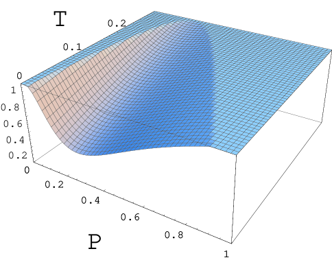
FIG. 1.: The l.h.s. of Eq.(15) is plotted vs. ${\cal P}$ and ${\cal T}$ for $\Delta=0.18$.

REFERENCES

- [1] See, e.g., S. Mancini, et al., Phys. Rev. Lett. 80, 688 (1998); S. Bose, et al., Phys. Rev. A 56, 4175 (1997); S. Bose, et al., Phys. Rev. A 59, 3204 (1999); K. Jacobs et al., Phys. Rev. A 60, 538 (1999).
- [2] I. Tittonen, et al., Phys. Rev. A 59, 1038 (1999); Y. Hadjar, et al., Europhys. Lett. 46, 545 (1999); P. F. Cohadon, et al., Phys. Rev. Lett. 83, 3174 (1999).
- [3] A. Einstein, et al., Phys. Rev. 47, 777 (1935).
- [4] S. Mancini and P. Tombesi, Phys. Rev. A 49, 4055 (1994); C. Fabre, et al., Phys. Rev. A 49, 1337 (1994).
- [5] M.D. Reid and P.D. Drummond, Phys. Rev. A 40, 4493 (1989); Phys. Rev. A 41, 3930 (1990).
- [6] M. D. Reid, Phys. Rev. A, 40 913, (1992).
- [7] Z.Y. Ou, et al., Phys. Rev. Lett. 68, 3663 (1992).
- [8] V.B. Braginsky and F.Ya. Khalili, Quantum Measuraments, Ed. by K.S. Thorne (Cambridge Univ. Press, Cambridge, 1992); V.B. Braginsky and V.P. Mitrofanov, Systems With Small Dissipation (Univ. of Chicago Press, Chicago, 1985).
- [9] W. Unruh, in Quantum Optics, Experimental Gravitation and Measuraments Theory, Ed. by P. Meystre and M. O. Scully (Plenum, New York, 1983).
- [10] H. Casimir, Proc. Kon. Ned. Akad. Wet. 51, 793 (1948).
- [11] C.K. Law, Phys. Rev. A 51, 2537 (1995).
- [12] A.F. Pace et al., Phys. Rev. A 47, 3173 (1993).
- [13] L. Diósi, Physica A 199, 517 (1993).
- [14] C. W. Gardiner, Quantum noise (Springer-Verlag, Berlin, 1991).
- [15] P.F. Cohadon, et al., Phys. Rev. Lett. 83, 3174 (1999).
- [16] A.N. Cleland and M.L. Roukes, Appl. Phys. Lett. 69, 2653 (1996).