Solution of the one-dimensional Dirac equation with a linear scalar potential

Abstract

We solve the Dirac equation in one space dimension for the case of a linear, Lorentz-scalar potential. This extends earlier work of Bhalerao and Ram [Am. J. Phys. 69 (7), 817-818 (2001)] by eliminating unnecessary constraints. The spectrum is shown to match smoothly to the nonrelativistic spectrum in a weak-coupling limit.

I Introduction

The linear potential $V(x)=g|x|$ is a natural choice for a confining potential in one space dimension. The nonrelativistic Schrödinger equation admits a nearly analytic solution for this potential in terms of an Airy function and the zeros of this function and its derivative. The Dirac equation, on the other hand, appears to be problematic for this potential. If $V$ is introduced as the time component of a Lorentz two-vector, no bound-state solutions exist.[1, 2] If it is introduced as a Lorentz scalar, Bhalerao and Ram[3] find only a very limited set of solutions, with no obvious correspondence to the nonrelativistic solutions. Such an outcome in the scalar case is unexpected because the Klein paradox is not a problem; positive and negative energy particles both see a confining potential. A nonrelativistic limit for the positive-energy solutions should reproduce the known nonrelativistic spectrum.

This inconsistency in the scalar case can be resolved.[4] The solution found by Bhalerao and Ram[3] turns out to be over constrained. Here we will construct a more general solution and show that the nonrelativistic results are recovered in an appropriate limit.

To see that the Dirac-equation solution should match on to the nonrelativistic solution, consider the equation (with $\hbar=1=c$)

$$[\alpha p+\beta(m+g|x|)]\psi=E\psi$$ (1)

in a representation where[5]

$$\alpha\rightarrow\tilde{\alpha}\equiv\sigma_{y}=\left(\begin{array}[]{rr}0&-i\\ i&0\end{array}\right)\,,\;\;\beta\rightarrow\tilde{\beta}\equiv\sigma_{z}=\left(\begin{array}[]{rr}1&0\\ 0&-1\end{array}\right)\,.$$ (2)

As usual, let $\psi=\tilde{\psi}\equiv\left(\begin{array}[]{c}\tilde{u}\\ \tilde{v}\end{array}\right)$ and decompose the matrix equation into two coupled equations

$$-\tilde{v}^{\prime}+(m+g|x|)\tilde{u} = E\tilde{u}\,,$$ (3)

$$\tilde{u}^{\prime}-(m+g|x|)\tilde{v} = E\tilde{v}\,.$$ (4)

For energies $E=m+\tilde{\varepsilon}$ near the rest mass $m$, with $\tilde{\varepsilon}\ll m$, and for weak coupling $g\ll m^{2}$, the second equation yields $\tilde{v}\simeq\tilde{u}^{\prime}/2m$. Substitution into the first equation brings $-\tilde{u}^{\prime\prime}/2m+g|x|\tilde{u}\simeq\tilde{\varepsilon}\tilde{u}$, which is immediately recognized as the nonrelativistic Schrödinger equation.

The solution to the Schrödinger equation is obtained by noting that $\tilde{u}^{\prime\prime}=2m(g|x|-\tilde{\varepsilon})\tilde{u}$ is the differential equation for a shifted Airy function.[6] This yields the normalizable solution $\tilde{u}(x)={\cal N}\mbox{Ai}\left((2mg)^{1/3}[|x|-\tilde{\varepsilon}/g]\right)$, with ${\cal N}$ a normalization constant. Continuity of $\tilde{u}$ and $\tilde{u}^{\prime}$ at $x=0$ requires that either $\mbox{Ai}^{\prime}\left(-(2mg)^{1/3}\tilde{\varepsilon}/g\right)=0$ [for even solutions] or $\mbox{Ai}\left(-(2mg)^{1/3}\tilde{\varepsilon}/g\right)=0$ [for odd solutions]. Let $-\rho_{n}$ and $-\rho^{\prime}_{n}$ denote the nth zeros of Ai and $\mbox{Ai}^{\prime}$, respectively. Then the nonrelativistic eigenenergies are $\tilde{\varepsilon}^{\prime}_{n}=\rho^{\prime}_{n}(g^{2}/2m)^{1/3}$ for even solutions and $\tilde{\varepsilon}_{n}=\rho_{n}(g^{2}/2m)^{1/3}$ for odd. The values of $\rho_{n}$ and $\rho^{\prime}_{n}$ can be obtained from tables in Ref. [IV]. The first four of each are as follows: $\rho_{n}=2.3381$, 4.0879, 5.5206, 6.7867 and $\rho^{\prime}_{n}=1.0188$, 3.2482, 4.8201, 6.1633.

We would expect the Dirac equation to yield these same results in the limit of weak coupling. To see that negative energy solutions do not cause any difficulties, we can use the methods of Coutinho, Nogami, and Toyama[7] to prove the following extension of their theorem B: For a scalar potential that is everywhere nonnegative, the positive energy solutions have energy $E\geq m$ and the negative energy solutions have $E\leq-m$. The proof depends on the freedom to pick as real the solutions $\tilde{u}$ and $\tilde{v}$ to the coupled equations (3). Inner products of $\tilde{u}$ and $\tilde{v}$ with the terms of these equations yield

$$\int\tilde{v}\tilde{u}^{\prime}dx+\int\tilde{u}(m+V)\tilde{u}dx = E\int\tilde{u}^{2}dx\,,$$ (5)

$$\int\tilde{v}\tilde{u}^{\prime}dx-\int\tilde{v}(m+V)\tilde{v}dx = E\int\tilde{v}^{2}dx\,,$$ (6)

where $g|x|$ has been replaced by a generic scalar potential $V$ and an integration by parts has been performed in the first term of the first equation. For positive $E$ and $V$, the second equation implies that $\int\tilde{v}\tilde{u}^{\prime}dx\geq 0$ and then the first equation yields $E\geq m$. Analogous steps for negative $E$ yield $\int\tilde{v}\tilde{u}^{\prime}dx\leq 0$ and $E\leq-m$. Thus the two parts of the spectrum are completely separate, and we are allowed to focus on the positive-energy solutions only.

II Solution of the Dirac Equation

To solve the Dirac equation directly, we use the same representation as Bhalerao and Ram,[3] that is

$$\alpha\equiv\sigma_{y}=\left(\begin{array}[]{rr}0&-i\\ i&0\end{array}\right)\,,\;\;\beta\equiv\sigma_{x}=\left(\begin{array}[]{rr}0&1\\ 1&0\end{array}\right)\,.$$ (7)

For $\psi=\left(\begin{array}[]{c}u\\ v\end{array}\right)$ they obtain the coupled equations

$$u^{\prime}+(m+g|x|)u = Ev\,,$$ (8)

$$-v^{\prime}+(m+g|x|)v = Eu\,.$$ (9)

These equations decouple in terms of their variable $\xi=\sqrt{g}(m/g+|x|)$, such that for $x>0$,

$$\left(-\frac{d^{2}}{d\xi^{2}}+\xi^{2}\right)u=(E^{2}/g+1)u\,,$$ (10)

$$\left(-\frac{d^{2}}{d\xi^{2}}+\xi^{2}\right)v=(E^{2}/g-1)v\,,$$ (11)

and for $x<0$,

$$\left(-\frac{d^{2}}{d\xi^{2}}+\xi^{2}\right)u=(E^{2}/g-1)u\,,$$ (12)

$$\left(-\frac{d^{2}}{d\xi^{2}}+\xi^{2}\right)v=(E^{2}/g+1)v\,.$$ (13)

Obviously these are harmonic-oscillator-type equations. The normalizable solutions can be constructed from the Hermite functions[8] of order $\nu$ and $\nu+1$, where $E^{2}=2(\nu+1)g$, as[3]

$$u = \left\{\begin{array}[]{ll}Ce^{-\xi^{2}/2}H_{\nu+1}(\xi)\,,&x>0\\ C^{\prime}\frac{E}{\sqrt{g}}e^{-\xi^{2}/2}H_{\nu}(\xi)\,,&x<0\,,\end{array}\right.$$ (16)

$$v = \left\{\begin{array}[]{ll}C\frac{E}{\sqrt{g}}e^{-\xi^{2}/2}H_{\nu}(\xi)\,,&x>0\\ C^{\prime}e^{-\xi^{2}/2}H_{\nu+1}(\xi)\,,&x<0\,.\end{array}\right.$$ (19)

However, because $\xi$ is always positive, $\nu$ is not restricted to being an integer.[9]

Continuity at $x=0$ requires that $CH_{\nu+1}(\alpha)=C^{\prime}EH_{\nu}(\alpha)/\sqrt{g}$ and $C^{\prime}H_{\nu+1}(\alpha)=CEH_{\nu}(\alpha)/\sqrt{g}$, where $\alpha\equiv m/\sqrt{g}$ is defined as in Ref. [IV]. These conditions yield $C^{\prime}=\pm C$ and

$$H_{\nu+1}(\alpha)=\pm\frac{E}{\sqrt{g}}H_{\nu}(\alpha)\,,$$ (20)

the latter being the eigenvalue condition. This condition has a rich set of solutions when free of the restriction to integer $\nu$; there are infinitely many solutions for any positive value of $\alpha$.

The sign that appears in the eigenvalue condition (20) corresponds to the parity of the solution. The parity operator[10] is reflection in $x$ combined with multiplication by the Dirac matrix $\beta$. Because $\xi$ is independent of the sign of $x$, we find that

$$\beta\left(\begin{array}[]{l}u(-x)\\ v(-x)\end{array}\right)=\left(\begin{array}[]{l}v(-x)\\ u(-x)\end{array}\right)=\pm\left(\begin{array}[]{l}u(x)\\ v(x)\end{array}\right)\,.$$ (21)

The presence of such a symmetry is, of course, necessary for the match to the nonrelativistic solution.

III Nonrelativistic limit

To recover the nonrelativistic solution, we must take an appropriate limit. We write $E=m(1+\varepsilon)$ and consider small $\varepsilon$ as well as small $g$. The latter corresponds to large $\alpha$ and large $\nu$. In the limit of large $\nu$, we find from Ref. [IV] that $H_{\nu}$ has the asymptotic form

$$H_{\nu}(\xi)\sim 2^{\nu}e^{\xi^{2}/2}\Gamma\left(\frac{\nu+1}{2}\right)\left(\frac{t_{\nu}}{z_{\nu}^{2}-1}\right)^{1/4}\mbox{Ai}(t_{\nu})\,,$$ (22)

where $z_{\nu}=\xi/\sqrt{2\nu+1}$ and, for $z_{\nu}\leq 1$,

$$t_{\nu}=-\left(\frac{3}{4}(2\nu+1)\left[\cos^{-1}z_{\nu}-z_{\nu}\sqrt{1-z_{\nu}^{2}}\right]\right)^{2/3}\,.$$ (23)

This immediately looks promising because the desired Airy function is present. We next expand in powers of $\alpha^{-1}$ and $\varepsilon$, with $y_{\pm}\equiv\varepsilon-\sqrt{g}|x|/\alpha\pm 1/2\alpha^{2}$ and use of $\cos^{-1}(1-y)\simeq\sqrt{2y}+\sqrt{y^{3}/72}$, to obtain

$$z_{\nu} = \frac{1+\sqrt{g}|x|/\alpha}{\sqrt{1+2\varepsilon+\varepsilon^{2}-1/\alpha^{2}}}\simeq 1-y_{-}\,,\;\;z_{\nu+1}\simeq 1-y_{+}$$ (24)

$$t_{\nu} \simeq -\left(\frac{2m^{4}}{g^{2}}\right)^{1/3}y_{-}\,,\;\;t_{\nu+1}\simeq-\left(\frac{2m^{4}}{g^{2}}\right)^{1/3}y_{+}\,.$$ (25)

Note that $\sqrt{g}|x|/\alpha$ is of order $\varepsilon$ at the classical turning point, which sets a natural scale for $x$, and that the nonrelativistic correspondence implies that $\varepsilon$ is of order $(g^{2}/m^{4})^{1/3}\sim\alpha^{-4/3}$. Thus the $\varepsilon^{2}$ terms can be dropped relative to $\alpha^{-2}$.

At lowest order, these expansions imply

$$e^{-\xi^{2}/2}H_{\nu}(\xi),\,e^{-\xi^{2}/2}H_{\nu+1}(\xi)\sim\mbox{Ai}\left((2m^{4}/g^{2})^{1/3}[|x|/\alpha-\varepsilon]\right)\,.$$ (26)

To compare with the original nonrelativistic reduction we must connect the two representations of the Dirac matrices. They are related by a unitary transformation

$$U=\frac{i}{\sqrt{2}}\left(\begin{array}[]{rr}1&1\\ -1&1\end{array}\right)\,,$$ (27)

such that

$$\tilde{\psi}=\left(\begin{array}[]{cc}\tilde{u}\\ \tilde{v}\end{array}\right)=U\psi=U\left(\begin{array}[]{cc}u\\ v\end{array}\right)\,.$$ (28)

Therefore, we have $\tilde{u}=\frac{i}{\sqrt{2}}(u+v)$ and $\tilde{v}=\frac{i}{\sqrt{2}}(v-u)$, with $u$ and $v$ given by (16). Thus for large $\alpha$, $\tilde{u}$ does indeed reduce to an Airy function with the correct argument, given $\varepsilon=\tilde{\varepsilon}/m$ and $\alpha=m/\sqrt{g}$.

At the next order we obtain, with the aid of Stirling’s formula[6] for $\Gamma\left(\frac{\nu+2}{2}\right)$,

$$H_{\nu}(\xi)\sim 2^{\nu-1/4}e^{\xi^{2}/2}\Gamma\left(\frac{\nu+1}{2}\right)\left(\frac{2m^{4}}{g^{2}}\right)^{1/12}(1+y_{-}/4)\mbox{Ai}\left(-(2m^{4}/g^{2})^{1/3}y_{-}\right)$$ (29)

and

$$H_{\nu+1}(\xi)\sim 2^{\nu+3/4}e^{\xi^{2}/2}\sqrt{\frac{\nu+1}{2}}\Gamma\left(\frac{\nu+1}{2}\right)\left(\frac{2m^{4}}{g^{2}}\right)^{1/12}(1+y_{+}/4)\mbox{Ai}\left(-(2m^{4}/g^{2})^{1/3}y_{+}\right)\,.$$ (30)

The combination that appears in the eigenvalue condition

$\displaystyle 0=H_{\nu+1}(\alpha)\mp\sqrt{2\nu+2}H_{\nu}(\alpha)$

then reduces to

$$0\simeq \sqrt{2\nu}2^{\nu-1/4}e^{\alpha^{2}/2}\Gamma\left(\frac{\nu+1}{2}\right)\left(\frac{2m^{4}}{g^{2}}\right)^{1/12}$$ (32)

$$\times\left[(1+y_{-}/4)\mbox{Ai}\left(-(2m^{4}/g^{2})^{1/3}y_{+}\right)\mp(1+y_{+}/4)\mbox{Ai}\left(-(2m^{4}/g^{2})^{1/3}y_{-}\right)\right]_{x=0}\,.$$

First-order Taylor expansions of the Airy functions about $-(2m^{4}/g^{2})^{1/3}\varepsilon$ yield

$$0\simeq \mbox{Ai}\left(-(2m^{4}/g^{2})^{1/3}\varepsilon\right)-(2\alpha)^{-2/3}\mbox{Ai}^{\prime}\left(-(2m^{4}/g^{2})^{1/3}\varepsilon\right)$$ (34)

$$\mp\left[\mbox{Ai}\left(-(2m^{4}/g^{2})^{1/3}\varepsilon\right)+(2\alpha)^{-2/3}\mbox{Ai}^{\prime}\left(-(2m^{4}/g^{2})^{1/3}\varepsilon\right)\right]\,,$$

where terms of order higher than $\alpha^{-2/3}$ have been dropped. For even parity (the upper sign) we have $\mbox{Ai}^{\prime}\left(-(2m^{4}/g^{2})^{1/3}\varepsilon\right)\simeq 0$ and for odd parity, $\mbox{Ai}\left(-(2m^{4}/g^{2})^{1/3}\varepsilon\right)\simeq 0$, which are the nonrelativistic eigenvalue conditions. Therefore the eigenvalues will match in the limit of large $\alpha$ and small $\varepsilon$.

IV Results and conclusions

Comparison of the relativistic and nonrelativistic eigenvalues is made in Fig. 1, where each is plotted as a function of $1/\alpha$ for the four lowest levels of each parity. The nonrelativistic values were already obtained above as explicit functions of $\alpha$ which are simply plotted as lines in the figure. The relativistic values were computed numerically, with use of Mathematica to solve the eigenvalue condition (20) at selected values of $\alpha$. The dimensionless $\varepsilon$ is related to $\nu$ by $\varepsilon=\sqrt{2\nu+2}/\alpha-1$. For $1/\alpha$ near 0, i.e. large $\alpha$, the relativistic and nonrelativistic results are indistinguishable. As $\alpha$ decreases, they separate smoothly.

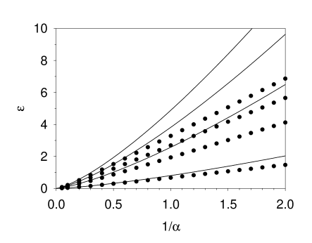
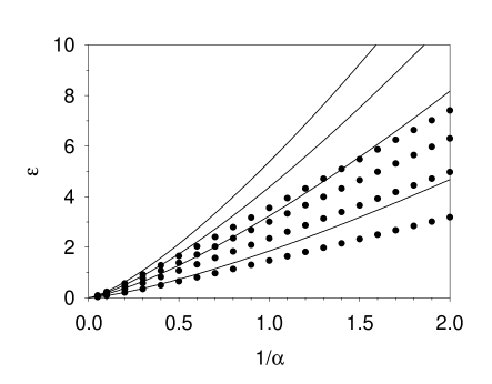
(a)	(b)

FIG. 1.: Lowest four eigenvalues $\varepsilon\equiv E/m-1$ for the scalar potential as functions of $1/\alpha\equiv\sqrt{g}/m$ for (a) even and (b) odd parity. The solid lines are the nonrelativistic results, and the points are positive-energy relativistic results.

From these results we see that the Dirac equation with a scalar linear potential is a well-defined problem in one dimension, with a rich set of solutions and a smooth nonrelativistic limit. As an exercise, one could extend this work to include calculation of the relativistic wave functions and make direct comparisons with the nonrelativistic Airy functions. They will match in the large-$\alpha$ limit. A second interesting exercise is a comparison of the ultrarelativistic, strong-coupling limit of the spectrum to the $\alpha^{-4/3}$ behavior of the nonrelativistic spectrum. The plots in Fig. 1 appear to imply a $\alpha^{-1}$ behavior for small $\alpha$.

REFERENCES

• [1] H. Galić, “Fun and frustration with hydrogen in a $1+1$ dimension,” Am. J. Phys. 56 (4), 312-317 (1988).
• [2] A. Z. Capri and R. Ferrari, “Hydrogenic atoms in one-plus-one dimensions,” Can. J. Phys. 63, 1029-1031 (1985).
• [3] R. S. Bhalerao and B. Ram, “Fun and frustration with quarkonium in a $1+1$ dimension,” Am. J. Phys. 69 (7), 817-818 (2001).
• [4] See also A. S. de Castro, quant-ph/0110178, which became available after the present work was completed.
• [5] The tildes are used to distinguish this representation from the one used in Ref. [IV].
• [6] M. Abramowitz and I. A. Stegun, Handbook of Mathematical Functions (Dover, New York, 1972).
• [7] F. A. B. Coutinho, Y. Nogami, and F. M. Toyama, “General aspects of the bound-state solutions of the one-dimensional Dirac equation,” Am. J. Phys. 56 (10), 904-907 (1988).
• [8] N. N. Lebedev, Special Functions and their Applications (Dover, New York, 1972), p. 294.
• [9] The usual solution of odd-order Hermite polynomials for the half-harmonic oscillator, where $V=\frac{1}{2}m\omega^{2}x^{2}$ for $x>0$ but is infinite for $x<0$, is correct because the solutions to $H_{\nu}(0)=0$ are the odd integers, not because $\nu$ is first restricted to being an integer by boundary conditions.
• [10] J. D. Bjorken and S. D. Drell, Relativistic Quantum Mechanics (McGraw-Hill, New York, 1964), p. 24.