Adaptive quantum measurements of a continuously varying phase

Abstract

We analyze the problem of quantum-limited estimation of a stochastically varying phase of a continuous beam (rather than a pulse) of the electromagnetic field. We consider both nonadaptive and adaptive measurements, and both dyne detection (using a local oscillator) and interferometric detection. We take the phase variation to be $\dot{\varphi}=\sqrt{\kappa}\xi(t)$, where $\xi(t)$ is $\delta$-correlated Gaussian noise. For a beam of power $P$, the important dimensionless parameter is $N=P/\hbar\omega\kappa$, the number of photons per coherence time. For the case of dyne detection, both continuous-wave (cw) coherent beams and cw (broadband) squeezed beams are considered. For a coherent beam a simple feedback scheme gives good results, with a phase variance $\simeq N^{-1/2}/2$. This is $\sqrt{2}$ times smaller than that achievable by nonadaptive (heterodyne) detection. For a squeezed beam a more accurate feedback scheme gives a variance scaling as $N^{-2/3}$, compared to $N^{-1/2}$ for heterodyne detection. For the case of interferometry only a coherent input into one port is considered. The locally optimal feedback scheme is identified, and it is shown to give a variance scaling as $N^{-1/2}$. It offers a significant improvement over nonadaptive interferometry only for $N$ of order unity.

I Introduction

The phase of an electromagnetic field is not a quantity that can be directly measured. All phase-measurement schemes rely on measurement of some other quantity, which necessarily introduces an excess uncertainty in the phase estimate. The standard method of measuring the phase of a single mode is to combine it with a strong local-oscillator field, which is detuned from the signal (so the phase changes linearly with respect to the signal phase). This is called the heterodyne scheme, and introduces an excess uncertainty scaling as $1/\overline{n}$, where $\overline{n}$ is the mean photon number. If the signal phase is known approximately beforehand, the introduced phase uncertainty can be reduced greatly by using a local-oscillator phase that is $\pi/2$ out of phase with the signal (homodyne measurements).

If there is no estimate for the phase available beforehand, it is still possible to reduce the excess phase uncertainty by adjusting the local-oscillator phase during the measurement so as to approximate a homodyne measurement Wis95c ; semiclass ; fullquan . The mark II dyne measurements considered in Refs. semiclass and fullquan introduce an excess phase uncertainty scaling as $\overline{n}^{-3/2}$. It is even possible to attain the theoretical limit, scaling as $\ln\overline{n}/\overline{n}^{2}$, using a more sophisticated feedback scheme unpub .

The case of interferometry is quite similar. In interferometry we wish to measure the phase shift in one arm of an interferometer by counting photons in the output ports. If a phase shift varying linearly in time is introduced into the other arm (analogous to the heterodyne case), there is a large introduced phase variance scaling as $\bar{n}^{-1}$. On the other hand, if feedback is used to adjust the auxiliary phase shift adaptively, the introduced phase variance is greatly reduced short ; long .

These studies are all based on single-shot measurements, where the measurements are made on a single (one- or two-mode) pulse with finite duration and a single fixed phase. In practice, if we wish to transmit information via a beam, a time-varying phase would be more convenient. A time-varying phase may also arise through random fluctuations, and we may wish to keep track of the phase as well as possible.

It is also possible to model a broadband signal that carries information by random fluctuations. We therefore consider the case of a phase subject to white noise in this paper. We consider cw measurements for both dyne measurements and interferometry. For the former, we consider both coherent beams and broadband squeezed beams. For interferometry it is not clear if there is a cw analog to the optimal two-mode states derived in Refs. short ; long . Therefore, we consider only the case of a coherent input into one port.

II Adaptive Dyne Measurements on a Coherent Beam

First, we will consider the case of cw dyne measurements on a single beam with a varying phase. It is simplest to consider a coherent beam with amplitude $\alpha=|\alpha|\exp[i\varphi(t)]$ having a constant magnitude, but varying phase. The magnitude is scaled so that $|\alpha|^{2}$ is the photon flux ($P/\hbar\omega$). As explained above, the phase is assumed to diffuse in time,

$$\varphi(t+dt)=\varphi(t)+\sqrt{\kappa}dW^{\prime}(t).$$ (1)

Here $dW^{\prime}$ is a Wiener increment satisfying $(dW^{\prime})^{2}=dt$. The spectrum for the coherent beam is a Lorentzian of linewidth (full width at half maximum) $\kappa$.

As in the single-shot case, a quadrature of the field is measured by combining the mode to be measured with a large-amplitude local-oscillator field at a 50:50 beam splitter and measuring the outputs with photodetectors. The photocurrent is then defined by

$$I(t)=\lim_{\delta t\to 0}\lim_{\beta\to\infty}\frac{\delta N_{+}-\delta N_{-}}{\beta\delta t},$$ (2)

where $\delta N_{+}$ and $\delta N_{-}$ are the outputs from the photodetectors and $\beta$ is the local-oscillator amplitude. For a continuous coherent beam this yields

$$I(t)dt=2{\rm Re}(\alpha e^{-i\Phi(t)})dt+dW(t),$$ (3)

where $\Phi(t)$ is the phase of the local oscillator, and $dW(t)$ is a Wiener increment independent of $dW^{\prime}(t)$.

In making adaptive phase measurements the phase of the local oscillator is usually taken to be $\Phi(t)=\hat{\varphi}(t)+\pi/2$, where $\hat{\varphi}(t)$ is some estimate of the system phase $\varphi(t)$ fn1 . With this, the signal becomes

$$I(t)dt=2|\alpha|\sin\left[\varphi(t)-\hat{\varphi}(t)\right]dt+dW(t).$$ (4)

II.1 Linear Approximation

Provided that the estimated system phase is sufficiently close to the actual system phase, we can make the linear approximation

$$I(t)dt=2|\alpha|[{\varphi(t)-\hat{\varphi}(t)}]dt+dW(t).$$ (5)

Rearranging this equation, we see that

$$\theta(t)={\hat{\varphi}(t)+{I(t)}/{2\left|\alpha\right|}}$$ (6)

is an unbiased estimator of $\varphi(t)$ based on the data obtained in the infinitesimal time interval $[t,t+dt)$. We will denote the best phase estimate based on all the data up to time $t$ by $\Theta(t)$. Note that this is the best phase estimate, in contrast to the phase estimate used in the feedback $\hat{\varphi}(t)$. The variance of each phase estimate $\theta(t)$ is given by

$$\langle{[\theta(t)-\varphi(t)]^{2}}\rangle=\left\langle{\left({\frac{dW(t)}{2|\alpha|dt}}\right)^{2}}\right\rangle=\frac{1}{4|\alpha|^{2}dt}.$$ (7)

Here the simple definition of the variance has been used, rather than the Holevo phase variance Hol84

$$V_{H}(\Theta)=|\langle{e^{i\Theta}}\rangle|^{-2}-1,$$ (8)

as in Refs. semiclass ; fullquan ; unpub ; short ; long . This is because we are using the linear approximation.

The noise in the estimate $\theta(t)$ is due entirely to the photocurrent noise, rather than the noise in the phase $\varphi$ itself. Since $dW(t)$ is independent of all previous noise, the updated best estimate $\Theta(t+dt)$ will be a weighted average of the instantaneous phase estimate $\theta(t)$ and the estimate from all the previous data $\Theta(t)$.

The equilibrium value of the variance of $\Theta(t)$, with all the individual phase estimates correctly weighted, will be denoted by $\Delta\Theta^{2}$. From Eq. (1), after a time $dt$ the phase variance of $\Theta(t)$ with respect to the new system phase $\varphi(t+dt)$ will be $\Delta\Theta^{2}+\kappa dt$. The variance in the phase estimate from the latest time interval, $\theta(t)$, will be given by Eq. (7).

If we take a weighted average of $\Theta(t)$ and $\theta(t)$, then the contributions from each of the phase estimates from the individual time intervals should be correctly weighted, and the variance in the weighted average should be the equilibrium value, $\Delta\Theta^{2}$. This implies that

$${\frac{1}{{\Delta\Theta^{2}+\kappa dt}}+4|\alpha|^{2}dt}=\frac{1}{\Delta\Theta^{2}}.$$ (9)

Solving for $\Delta\Theta^{2}$ gives $\Delta\Theta^{2}=\sqrt{\kappa}/{2|\alpha|}$. If we define

$$N=|\alpha|^{2}/\kappa,$$ (10)

the number of photons per coherence time (or photon flux divided by linewidth), we have

$$\Delta\Theta^{2}={1}/{2\sqrt{N}}.$$ (11)

This is the square root of the analogous result $1/4\bar{n}$ for a single-shot adaptive measurement on a coherent pulse of mean photon number $\bar{n}$.

Explicitly, the weighted average is

$$\Theta(t+dt)=\frac{({4|\alpha|^{2}dt})\theta(t)+\Theta(t)/(\Delta\Theta^{2}+\kappa dt)}{1/{\Delta\Theta^{2}}}.$$ (12)

Solving this as a differential equation gives

$$\Theta(t)=2|\alpha|\sqrt{\kappa}\int_{-\infty}^{t}{\theta(s)e^{2|\alpha|\sqrt{\kappa}(s-t)}ds}.$$ (13)

Therefore, this method corresponds to a simple negative exponential scaling of the weighting.

We can also consider a more general negative exponential scaling given by

$$\Theta(t)=\chi\int_{-\infty}^{t}{\theta(s)e^{\chi(s-t)}ds}.$$ (14)

Note that with this more general scaling, $\Theta(t)$ is no longer necessarily the best phase estimate. For most of the remainder of this paper, $\Theta(t)$ will be used in this more general sense, rather than as specifically the best phase estimate. The best phase estimate will be found by finding the optimum value of $\chi$. Taking the derivative of this expression with respect to time gives

$$\Theta(t+dt)=\chi dt\theta(t)+(1-\chi dt)\Theta(t).$$ (15)

This means that this method is again a weighted average, except with a weighting that is not optimum. If we find the variance of both sides of this equation and solve for $\Delta\Theta^{2}$ we obtain

$$\Delta\Theta^{2}=\frac{\chi}{8|\alpha|^{2}}+\frac{\kappa}{2\chi}.$$ (16)

This equation has a minimum of $\Delta\Theta^{2}=\sqrt{\kappa}/2|\alpha|$ for $\chi=2|\alpha|\sqrt{\kappa}$, reproducing the result found more directly above.

II.2 Exact treatment

The results of the previous section are all using the linear approximation (5). Although this approximation is very useful for obtaining the asymptotic value of the variance, it does not directly tell us what to do in the exact case. In the exact case for single-shot measurements semiclass , rather than averaging phase estimates from each time interval, we determine $A_{v}$ and $B_{v}$, defined (for scaled time $v\in[0,1]$) as

$$A_{v}=\int_{0}^{v}{e^{i\Phi}I(u)du},~{}~{}~{}B_{v}=-\int_{0}^{v}{e^{2i\Phi}du},$$ (17)

and obtain the phase estimate from

$$\Theta(v)=\arg\left(vA_{v}+B_{v}A_{v}^{*}\right).$$ (18)

The intermediate phase estimate in the simplest (mark II) case semiclass was

$$\hat{\varphi}(v)=\arg A_{v}.$$ (19)

We seek cw analogues of these formulas, that should reproduce the above linearized results in the appropriate (large $N$) regime. Guided by Sec. II.1, we replace the definitions of $A_{v}$ and $B_{v}$ by

$$A_{t} =\int_{-\infty}^{t}e^{\chi(u-t)}e^{i\Phi}I\left(u\right)du,$$ (20)

$$B_{t} =-\int_{-\infty}^{t}e^{\chi(u-t)}e^{2i\Phi}du,$$ (21)

and continue to use $\arg A_{t}$ as the intermediate phase estimate $\hat{\varphi}(t)$. We will not consider any better intermediate phase estimates here, as these only give very small improvements over the mark II case for coherent states.

To find a formula for $\Theta(t)$, we can use a similar approach to that used in Ref. semiclass . Let us ignore the variation of the system phase in Eq. (20). Since we expect from Sec. II.1 that for large $N$ the optimal $\chi$ is ${\rm O}(|\alpha|\sqrt{\kappa})={\rm O}(\kappa\sqrt{N})\gg\kappa$, this is a reasonable approximation. Then we find

$$A_{t}={\alpha}/{\chi}-\alpha^{*}B_{t}+i\sigma_{t},$$ (22)

where

$$\sigma_{t}=\int_{-\infty}^{t}e^{\chi(u-t)}e^{i\left(\Phi-\pi/2\right)}dW(u).$$ (23)

Equation (22) is analogous to the corresponding result semiclass for the case of single-shot measurements, except with $v$ replaced with $1/\chi$. Note that from this derivation it naturally emerges that we should use the same exponential in the integrand for $B_{t}$ as for $A_{t}$. From Eq. (22) it can be shown that

$$A_{t}+\chi B_{t}A_{t}^{*}=\alpha(1/\chi-\chi|B_{t}|^{2})+i\sigma_{t}-i\chi B_{t}\sigma_{t}^{*}.$$ (24)

Taking the expectation value gives

$$\left\langle{A_{t}+\chi B_{t}A_{t}^{*}}\right\rangle\approx\alpha(1/\chi-\chi|B_{t}|^{2}).$$ (25)

If the local oscillator phase is independent of the photocurrent record, then this is exact. In the case of feedback, $B_{t}$ may be correlated with $\sigma_{t}$, but this result should still be approximately true. Therefore, the phase estimate that will be used here is

$$\Theta(t)=\arg(A_{t}+\chi B_{t}A_{t}^{*}).$$ (26)

Similarly to the single-shot case unpub , we will define the variable $C_{t}=A_{t}+\chi B_{t}A_{t}^{*}$, so $\Theta(t)=\arg C_{t}$. The above derivation is not exact if the system phase is not constant; however, $\arg C_{t}$ should still be a good estimator for the phase in the semiclassical limit.

A differential equation for the feedback phase can be determined in a similar way as in Ref. semiclass . Using Eq. (20), we can determine the increment in $A_{t}$,

$$dA_{t}=e^{i\Phi}I(t)dt-\chi A_{t}dt.$$ (27)

Taking the local oscillator phase to be $\Phi(t)=\arg A_{t}+\pi/2$, we find that

$$dA_{t}=i\frac{A_{t}}{|A_{t}|}I(t)dt-\chi A_{t}dt,$$ (28)

so the magnitude of $A_{t}$ varies as

$$d|A_{t}|^{2} =A_{t}^{*}\left(dA_{t}\right)+\left(dA_{t}^{*}\right)A_{t}+\left(dA_{t}^{*}\right)\left(dA_{t}\right)$$

$$=\left(1-2\chi|A_{t}|^{2}\right)dt.$$ (29)

Thus $|A_{t}|$ increases up to an equilibrium value given by $|A_{t}|^{2}=1/2\chi$.

Using this result, the increment in the feedback phase in the steady state is

$$d\Phi(t) ={\rm Im}[d\ln A_{t}]$$

$$={\rm Im}\left[\frac{dA_{t}}{A_{t}}-\frac{\left(dA_{t}\right)^{2}}{2A_{t}^{2}}\right]$$

$$=\frac{I(t)dt}{|A_{t}|}=\sqrt{2\chi}I(t)dt.$$ (30)

Therefore, the feedback phase just changes linearly with the signal, with constant coefficient (rather than a time-dependent coefficient as in the pulsed case semiclass ).

Using this result gives the stochastic differential equation for the phase estimate $\hat{\varphi}(t)$ as

$$d\hat{\varphi}(t)=\sqrt{2\chi}\{2|\alpha|\sin[\varphi(t)-\hat{\varphi}(t)]dt+dW(t)\}.$$ (31)

Making a linear approximation gives

$$d\hat{\varphi}(t)=\sqrt{2\chi}\{2|\alpha|[\varphi(t)-\hat{\varphi}(t)]dt+dW(t)\}.$$ (32)

Rearranging and integrating then gives the solution as

$$\hat{\varphi}(t)=\sqrt{2\chi}\int_{-\infty}^{t}e^{2|\alpha|\sqrt{2\chi}(u-t)}\left[2|\alpha|\varphi(u)du+dW(u)\right].$$ (33)

If the phase is measured relative to the current system phase, then

$$\varphi(u)=-\sqrt{\kappa}\int_{u}^{t}dW^{\prime}(s).$$ (34)

To determine an expression for the phase estimate $\Theta(t)$, note that it can be simplified to

$$\Theta(t)=\hat{\varphi}(t)+\arg(1+\chi e^{-2i\hat{\varphi}(t)}B_{t}).$$ (35)

Using Eq. (21) and expanding the exponentials to first order gives

$$\Theta(t) \approx\hat{\varphi}(t)+\arg\left(1-i\hat{\varphi}(t)+i\chi\int_{-\infty}^{t}e^{\chi(u-t)}\hat{\varphi}(u)du\right)$$

$$\approx\chi\int_{-\infty}^{t}\hat{\varphi}(u)e^{\chi(u-t)}du.$$ (36)

This demonstrates that the mark II phase estimate is approximately a weighted average of the intermediate phase estimates, just as in the pulsed case it is approximately an unweighted average semiclass . Note also the similarity of this result to the result for the linear case (14). Unfortunately the simple technique used in the linear case cannot be applied here. However, using the standard techniques of stochastic calculus, the expectation value $\langle\Theta^{2}(t)\rangle$ can be determined from Eq. (36), in a lengthy but straightforward calculation. The result is exactly the same as that obtained using the linear approximation (16).

III Heterodyne Measurements on a Coherent Beam

In order to determine how much of an improvement feedback gives for cw measurements, we will compare it with the case of cw heterodyne measurements. For heterodyne measurements on a pulsed coherent state, the introduced phase variance is equal to the intrinsic phase variance. This indicates that the first term in Eq. (16) should be double for the heterodyne case, so the phase variance is

$$\left\langle{\Theta^{2}(t)}\right\rangle\approx\frac{\chi}{4|\alpha|^{2}}+\frac{\kappa}{2\chi}.$$ (37)

We now show this more rigorously using a similar technique to that used in Ref. semiclass . Expanding $A_{t}$ gives

$$A_{t}=\int_{-\infty}^{t}e^{\chi(u-t)}e^{i\Phi(u)}[(\alpha e^{-i\Phi}+\alpha^{*}e^{i\Phi})du+dW(u)].$$ (38)

For the heterodyne case, the local oscillator phase $\Phi(t)$ varies very rapidly, so the second term above will be negligible. This means that $A_{t}$ simplifies to

$$A_{t}=|\alpha|\int_{-\infty}^{t}e^{\chi(u-t)}e^{i\varphi(u)}du+i\sigma_{t}.$$ (39)

Since $B_{t}$ is also negligible, the phase estimate $\Theta(t)$ simplifies to $\Theta(t)=\arg A_{t}$. As above, the phase will be measured relative to the current system phase. In the limit $N\gg 1$, the system phase does not vary significantly during the time $1/\chi$, so we can take the linear approximation, giving

$$A_{t}\approx\frac{|\alpha|}{\chi}+i|\alpha|\int_{-\infty}^{t}e^{\chi(u-t)}\varphi(u)du+i\sigma_{t}.$$ (40)

Using this, the phase estimate is

$$\Theta(t)\approx{\rm Im}\left[i\chi\int_{-\infty}^{t}e^{\chi(u-t)}\varphi(u)du+i\chi\sigma_{t}/|\alpha|\right].$$ (41)

Here the linear approximation has again been used. Further evaluating this gives

$$\Theta(t)=-\sqrt{\kappa}\chi\int_{-\infty}^{t}\!\!\!du\,e^{\chi(u-t)}\int_{u}^{t}dW^{\prime}(s)+\frac{\chi}{2|\alpha|}(\sigma_{t}+\sigma_{t}^{*}).$$ (42)

The variance is, therefore,

$$\langle{\Theta^{2}(t)}\rangle =\kappa\chi^{2}\left\langle\int_{-\infty}^{t}du_{1}\int_{-\infty}^{t}du_{2}e^{\chi(u_{1}+u_{2}-2t)}\right.$$

$$~{}~{}~{}\left.\times\int_{u_{1}}^{t}dW^{\prime}(s_{1})\int_{u_{2}}^{t}dW^{\prime}(s_{2})\right\rangle$$

$$~{}~{}~{}+\frac{\chi^{2}}{4|\alpha|^{2}}\left\langle{(\sigma_{t}+\sigma_{t}^{*})^{2}}\right\rangle.$$ (43)

The first term here can be evaluated to give ${\kappa}/{2\chi}$. In addition, it is easy to show that $\langle{\sigma_{t}^{2}}\rangle\approx 0$ and $\langle{|\sigma_{t}|^{2}}\rangle=1/{2\chi}$. Using these results gives the variance as

$$\left\langle{\Theta^{2}(t)}\right\rangle=\frac{\kappa}{2\chi}+\frac{\chi}{4|\alpha|^{2}}.$$ (44)

This shows that Eq. (37) is correct. Using this result, the minimum variance is ${\sqrt{\kappa}}/{\sqrt{2}|\alpha|}$ for $\chi=\sqrt{2\kappa}|\alpha|$. In terms of $N$, this is $1/\sqrt{2N}$, which is $\sqrt{2}$ times the minimum phase variance for the adaptive case.

IV Results for Dyne Measurements on a Coherent Beam

In order to verify the above analytical results, the equilibrium phase variance was determined numerically for a variety of parameters. Because we do not presuppose a value for $\chi$, there are two dimensionless parameters in our simulations,

$$N=\frac{|\alpha|^{2}}{\kappa},~{}~{}~{}{\rm X}=\frac{\chi}{|\alpha|^{2}}.$$ (45)

From the above theory, the optimum value of ${\rm X}$ is $2/\sqrt{N}$ for the adaptive case and $\sqrt{2/N}$ for the heterodyne case.

The value of $N$ was varied from 1 up to $2.5\times 10^{37}$. For each value of $N$, ${\rm X}$ was varied from a quarter to four times $2/\sqrt{N}$. Measuring time in units of $|\alpha|^{-2}$, the time steps used were $\Delta t=1/10^{3}{\rm X}$. For these calculations 1024 simultaneous integrations were performed and the variance was sampled repeatedly. The integrations were taken up to time $10/{\rm X}$, in order for the variance to reach its equilibrium value, then the variance was sampled at time intervals of $1/{\rm X}$ up until time $100/{\rm X}$.

The results for ${\rm X}=2/\sqrt{N}$ are plotted in Fig. 1. The variances for $N=1$ to $4\times 10^{12}$ are the Holevo variances, and for above $4\times 10^{12}$ are the standard variances. As can be seen, the results are very close to the theoretical values. To show the improvement over heterodyne measurements, the ratio of the minimum phase variance for adaptive measurements to the minimum phase variance for heterodyne measurements (with ${\rm X}=\sqrt{2/N}$) is plotted in the inset of Fig. 1. The ratio is close to 1 for small $N$, but for larger $N$ the ratio gets closer and closer to $1/\sqrt{2}$.

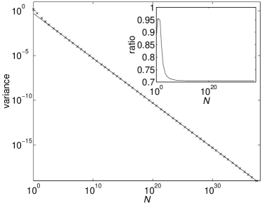
Figure 1: The phase variance for cw adaptive measurements for ${\rm X}=2/\sqrt{N}$. The numerical results are shown as crosses and the theoretical values of $1/\sqrt{2N}$ are shown as the continuous line. The inset shows the ratio of the minimum phase variance for cw adaptive measurements to the minimum phase variance for cw heterodyne phase measurements.

Alternatively we can plot the phase variance as a function of ${\rm X}$ for fixed $N$. In Fig. 2 we have shown the phase variance as a function of ${\rm X}$ for $N=10^{6}$, for adaptive and heterodyne measurements. The numerical results agree reasonably closely with the theoretical values, although there is a noticeable difference for adaptive measurements for the larger values of ${\rm X}$. Note that the minimum phase variance for adaptive measurements is at ${\rm X}=2/\sqrt{N}$, and the minimum phase variance for heterodyne measurements is larger and at a smaller value of ${\rm X}$. When the value of $N$ is increased further, the numerical results agree even more closely with the theoretical values.

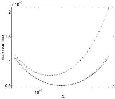
Figure 2: The phase variance as a function of ${\rm X}$ for $N=10^{6}$. The numerical results for adaptive and heterodyne measurements are shown as the crosses and pluses, respectively, and the theoretical results for adaptive and heterodyne measurements are shown as the continuous line and dotted line, respectively.

V Adaptive Dyne Measurements on a Broadband Squeezed Beam

The above results show that the improvement offered by adaptive measurements over nonadaptive (heterodyne) measurements in the case of a coherent beam is only a factor of $1/\sqrt{2}$ reduction in the variance. This is similar to the single-shot case, where a $1/2$ reduction was found for the coherent case. However, in the single-shot case a far more dramatic reduction is found for the case of a squeezed state. Motivated by this we now consider adaptive dyne measurements on a cw squeezed beam.

It is simplest to consider broadband squeezing. Physically, this could arise as the output of a driven parametric oscillator in the limit that the decay time of the cavity is much shorter than any other relevant timescales Gar91 . This results in the modification of the photocurrent from Eq. (3) to

$$I(t)dt =2{\rm Re}(\alpha e^{-i\Phi(t)})dt+dW(t)$$

$$~{}~{}~{}\times\sqrt{e^{-2r}\cos^{2}(\Phi-\phi_{\zeta}/2)+e^{2r}\sin^{2}(\Phi-\phi_{\zeta}/2)},$$ (46)

where $\alpha$ is the amplitude of the squeezed beam, and $r$ and $\phi_{\zeta}$ are the magnitude and phase of the squeezing, respectively. In this idealized limit the noise reduction via squeezing occurs by a reduction in the shot noise level, rather than an anticorrelation between the shot noise and the later coherent amplitude (as in the single-shot case).

For reduced phase uncertainty, the phase of the squeezing should be $\phi_{\zeta}=2\varphi+\pi$, where $\varphi$ is the system phase. If we are using feedback given by $\Phi=\hat{\varphi}+\pi/2$, where $\hat{\varphi}$ is an estimate of the phase, then the photocurrent can be expressed as

$$I(t)dt =2|\alpha|\sin(\varphi-\hat{\varphi})dt$$

$$~{}~{}~{}+dW(t)\sqrt{e^{-2r}\cos^{2}(\hat{\varphi}-\varphi)+e^{2r}\sin^{2}(\hat{\varphi}-\varphi)}.$$ (47)

It is clear that if the intermediate phase estimate used is very close to the system phase, then the factor multiplying $dW$ will be close to $e^{-r}$ and will be at a minimum. The better the intermediate phase estimate is, the smaller this multiplying factor will be. If the intermediate phase estimate is not perfect, it is clear that increasing the squeezing past a certain level will not reduce the multiplying factor. This is because the $e^{2r}$ term will start to dominate.

It is possible to estimate the optimum squeezing and the minimum phase variance using the linear approximation. In this approximation, the variance in the individual phase estimates $\theta(t)$ is

$$[{e^{-2r}\cos^{2}(\hat{\varphi}-\varphi)+e^{2r}\sin^{2}(\hat{\varphi}-\varphi)}]/{4|\alpha|^{2}dt}.$$ (48)

It is clear that the minimum phase variance (in this approximation) will be obtained when the best phase estimates are used for $\hat{\varphi}$. It is therefore reasonable to use the phase estimates $\Theta(t)$ for $\hat{\varphi}$, rather than $\arg A_{t}$ as in the coherent case. The values of $\Theta(t)$ will be the best phase estimates when the correct $\chi$ is used. As the variance of these estimates is $\Delta\Theta^{2}$, we obtain

$$\langle{e^{-2r}\cos^{2}(\hat{\varphi}-\varphi)+e^{2r}\sin^{2}(\hat{\varphi}-\varphi)}\rangle\approx e^{-2r}+e^{2r}\Delta\Theta^{2}.$$ (49)

This approximation will be true for small phase variances and large squeezing. Following the same derivation as for the coherent case, the only difference is the multiplying factor, so we obtain

$$\Delta\Theta^{2}=\frac{\chi}{8|\alpha|^{2}}\left(e^{-2r}+e^{2r}\Delta\Theta^{2}\right)+\frac{\kappa}{2\chi}.$$ (50)

This expression has two independent variables, $\chi$ and $r$, that can be varied in order to find the minimum phase variance. Taking the derivative of Eq. (50) with respect to $\chi$ and setting the result to zero gives

$$\chi=\frac{\kappa}{\Delta\Theta^{2}}.$$ (51)

Substituting this into Eq. (50) gives

$$\Delta\Theta^{2}=\frac{\kappa}{4|\alpha|^{2}}\left(e^{2r}+\frac{e^{-2r}}{\Delta\Theta^{2}}\right).$$ (52)

Taking the derivative of this with respect to $r$ and again setting the result equal to zero gives

$$e^{-4r}=\Delta\Theta^{2}.$$ (53)

Substituting this back into Eq. (52) gives the phase variance as

$$\Delta\Theta^{2}=\left(\frac{\kappa}{2|\alpha|^{2}}\right)^{2/3}=\left(\frac{1}{2N}\right)^{2/3}.$$ (54)

Thus we see that even for an arbitrarily squeezed beam, the best scaling we can obtain for the phase variance is $N^{-2/3}$, as compared to $N^{-1/2}$ for a coherent beam. This difference is less than for pulsed measurements, where the phase variance for the optimum squeezed states scales almost as $\overline{n}^{-2}$, as compared to $\overline{n}^{-1}$ for coherent states.

VI Heterodyne Measurements on a Broadband Squeezed Beam

In order to determine the phase variance for heterodyne measurements on a squeezed beam, we can simply perform the derivation of Sec. III, except with the factor multiplying $dW$ from Eq. (V) included. This means that the variance will be

$$\langle{\Theta^{2}(t)}\rangle=\frac{\kappa}{2\chi}+\frac{\chi^{2}}{4|\alpha|^{2}}\langle{(\sigma_{t}+\sigma_{t}^{*})^{2}}\rangle,$$ (55)

except with $\sigma_{t}$ modified to

$$\sigma_{t} =\int_{-\infty}^{t}e^{\chi(u-t)}e^{i\left(\Phi-\pi/2\right)}$$

$$~{}~{}~{}\times\sqrt{e^{-2r}\sin^{2}(\Phi-\varphi)+e^{2r}\cos^{2}(\Phi-\varphi)}dW(u).$$ (56)

Here we have used the assumption that the phase of the squeezing is $2\varphi+\pi$. Note that the derivation of Sec. III takes the phase relative to the current system phase. This means that to a first approximation we may take $\varphi(u)=0$.

In order to determine the phase variance, we must determine the expectation values $\langle{|\sigma_{t}|^{2}}\rangle$ and $\langle{\sigma_{t}^{2}}\rangle$. We find

$$\langle{|\sigma_{t}|^{2}}\rangle=\int_{-\infty}^{t}e^{2\chi(u-t)}\left(e^{-2r}\sin^{2}\Phi+e^{2r}\cos^{2}\Phi\right)du.$$ (57)

As the local oscillator phase $\Phi$ is varying rapidly in the heterodyne case, we may take the average values of $\sin^{2}$ and $\cos^{2}$, giving

$$\langle{|\sigma_{t}|^{2}}\rangle=\frac{\cosh(2r)}{2\chi}.$$ (58)

Similarly, evaluating $\langle{\sigma_{t}^{2}}\rangle$ gives

$$\langle{\sigma_{t}^{2}}\rangle=-\int_{-\infty}^{t}e^{2\chi(u-t)}e^{2i\Phi}\left(e^{-2r}\sin^{2}\Phi+e^{2r}\cos^{2}\Phi\right)du.$$ (59)

Taking trigonometric averages as above gives

$$\langle{\sigma_{t}^{2}}\rangle=-\frac{\sinh(2r)}{4\chi}.$$ (60)

Using these results we obtain the phase variance as

$$\langle{\Theta^{2}(t)}\rangle=\frac{\kappa}{2\chi}+\frac{\cosh(2r)-\tfrac{1}{2}\sinh(2r)}{4|\alpha|^{2}/\chi}.$$ (61)

This differs from the result for the coherent case by the multiplying term $\cosh(2r)-\tfrac{1}{2}\sinh(2r)$. This has a minimum of $\sqrt{3}/2$ for $r=\ln(3)/4$. Using this value, we obtain the minimum variance as $3^{1/4}\sqrt{\kappa}/(2\alpha)$ for $\chi=2\sqrt{\kappa}|\alpha|/3^{1/4}$. Thus we find that the scaling is the same as for a coherent beam, and the multiplying factor is only about 7% smaller. In contrast there is a factor of two difference in the single-shot case.

VII Results for Dyne Measurements on a Broadband Squeezed Beam

The results for the cw squeezed beam were obtained by a similar method as for the coherent case. Only variation in the variables $N$ and ${\rm X}$ of Eq. (45) was considered, and time was measured in units of $|\alpha|^{-2}$. The step sizes used were $\Delta t={1}/{10^{3}{\rm X}}$. The integrations were taken up to time $30/{\rm X}$, then the variance was sampled every time step until time $130/{\rm X}$. The integration was performed using the photocurrent given in Eq. (V) with $\phi_{\zeta}=2\varphi+\pi$.

It was found that when $\hat{\varphi}(t)=\arg C_{t}$ was used in the feedback, very poor results were obtained. This is a similar result to the case for single-shot measurements, where using $\arg C_{v}$ feedback results in large phase variances unpub . This is because, when the intermediate phase estimates are extremely good, the results do not distinguish easily between the real system phase and the system phase plus $\pi$. This means that many of the results are out by $\pi$, resulting in a large overall phase variance.

In order to avoid this problem, rather than using $\arg C_{t}$ in the feedback, an intermediate phase estimate given by

$$\hat{\varphi}(t)=\arg(C_{t}^{1-\varepsilon}A_{t}^{\varepsilon})$$ (62)

was used, with $\varepsilon$ constant. Note that this is the same as used to obtain phase measurements close to optimum in the single-shot case, except that there a time-varying $\varepsilon$ was used.

For each value of $N$ there are three variables that can be altered to minimize the phase variance: ${\rm X}$, $r$, and $\varepsilon$. It is not calculationally feasible to consider a range of values for all three variables. Instead, different values were tried systematically to find the minimum phase variance.

The minimum phase variances obtained by this method are plotted as a function of $N$ in Fig. 3. The theoretical values given by Eq. (54) are also shown in this figure. The numerical results are higher than the theoretical values, but they have the same scaling with $N$, namely, $N^{-2/3}$. If we plot the ratio of the numerical results to the theoretical values as in the inset of Fig. 3, we find that for the largest values of $N$ the ratio levels off at about $2.6$.

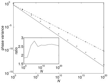
Figure 3: The phase variance as a function of $N$ for a cw squeezed beam. The theoretical relations for adaptive and heterodyne measurements are shown as the continuous line and dashed line respectively, and the numerical results for adaptive and heterodyne measurements are shown as the crosses and pluses respectively. The inset shows the ratio of the numerically obtained phase variance to the theoretical value as a function of $N$ for adaptive measurements.

Now note that, from Eqs. (53) and (54), the optimum value of $e^{-2r}$ should be $(2N)^{-1/3}$. Similarly, from Eqs. (51) and (54), the optimum value of ${\rm X}$ is $(N/4)^{-1/3}$. The numerically obtained optimum values of $e^{-2r}$ and ${\rm X}$, as well as these theoretical expressions, are plotted in Fig. 4. Similarly to the case for the phase variance, the scaling is the same as theoretically predicted, but the scaling constants are different. For the case of $e^{-2r}$, the optimum values are about eight times those theoretically predicted, whereas the values of ${\rm X}$ are around a third of those theoretically predicted.

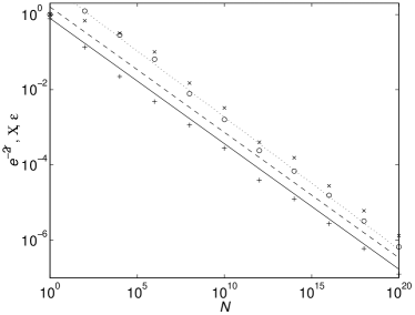
Figure 4: The optimum values of $e^{-2r}$, ${\rm X}$, and $\varepsilon$ for measurements on a cw squeezed beam. The numerically found values of $e^{-2r}$ are plotted as crosses, and the theoretical expression as a continuous line. The numerically found values of ${\rm X}$ are plotted as pluses, and the theoretical expression as a dashed line. The numerically found values of $\varepsilon$ are plotted as circles, and the dotted line is the expression fitted to the data.

For the case of $\varepsilon$ there is no theoretical prediction for the optimum value. The numerically obtained values are shown in Fig. 4, and as can be seen $\varepsilon$ decreases in a regular way with increasing $N$. A power law was fitted to these values (for $N>1$), and the power found was $-0.35\pm 0.01$. This is very similar to the $N^{-1/3}$ scaling found for $e^{-2r}$ and ${\rm X}$.

The results for heterodyne measurements are also shown in Fig. 3. The results in this case agree very accurately with the theoretical prediction, within about $0.5\%$ for the larger values of $N$. Similarly the optimum values of $r$ and $\chi$ agree very accurately with those predicted above. The variance scales as $N^{-1/2}$, in contrast to the variance for adaptive measurements that scales as $N^{-2/3}$. This means that the improvement in using adaptive measurements scales as $N^{-1/6}$, which can be very large for large $N$.

VIII cw Interferometry

Now we will turn from dyne measurement on a single beam to cw interferometric measurements. In this case we have a Mach-Zehnder interferometer (MZI), and are attempting to continuously track a stochastically varying phase in one arm, by controlling the phase in the other arm and detecting photons in the two output beams. This is shown in Fig. 5. In this context it is not possible to consider nonclassical states of the type considered for the single-shot case long . Instead, for simplicity, we will restrict our consideration to the case where all photons enter through one port. This can be realized using coherent light, with $|\alpha|^{2}$ photons per unit time. Note that because this is an interferometric measurement rather than one using a local oscillator as a phase reference, the phase of $\alpha$ is irrelevant.

Figure 5: The Mach-Zehnder interferometer, with the addition of a controllable phase $\Phi$ in one arm. The unknown phase to be estimated is $\varphi$. Both beam splitters are 50:50.

This case is essentially semiclassical, and the detections can be considered independently. Therefore, consider the state with a single photon incident on port $a$. The annihilation operators for the output modes of the MZI, $\hat{c}_{0}$ and $\hat{c}_{1}$, are related to the annihilation operators for the input modes, $\hat{a}$ and $\hat{b}$, by long

$$\hat{c}_{u}=\hat{a}\sin[(\varphi-\Phi+u\pi)/2]+\hat{b}\cos[(\varphi-\Phi+u\pi)/2],$$ (63)

for $u\in\{0,1\}$. Hence the probability for detecting the photon in detector $u$ is given by

$$\sin^{2}[(\varphi-\Phi+u\pi)/2].$$ (64)

Using Bayes’ theorem, the probability distribution for the system phase after the detection is proportional to this probability times the initial probability distribution.

Denote the results for $m$ such detections by the string $n_{m}=u_{m}u_{m-1}\cdots u_{1}$. The probability distribution for the phase given $n_{m}$, $P(\varphi|n_{m})$, can be expressed as

$$P(\varphi|n_{m})=\sum_{k=-m}^{m}P_{m;k}(n_{m})e^{ik\varphi}.$$ (65)

In the absence of any phase variation, it can be shown from Eq. (64) that the unnormalized coefficients $P^{\prime}_{m;k}(n_{m})$ can be determined by

$$P^{\prime}_{m;k}\!(n_{m}\!) \!=\!P_{m-1;k}\!(n_{m-1}\!)\!-\!\tfrac{1}{2}e^{-i(\Phi_{m}\!-u_{m}\pi)}\!P_{m-1;k-1}\!(n_{m-1}\!)$$

$$~{}~{}~{}-\tfrac{1}{2}e^{i(\Phi_{m}-u_{m}\pi)}P_{m-1;k+1}(n_{m-1}).$$ (66)

The normalization condition on the probability distribution becomes $P_{m;0}(n_{m})=1$. The normalized probability distribution can be obtained by simply dividing the coefficients obtained from Eq. (66) by $P^{\prime}_{m;0}(n_{m})$.

Similarly to the case of dyne measurements, we will assume that the system phase diffuses with time as in Eq. (1). When the phase varies in time, the time between detections is important. For a photon flux of $|\alpha|^{2}$, the probability of a photodetection in time $dt$ is $|\alpha|^{2}dt$. The probability distribution for the time between detections is given by the exponential distribution

$$P_{E}(t)dt=|\alpha|^{2}e^{-|\alpha|^{2}t}dt.$$ (67)

In the results that will be presented here, the time between detections, $\Delta t$, was determined according to this probability distribution.

Now in order to determine the effect of this phase diffusion on the probability distribution between detections, we must first consider the effect over some very small time interval $\delta t$. This is necessary because the probability distribution for the change in the system phase over time $\Delta t$ does not go to zero for $\Delta\varphi=\pm\pi$. This means that the probability distribution will not be exactly Gaussian, due to the overlap. In contrast, if we look at a very small time interval $\delta t$, the change in the phase will have a normal distribution with a variance of $\kappa\delta t$. Explicitly the probability distribution is

$$P_{G}(\Delta\varphi)d(\Delta\varphi)=\frac{1}{\sqrt{2\pi\kappa\delta t}}e^{-\Delta\varphi^{2}/(2\kappa\delta t)}d(\Delta\varphi).$$ (68)

The probability distribution for the phase after time $\delta t$ will be the convolution of the initial probability distribution with the Gaussian described by Eq. (68). Evaluating this convolution gives

$$P^{\delta t}(\varphi|n_{m}) =\int_{-\pi}^{\pi}P(\varphi-\theta|n_{m})P_{G}(\theta)d\theta$$

$$=\sum_{k=-m/2}^{m/2}P_{m;k}(n_{m})e^{ik\varphi}\int_{-\pi}^{\pi}e^{-ik\theta}P_{G}(\theta)d\theta.$$ (69)

As $\delta t$ is assumed to be small, $\kappa\delta t\ll 1$, and the integral in Eq. (69) evaluates to $e^{-k^{2}\kappa\delta t/2}$. The effect of the variation of the system phase on the probability distribution is, therefore,

$$P_{m;k}^{\delta t}(n_{m})=P_{m;k}(n_{m})e^{-k^{2}\kappa\delta t/2}.$$ (70)

In order to take account of the effect of the phase diffusion on the probability distribution over some significant time interval $\Delta t$, this time interval can be thought of as comprising $M$ small time intervals $\delta t$. Then we find that the coefficients are just multiplied by $M$ terms of $e^{-k^{2}\kappa\delta t/2}$. This is equivalent to a single term of $e^{-k^{2}\kappa\Delta t/2}$, which is very easy to implement.

As time passes the effect of Eq. (66) is to broaden the distribution of probability coefficients in $k$, corresponding to a smaller variance in the phase distribution. In contrast, the Gaussian term in Eq. (70) tends to narrow the distribution of probability coefficients, corresponding to a greater phase variance. The initially broad phase distribution narrows until an approximate equilibrium is reached, where the two effects cancel each other out.

In Ref. long it was shown that the optimum phase estimate for the single-shot case is

$$\Theta=\arg\langle{e^{i\varphi}}\rangle=\arg P_{m;-1}(n_{m}).$$ (71)

It is easy to see that this phase estimate is optimal in the cw case also. In addition we consider feedback that is equivalent to that considered in the single-shot case in Ref. long . Rather than using an intermediate phase estimate as in the dyne case, we use the full power of Bayesian statistics to choose the feedback phase $\Phi$ so as to minimize the expected Holevo phase variance after the next detection. This is achieved by choosing $\Phi_{m}$ to minimize the value of long ; thesis

$$M(\Phi_{m})=\sum_{u_{m}=0,1}\left|\int_{-\pi}^{\pi}P(n_{m}|\varphi)e^{i\varphi}d\varphi\right|.$$ (72)

The values of $P(n_{m}|\varphi)$ can be obtained, except for a normalizing constant that is common to $u_{m}=0$ and 1, by using Eq. (66). This means that we can express $M(\Phi_{m})$ as in Ref. long with the parameters $a$, $b$, and $c$ given by

$$a =P_{m-1;-1}(n_{m-1}),$$

$$b =\tfrac{1}{2}P_{m-1;-2}(n_{m-1}),$$

$$c =\tfrac{1}{2}P_{m-1;0}(n_{m-1}).$$ (73)

These values of $a$, $b$, and $c$ can be used to determine the feedback phase as in Ref. long .

The phase uncertainty at equilibrium can be estimated using a similar approach as was used for the single-mode case. Let us assume that the equilibrium variance in the best estimate for the system phase is $\Delta\Theta^{2}$. After time $\Delta t$, the variance in this phase estimate with respect to the new system phase, $\varphi(t+\Delta t)$, will be $\Delta\Theta^{2}+\kappa\Delta t$. In the equilibrium case this increase in the variance should, on average, be balanced by the decrease due to the next detection.

We now wish to estimate the equilibrium variance based on a weighted average with the previous best phase estimate, and a phase estimate from the new detection. If we use the actual variance for a phase estimate based on a single detection, then we do not get accurate results. This is because the variance for a single detection is large, so the weighted average does not accurately correspond to the exact theory. In order to make the theory based on weighted averages accurate, we need to assume an effective variance for the single detection, that is different from the actual variance.

In the case where there is no variation in the system phase, the phase variance after $n$ detections is approximately $1/n$ long . It is clear that, if we assume that each detection has an effective variance of 1, then we will obtain the correct result. This is, in fact, equal to the variance as estimated using $\langle{2(1-\cos\varphi)}\rangle$ (this measure is used, for example, in Ref. measures ). Applying this to the case with a varying system phase gives

$$\frac{1}{\Delta\Theta^{2}+\kappa\Delta t}+1=\frac{1}{\Delta\Theta^{2}}.$$ (74)

Simplifying this to solve for $\Delta\Theta^{2}$, we find $\Delta\Theta^{2}\approx\sqrt{\kappa\Delta t}$. On average, the time between detections is $1/|\alpha|^{2}$, so the approximate value of the variance should be

$$\Delta\Theta^{2}\approx\sqrt{\kappa/|\alpha|^{2}}=1/\sqrt{N}.$$ (75)

IX Results for cw Interferometry

In order to verify this theoretical result, the equilibrium phase variance was determined numerically for a variety of parameters. In this case there is only one dimensionless parameter, $N$. In the case of dyne measurements there was the additional parameter ${\rm X}$ describing how the latest results were weighted as compared to the previous results. In this case we do not have this parameter, as the phase estimates are not determined in that way.

The calculations were run for $10^{5}$ detections (or $2\times 10^{5}$ for the maximum value of $N$), and the phase error was sampled every detection after $10\sqrt{N}$ detections. This was done 100 times for each value of $N$. The equilibrium phase variance was determined in this way for the nearly optimum feedback scheme described above. In addition we tested a nonadaptive measurement scheme with

$$\Phi_{m}=\Phi_{0}+m\pi/\sqrt{N},$$ (76)

where $\Phi_{0}$ is a random initial phase. When the value of $N$ was 1 or less this was modified to

$$\Phi_{m}=\Phi_{0}+m\pi/2,$$ (77)

to prevent $\Phi_{m}$ being constant (modulo $\pi$). This is equivalent to the nonadaptive scheme in the single-shot case used in Ref. long , and is analogous to heterodyne measurement. The reason for the factor of $1/\sqrt{N}$ is that the effective number of detections used for the phase estimate is $\sqrt{N}$. This follows from the fact that the phase variance is approximately $1/\sqrt{N}$.

A minor problem with cw adaptive measurements is that the number of probability coefficients $P_{m;k}(n_{m})$ needed to determine the probability distribution for the phase rises indefinitely with the number of detections. The narrowing effect of the varying system phase, however, means that the probability coefficients fall approximately exponentially with $k$. The probability distribution can, therefore, be approximated very accurately by keeping only a certain number of coefficients. For the results presented here all probability coefficients with a magnitude above about $10^{-20}$ were used.

The Holevo phase variances for the two measurement schemes are plotted in Fig. 6. As can be seen, the results for both cases are very close to the theoretical result of $1/\sqrt{N}$ for the larger values of $N$. For values of $N$ closer to 1 the results for the nonadaptive scheme are noticeably above the theoretical values. For small values of $N$ (less than 1), the variance converges to 3 for both the feedback schemes. This is what can be expected, as the system phase is randomized between detections. This means that the measurements are equivalent to phase measurements with a single photon, for which the Holevo phase variance is 3. The feedback has no effect, as there is no information on which to base it.

To see the differences more clearly, the phase variances are plotted as ratios to the theoretical values in the inset of Fig. 6. The adaptive scheme gives phase variances that are very close to, and slightly below, the theoretical values for moderate values of $N$. In contrast, the results for nonadaptive measurements are all above the theoretical values (for $N\geq 1$). For small values of $N$ the variance for both schemes is below $1/\sqrt{N}$, as the variance is converging to 3.

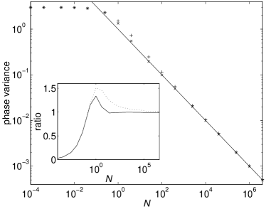
Figure 6: The phase variance as a function of $N$. The numerical results for adaptive and nonadaptive measurements are shown as the crosses and pluses, respectively, and the theoretical values are shown as the continuous line. The inset shows the phase variance as a ratio to the theoretical value of $1/\sqrt{N}$. The results for adaptive and nonadaptive measurements are shown as the continuous line and dotted line, respectively.

These results show that there will be a significant improvement in using an adaptive scheme over a nonadaptive scheme only if the time scale for the system phase variation is comparable to the time between detections. This can be expected from the results for the single-shot case with all photons in one port, where there was a significant improvement in using an adaptive scheme only if the photon number was small. The maximum improvement here is about 24% for $N\approx 4$.

X Conclusions

This study considered the problem of cw phase measurements, where the phase is being varied randomly in time and the aim is to follow this variation with the minimum possible excess uncertainty. We considered three different situations: dyne measurements on a coherent beam, dyne measurements on a (broadband) squeezed beam, and interferometric measurements using a coherent beam input. The relevant dimensionless parameter is $N$, the number of photons per coherence time (the characteristic time for the phase diffusion). Under optimum conditions, we found the analytical results, confirmed numerically, shown in Table 1. Previous results obtained for single-shot measurements on a pulse containing $n$, or $\bar{n}$ on average, photons are also shown for comparison.

Table 1: Scaling of phase variances for large photon numbers $N$ under various measurement conditions. For the cw (continuous-wave) cases, $N$ is the number of photons per coherence time. In the pulsed cases, $n$ ($\bar{n}$) is the (mean) photon number per pulse. Dyne measurements are those performed on a phase-shifted beam or pulse using a local oscillator, while MZI measurements are of a phase shift in one arm of a Mach-Zehnder interferometer. The two empty cells are those not treated in this study, and the question mark denotes a conjectured scaling.

	Coherent, dyne	Squeezed, dyne	Coherent, MZI	Optimal, MZI
cw, adaptive	$N^{-1/2}/2$	$O(N^{-2/3})$	$N^{-1/2}$
cw, nonadaptive	$N^{-1/2}/\sqrt{2}$	$N^{-1/2}\times 3^{1/4}/2$	$N^{-1/2}$
Pulsed, adaptive	$\overline{n}^{-1}/4$	$O(\ln\overline{n}/\overline{n}^{2})$	$n^{-1}$	$O(\ln n/n^{2})?$
Pulsed, nonadaptive	$\overline{n}^{-1}/2$	$\overline{n}^{-1}/4$	$n^{-1}$	$O(n^{-1})$

A number of regularities are evident from this table. With coherent light, the variance reduction offered by adaptive measurements is at most a multiplying factor. With nonclassical light, nonadaptive measurements scale in the same way as for coherent light, but adaptive measurements offer an improvement in the scaling. In all cases, the variance reduction (by a change in the prefactor or the scaling) is less in the cw case than in the pulsed case. This is because in order to obtain the best phase estimate, as $N$ increases, the memory time for the estimate is reduced. This is needed to keep the contribution to the variance from the varying system phase (which increases with memory time) comparable with that from the quantum uncertainty (which decreases with memory time). This means that the effective number of photons used for the estimate is the number per memory time, rather than the number per coherence time, $N$.

In the case of dyne measurements on a coherent beam, it was found that good results were obtained using a simple feedback phase ($\arg A_{t}$), similarly to mark II single-shot measurements semiclass . In the cw case, the feedback simplifies to a form even simpler than for the single-shot case. Specifically, the feedback phase is simply adjusted proportional to the photocurrent. When the correct proportionality constant is selected, a minimum equilibrium phase variance is found that scales as $N^{-1/2}/2$. This is only $\sqrt{2}$ times smaller than the phase variance for heterodyne measurements.

For the case of dyne measurements on broadband squeezed states, the situation is considerably more complicated. The change in the phase cannot be taken to be proportional to the current, but rather is a functional with two parameters. With the degree of squeezing to be optimized as well, there are three parameters that must be varied to find the minimum phase variance. Nevertheless, it is still possible to obtain an analytic result that agrees with the numerical results in its scaling (although predicts the wrong multiplying factor). Specifically, it was found that the minimum phase variance varies as $N^{-2/3}$, compared to $N^{-1/2}$ for a coherent beam. This contrasts with heterodyne measurements on broadband squeezed states, for which the minimum variance is only about 7% below the corresponding result for a coherent beam.

The case for interferometry is more difficult to treat, as it does not work with any simple feedback scheme. The feedback used was based on minimizing the expected variance after the next detection, similarly to the single-shot case. Despite this, it was found that it is possible to determine an approximate theory that agrees reasonably well with the numerical results for the case where a coherent beam enters one port of the interferometer. Similarly to the dyne case with a coherent state, the phase variance is proportional to $N^{-1/2}$. When a linearly changing feedback phase was used (analogous to the heterodyne scheme), it was found that the phase variance is above that for the adaptive feedback, but the difference is very small except for $N$ of order unity. This is as can be expected, as the difference is also very small for large photon numbers in the single-shot case.

In comparison with our previous pulsed results, the cw results obtained in this paper are probably more relevant to, and in some cases easier to implement in, a quantum-optics laboratory. This augurs well for future experimental verification.

References

- (1) H. M. Wiseman, Phys. Rev. Lett. 75, 4587 (1995).
- (2) H. M. Wiseman and R. B. Killip, Phys. Rev. A 56, 944 (1997).
- (3) H. M. Wiseman and R. B. Killip, Phys. Rev. A 57, 2169 (1998).
- (4) D. W. Berry and H. M. Wiseman, Phys. Rev. A 63, 013813 (2001).
- (5) D. W. Berry and H. M. Wiseman, Phys. Rev. Lett. 85, 5098 (2000).
- (6) D. W. Berry, H. M. Wiseman, and J. K. Breslin, Phys. Rev. A 63, 053804 (2001).
- (7) The only case where the feedback phase is not based on this (for dyne measurements) is for the corrections to the close-to-optimal measurements considered in Ref. unpub .
- (8) A. S. Holevo, Lect. Notes Math. 1055, 153 (1984).
- (9) C. W. Gardiner, Quantum Noise (Springer-Verlag, Berlin, 1991).
- (10) D. W. Berry, Ph.D. thesis, The University of Queensland, 2001.
- (11) M. J. Collett, Phys. Scr. T48, 124 (1993).