Squeezed states and quantum chaos

Abstract

We examine the dynamics of a wave packet that initially corresponds to a coherent state in the model of quantum kicked rotator. This main model of quantum chaos, which allows for a transition from regular to to chaotic behavior in the classical limit, may be realized in experiments with cold atoms. We study the generation of squeezed states in the quasiclassical limit and in a time interval when quantum-classical correspondence is yet well-defined. We find that the degree of squeezing depends on the degree of local instability in the system and increases with the Chirikov parameter of stochasticity. We discuss the dependence of the degree of squeezing on the initial width of the packet, the problems of stability and observability of squeezed states at the transition to quantum chaos, as well as the dynamics of wave packet destruction.

I Introduction

At present the problem of squeezed quantum states generation draws a lot of attention, both from the standpoints of pure knowledge and possible applications reviews ; reynaud ; fabre . Most often the topic is squeezed states of the electromagnetic field. If in the simplest case we consider a single-mode quantum field, which is described by the creation $a^{{\dagger}}$ and annihilation $a$ operators, the variances of quadrature field operators $a_{1}=a+a^{\dagger}$ and $a_{2}=-i(a-a^{\dagger})$ satisfy the uncertainty relation $\Delta a_{1}\Delta a_{2}\geq 1$, where the equality holds for a coherent state or vacuum. Then, in these simple terms, a squeezed state is a state for which the variance of one of the quadrature components is less than unity. Quantum fluctuations, determined by the uncertainty relation, can be represented diagrammatically in the $a_{1}-a_{2}$ plane by a circle for a coherent state or by an ellipse for a squeezed state. In a more systematic description of squeezing, the quantum-noise ellipse is determined in terms of the projection onto the $a_{1}-a_{2}$ plane of the horizontal section of the Wigner distribution function, which gives the quasiprobability distribution for measuring the quadrature field components fabre .

A typical situation in experiments on generation of squeezed states is one in which a large number of photons participate in a nonlinear interaction and the amplitude of quantum fluctuations is small compared to the averaged values of the observables reynaud ; fabre . In this case the common approach in explanation of squeezing is to use the semiclassical setting, where the Wigner quantum function is actually replaced by a classical distribution function and instead of examining the dynamics of the quantum-noise ellipse one considers the evolution of the classical phase volume fabre ; heidmann85 .

For quite a long time it has been known that squeezing is enhanced if a system is close to a bifurcation point between two different dynamical regimes fabre ; heidmann85 ; lugiato ; heidmann85a . The increase of squeezing in such conditions was considered, e.g., for the parametric interaction of light waves lugiato and for the interaction of Rydberg atoms with an electromagnetic mode in a high-$Q$ cavity in a dynamical regime close to the separatrix heidmann85 ; heidmann85a . The following simple argument is used to explain the increase of squeezing near a bifurcation point. Quantum fluctuations build up for the physical variable that is unstable near the threshold. As a result there is nothing to stop the strong squeezing for the conjugate variable because of conservation of a phase volume in a nondissipative system fabre .

It must be noted at this point that a number of researchers (see Refs. fabre ; heidmann85 ; lugiato ; heidmann85a ) studied the increase of squeezing near the instability threshold in different optical systems with regular dynamics. However, it is well known that strong (exponential) deformation of the phase volume is one of the main manifestations of dynamical chaos in classical systems sagdeev-book . The physical reason for such strong deformations of the phase volume is the local instability of chaotic motion, which usually manifests itself within a wide range of values of the control parameter of dynamical system. According to the correspondence principle, in the quasiclassical limit a quantum system must mimic the properties of a classical system. Thus, it is quite natural to expect the increase of squeezing at the transition to quantum chaos. On the other hand, in a quantum mechanical description we speak only of the dynamics of wave packets, whose center moves almost along a classical trajectory in the course of a certain time interval. Hence, the strong deformations of the phase volume, which accompany the transition to chaos, must manifest themselves in squeezing along a certain directions in phase space.

As far as we know, the generation of squeezed states in systems with chaotic dynamics was first examined in Refs. alekseev-preprint ; alekseev95 ; chirikov-conf . By employing the $1/N$-expansion method heidmann85a ; yaffe (here $N$ is the number of quantum states participating in the dynamics of the system) it was found in Refs. alekseev-preprint ; alekseev95 that the squeezing of light increases significantly at the transition to chaos during the time interval for which quantum-classical correspondence is well-defined berman-berry . This result was first obtained in Refs. alekseev-preprint ; alekseev95 for the generalized $N$-atoms Janes-Cummings model, which allows a transition from regular to chaotic dynamics in the limit $N\rightarrow\infty$ alekseev88-94 . Later the increase of squeezing at transition to chaos was found for arbitrary single mode quantum optical systems alekseev97-98 . The squeezing of wave packets in conditions of quantum chaos was also briefly discussed in chirikov-conf . However, the main results of works alekseev-preprint ; alekseev95 ; alekseev97-98 were obtained by using a form of perturbation theory (the $1/N$-expansion). Therefore it is important to investigate the generation of squeezed states at transition to quantum chaos in a simple quantum system whose time evolution can be found explicitly.

In the present paper we study the generation of squeezed states in the time evolution of an initially Gaussian wave packet in the model of quantum kicked rotator. This model was first introduced by Casati et al. casati79 and at present is the main model in studies of quantum chaos (for review see chirikov81 ; 15 ; casati95 ). The quantum rotator model is attractive mainly for two reasons: (i) the classical limit for this model is a well-known standard map chirikov79 , and (ii) it is fairly easy to study numerically the dynamics of the model for a large number of quantum levels.

We examine the dynamics of narrow Gaussian packets in a rotator with $2^{17}(\simeq 10^{5})$ levels. We define squeezing for the generalized quadrature operator $X_{\theta}=a\exp(-i\theta)+a^{\dagger}\exp(\theta)$, where $\theta$ is a real parameter. It is just $X_{\theta}$ that is observed in the homodyne detecting scheme, where $\theta$ is determined by the phase of the reference beam reviews . We will see that as long as the wave packet is localized, the degree of squeezing correlates well with the degree of local instability in the system. Here the greater the instability, the stronger the squeezing achieved in a shorter time interval. Squeezing is much stronger for quantum chaos than it is for regular motion. We will also see that the narrower the initial wave packet, the higher the degree of squeezing that can be achieved. We attribute this to the fact that a narrow wave packet is closer in its time evolution to the classical trajectory than a broad one, with the result that it is more sensitive to local instabilities in the motion, which leads to stronger squeezing.

We will also consider the problem of stability and observability of squeezed states in the transition to chaos. More precisely, we will study the time dependence of the optimum values of the phase $\theta$ of the generalized quadrature operator $X_{\theta}$ for which the squeezing is maximal (so-called principal squeezing luks ; tanas ). We will show that in conditions of strong chaos and for long enough time, the optimum values of the phases change dramatically even under a small perturbation of the parameters of the initial Gaussian wave packet. Such a squeezing regime is unstable and difficult to observe. On the other hand, our results suggest that for weak chaos squeezing is fairly stable.

We will also briefly discuss the dynamics of disintegration of wave packets at chaos. Here we will show that a typical scenario of disintegration of an initially localized wave packet in chaos consists of two stages: the initial spread of the wave packet, and the catastrophic disintegration of the packet into many small subpackets. Here our results agree on the whole with the results of Casati and Chirikov casati95 .

Note that earlier the dynamics of narrow Gaussian wave packets in the quasiclassical limit was studied numerically for the models of a quantum kicked rotator fox1 ; lan , quantum kicked top fox2 , and quantum Arnold cat elston-preprint in connection with the problem of quantum-classical correspondence at quantum chaos. However, in these papers the generation of squeezed states was not considered.

The model of a quantum kicked rotator is very popular in theoretical studies of quantum chaos. On the other hand, recently possibilities of implementing variants of this model in optical systems have been discussed stand-opt-exp . Moreover, the model of quantum rotator has been realized in experiments on the interaction of laser beam and cooled atoms atom-opt-exp . Hence our results on the increase of squeezing at the transition to quantum chaos in a kicked quantum rotator are also directly related to experimentally realizable systems.

The plan of the paper is as follows. In Sec. II we discuss the quantum standard map and find how to calculate principal squeezing. The method used in numerical simulations is developed in Sec. III, and the main results on the dynamics of squeezing are given in Sec. IV. Finally, in Sec. V we draw the main conclusions and consider the possibility of verifying our results in experiments.

II The model of quantum kicked rotator and squeezed states

Consider the model of a quantum rotator with periodic delta-kicks. Here we follow the notation of Ref. lan . The Hamiltonian is

$$H = \frac{p^{2}}{2mL^{2}}-\delta_{p}(t/T)mL^{2}\omega_{0}^{2}\cos{(x)},$$

$$\delta_{p}(t/T)=\sum_{j=-\infty}^{+\infty}\delta(j-t/T),$$

where $x$ is the cyclic variable with a period $2\pi$, $L$ is the characteristic size of the rotator, $m$ is the rotator mass, and $\omega_{0}$ is the frequency of linear oscillations. The function $\delta_{p}(t/T)$ describes a periodic sequence of kicks with a period $T$, where $\delta(x)$ is the Dirac $\delta$-function. Let us introduce new variables

$$\alpha=mL^{2}\omega_{0}^{2}T,\quad\beta=\frac{T}{mL^{2}}$$ (2)

and measure time in units of $T$, i.e., $t\to t/T$. Then the Schrödinger equation takes the form

$$i\hbar\frac{\partial\Psi}{\partial t}=-\frac{\hbar^{2}\beta}{2}\frac{\partial^{2}\Psi}{\partial x^{2}}-\delta_{p}(t)\alpha\cos{(x)}\Psi.$$ (3)

Due to the periodicity of $\Psi(x)$ in $x$ the solution of Eq. (3) can be written as follows

$$\Psi(x) = \frac{1}{\sqrt{2\pi}}\sum_{k=-\infty}^{+\infty}e^{ikx}A_{k}(t),$$

$$A_{k}(t) = \frac{1}{\sqrt{2\pi}}\int_{0}^{2\pi}\Psi(x)e^{-ikx}dx.$$ (4)

Using the standard procedure chirikov81 ; lan , we obtain the quantum map in the form

$$\Psi_{n+1} = U_{x}U_{p}\Psi_{n},$$

$$U_{p}=\exp{\left(-\frac{i\beta}{2\hbar}\hat{p}^{2}\right)},\quad U_{x}=\exp{\left(\frac{i\alpha}{\hbar}\cos{(\hat{x})}\right)},$$

where $\Psi_{n}$ is the value of the wave function at the time moment immediately after the $n$-th kick. The time evolution of the wave function in the map (II) is determined solely by two parameters, $\alpha/\hbar$ and $\beta\hbar$. Since $U_{p}$ is diagonalized in the $p$-representation, $U_{x}$ is diagonalized in the $x$-representation, and the transition between $x-$ and $p$-representations is given by the Fourier transformation (II), the map (II) actually reduces to

$$\Psi_{n+1}(x)=U_{x}F^{-1}U_{p}F\Psi_{n}(x),$$ (6)

where $F$ and $F^{-1}$ are the direct and inverse Fourier transforms.

Sometimes it proves useful to use the quantum map written in terms of the probability amplitudes $A_{k}$ of transitions between the unperturbed levels of the rotator casati79 . Combining Eqs. (II) and (II), we obtain

$$A_{k}^{(n+1)} = \sum_{m=-\infty}^{+\infty}F_{km}A_{m}^{(n)},$$

$$F_{km}=(-i)^{k-m}\exp{\left(-\frac{i\hbar\beta m^{2}}{2}\right)}J_{k-m}\left(\frac{\alpha}{\hbar}\right),$$

where $J_{l}(z)$ is the Bessel function of order $l$ and argument $z$, and the superscript $(n)$ on the variable $A$ stands for the number of the kick. Bearing in mind that the Bessel functions with $\mid l\mid\geq z$ rapidly decrease with increasing $l$, we see from Eq. (II) that, with exponential accuracy, in the course of a single kick $2\alpha{\hbar}^{-1}$ unperturbed rotator levels are captured. Below we consider the case where $\alpha/\hbar$ is large, which is typical of quantum chaos problems.

In the classical limit the Hamiltonian (II) reduces to the standard map

$$P_{n+1}=P_{n}-K\sin x_{n+1},\quad x_{n+1}=x_{n}+P_{n}\pmod{2\pi},$$ (8)

where $P_{n}=\beta p_{n}$, the subscript $n$ denoting the values of $x$ and $P$ immediately after the $n$-th kick, and $K\equiv\alpha\beta$ is the Chirikov parameter. Strong and global chaos sets in for $K>1$. For $K<1$ the larger part of the phase plane is filled with regular trajectories, although small regions with local chaos exist no matter how small $K$ may be chirikov79 . The phase portrait for the map (8) at $K=0.8$ is depicted in Fig. 1. The chaotic layer lies near the separatrix of the main resonance, which passes through the hyperbolic points $(\pm\pi,0)$. In our calculations we usually take a wave packet whose center is located near a hyperbolic point but yet in a region of regular motion at $K<1$.

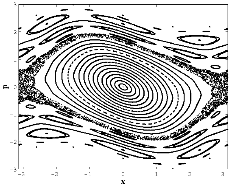
Figure 1: Phase portrait of the classical standard map for $K=0.8$.

For the initial state of the quantum map (II) we take the Gaussian wave packet

$$\Psi(x)=(2\pi\sigma^{2})^{-1/4}\exp{\left(-\frac{(x-x_{0})^{2}}{4\sigma^{2}}+ik_{0}(x-x_{0})\right)},$$ (9)

where $\langle x\rangle=x_{0}$, $\langle\delta x^{2}\rangle\equiv\langle x^{2}\rangle-\langle x\rangle^{2}=\sigma^{2}$, $p_{0}\equiv\langle p\rangle=\hbar k_{0}$, $\langle\delta p^{2}\rangle=\frac{\hbar^{2}}{4\sigma^{2}}$ and $k_{0}$ is an integer. The packet is assumed narrow: $\sigma\ll x_{0}$ and $\langle\delta p^{2}\rangle\ll\hbar k_{0}$. Note that in view of its periodicity in $x$ the wave packet (9) is generally not a state that minimizes the uncertainty relation. But in the case of a narrow packet it is essentially indistinguishable from a minimum-uncertainty state fox1 ; lan ; fox2 .

A typical initial quantum state in studies of light squeezing is a coherent state reviews ; reynaud ; fabre . Such a state is an eigenfunction of the annihilation operator $a$, which in the present notation can be written as

$$a=\frac{1}{\sqrt{2\hbar}}(\sqrt{\gamma}\hat{x}+i\frac{\hat{p}}{\sqrt{\gamma}}),\quad\gamma={\left(\frac{\alpha}{\beta}\right)}^{1/2}.$$ (10)

The fact that the annihilation operator has such an appearance can easily be understood if we consider the following limiting case of the harmonic oscillator that follows from (3):

$$i\hbar\frac{\partial\Psi}{\partial t}=-\frac{\hbar^{2}\beta}{2}\frac{\partial^{2}\Psi}{\partial x^{2}}+\frac{\alpha x^{2}}{2}\Psi.$$ (11)

Now we can show that the wave function (9) is a coherent state, i.e., an eigenfunction of operator (10), if we put

$$\sigma^{2}=\frac{\hbar}{2\gamma}.$$ (12)

Let us now turn to the problem of squeezing. In light squeezing experiments reviews , the observable quantity is the variance of the generalized quadrature operator

$$X_{\theta}=ae^{-i\theta}+a^{\dagger}e^{i\theta},$$ (13)

where $\theta$ is the phase of the reference beam in the homodyne detecting scheme. In the particular cases where $\theta=0$ and $\theta=\pi/2$, Eq. (13) yields the following expressions for the generalized position and momentum operators

$$X_{1}=a+a^{\dagger},\quad X_{2}=-i(a-a^{\dagger}),\quad[X_{1},X_{2}]=2i$$ (14)

with the uncertainty relation $\langle\delta X_{1}^{2}\rangle\langle\delta X_{2}^{2}\rangle\geq 1$, where averaging is done over an arbitrary quantum state and equality is achieved for a coherent state. The standard definition of quadrature squeezing is the condition reviews ; fabre

$$\min{\left(\langle\delta X_{1}^{2}\rangle,\langle\delta X_{2}^{2}\rangle\right)}<1,$$ (15)

i.e., the variance of one of the quadrature components is smaller than for the coherent state.

In a more general case we consider the variance $\langle\delta X_{\theta}^{2}\rangle$ of the operator (13), and the state is assumed squeezed if the value of $\langle\delta X_{\theta}^{2}\rangle$ in this state for some value of $\theta$ is smaller than in the coherent state luks ; tanas . Experiments actually determine the minimum $S$ of this variance as a function of the angle $\theta$ as

$$S=\min_{\theta\in[0,2\pi]}{\langle\delta X_{\theta}^{2}\rangle}.$$ (16)

Using the definition (13) of $X_{\theta}$, it is possible to show luks ; tanas that

$$S=1+2\langle\delta a^{\dagger}\delta a\rangle-2\sqrt{\langle\delta a^{2}\rangle\langle\delta a^{{\dagger}2}\rangle}$$ (17)

and the minimum of $\langle\delta X_{\theta}^{2}\rangle$ is reached at an optimum phase value $\theta=\theta^{*}$ defined as follows tanas :

$$e^{2i\theta^{*}}=-\sqrt{\langle\delta a^{2}\rangle/\langle\delta a^{{\dagger}2}\rangle}$$ (18)

For our discussion it is convenient to express S in terms of the cumulants of the operators $x$ and $p$. Using the definition (10) of operator $a$ and Eq. (17), we obtain

$$S=\frac{1}{\hbar}\left(\frac{\langle\delta p^{2}\rangle}{\gamma}+\langle\delta x^{2}\rangle\gamma-\sqrt{(\langle\delta x^{2}\rangle\gamma-\langle\delta p^{2}\rangle/\gamma)^{2}+4c^{2}}\right),$$ (19)

where $c=\frac{1}{2}(\langle(xp+px)\rangle-2\langle x\rangle\langle p\rangle)$ Clearly for any Gaussian wave packet $S=\frac{\hbar}{2\sigma^{2}\gamma}$, while for a coherent state we have $S=1$ because of equality (12). Hence a state is squeezed if

$$S<1$$ (20)

The condition determines the principal squeezing attainable in homodyne detection luks . The maximum of the variance $\langle\delta X_{\theta}^{2}\rangle$ in $\theta$ can be defined in the same way the minimum was defined in Eq. (16). We denote it by $\overline{S}$. Then we can show that the dependence of $\overline{S}$ on the cumulants differs from Eq. (19) only in the sign in front of the square root, so that we have

$$S\overline{S}\geq 1.$$ (21)

Thus, squeezing in $S$ (Eq. 20) is accompanied by dilation in $\overline{S}$. Note that in contrast to the quadrature squeezing (15), the definition of principal squeezing (19) contains quadrature correlators of the $\langle xp\rangle$ type. This is very important for systems with discrete time, to which the model of a quantum kicked rotator belongs. The thing is that the quadrature squeezing (15) is essentially unobservable in such systems, although the principal squeezing (19) and (20) may occur . We will discuss the time dependence of $S$ in Sec. IV.

III The numerical method

Several features of the numerical method must be mentioned. The interval in $x$ from $0$ to $2\pi$ is partitioned into $N$ segments $\triangle x=2\pi/N$, and the wave function $\Psi(x)$ is represented by a discrete sequence of values (column vector $\mid\Psi\rangle$) of length $N$, so that $\Psi_{l}=\Psi(l\triangle x)$, $l\in[0,1,\ldots,N-1]$. Accordingly, $k$ varies from $0$ to $N-1$ in the sum (II). In our numerical method $N$ is always an integral power of two and the operator $F$ in Eq. (6) is represented in the form of the fast Fourier transform inducing the transformations

$$F:\Psi_{l}\to A_{k},\quad F^{-1}:A_{k}\to\Psi_{l}$$ (22)

To determine the principal squeezing, we must calculate $\langle\delta q^{2}\rangle$, $\langle\delta p^{2}\rangle$, and $\langle xp\rangle$ (see Eq. (19)). For instance, the calculation of $\langle xp\rangle$ proceeds along the following lines

$$\langle xp\rangle=\langle\Psi|\vec{x}F^{-1}\vec{p}F|\Psi\rangle,$$

where $\langle\Psi|$ is obtained by transposing the vector $|\Psi\rangle$ and then finding the complex conjugate of the result, while $\vec{x}$ and $\vec{p}$ are vectors that initially have the form $\vec{x}=[0,\triangle x,2\triangle x,\ldots,2\pi-\triangle x]$, $\vec{p}=[0,1,2,\ldots,N-1]$.

The fact that $x$ is defined in $\pmod{2\pi}$ requires following the wave packet and ensuring that it is defined correctly during the passage through the end-points of the interval $[0,2\pi]$. We set up the process in the following manner. When the center of the wave packet in the $x$-representation approaches an edge of the half-interval $[0,2\pi[$, the wave function $\Psi(x)$ is examined on a new interval, $[-\pi,\pi[$, with a new vector $\vec{x}=[0,\triangle x,\ldots,\pi,-\pi+\triangle x,-\pi+2\triangle x,\ldots,-2\triangle x,-\triangle x]$, since $(-k\triangle x)\bmod{2\pi}=(2\pi-k\triangle x)\bmod{2\pi}$, where $k$ is an integer. The transition from $[-\pi,\pi[$ to $[0,2\pi[$ is treated similarly.

Calculations in the $p$-representation have their own special features. Although for the Hamiltonian (II) the momentum is defined in the interval from $-\infty$ to $+\infty$, in numerical calculations we deal only with a finite range of values of momentum $p$, which is specified by the number terms $N$ in the Fourier transform (II). To avoid the possible problem of reflection of the wave packet from an edge of the given interval in the $p$-representation, we select this interval in each iteration of map (6) in such a way that the maximum of the absolute value of the wave function of the packet is always at the center of the given interval (actually, we renumber the vector $\vec{p}$).

The process of calculating the next iteration of the quantum map (6) is terminated as soon as the wave packet ceases to be sufficiently localized either in the $x$-representation or in the $p$-representation, i.e., when the number of terms in the Fourier transformation actually involved in the calculation process is smaller than needed. Let us now to present the conditions for wave packet delocalization, which we use in our numerical simulations. First, introduce the notations $\xi=\max_{[0,2\pi]}|\Psi(x)|$, $\chi=\max\{|A_{1}|,|A_{2}|,\ldots,|A_{N}|\}$. Next, introduce $A_{left}$ ($A_{right}$), the values of $A_{k}$ belonging, respectively, to the left and right edges of the finite interval in which the wave function in momentum space is determined. The wave packet is delocalized and further calculations are terminated when one of the two inequalities,

$$\max\{|A_{left}|/\chi,|A_{right}|/\chi\}>\varepsilon\quad\mbox{or}\quad|\Psi(z)|/\xi>\varepsilon$$

become valid (here $z=0$, if $x\in[0,2\pi[$ or $z=\pi$ if $x\in[-\pi,\pi[$). In this paper we used the cut off value $\varepsilon=0.002$.

IV The main results

As an initial wave function in our calculations we took the coherent state (a Gaussian wave packet) with $\hbar=10^{-6}$, $k_{0}=10000$, and $\sigma$ was varied between 0.04 and 0.07. We fixed the initial width of the wave packet $\sigma$ and the value of Chirikov parameter $K$. Then, the parameters $\alpha$ and $\beta$ in the evolution operator (II) are

$$\alpha=K^{1/2}\frac{\hbar}{2\sigma^{2}},\quad\beta=K^{1/2}\frac{2\sigma^{2}}{\hbar}.$$ (23)

These formulas are obtained by combining the definition $K=\alpha\beta$ and Eqs. (10) and (12). In Sec. II we found that the number of unperturbed levels of rotator captured in one kick is $\approx 2\alpha/\hbar$. From (23) it follows that in our case this number is $K^{1/2}/\sigma^{2}$ and amounts to several tens of thousands for the adopted widths of the wave packet.

In our calculations $K$ was varied between 0.2 and 2 with a step of 0.02. We found the time dependence of the squeezing $S$ (19) and the optimum value of the phase $\theta^{*}$ at which $\langle\delta X_{\theta}^{2}\rangle$ is at its minimum. To demonstrate the correlation that exists between the degree of squeezing and characteristics of chaos alekseev95 ; alekseev97-98 we calculated

$$d=[\langle\delta x^{2}\rangle+\langle\delta p^{2}\rangle]^{1/2}.$$ (24)

It can be shown alekseev95 ; alekseev97-98 ; sundaram that in the classical limit and while the wave packet is well-localized, i.e., $[\langle\delta x^{2}\rangle]^{1/2}\ll x_{0}$ and $[\langle\delta p^{2}\rangle]^{1/2}\ll p_{0}$, the $d$ of (24) corresponds to the following distance in phase space

$$d_{cl}(t)=[(\Delta x)^{2}+(\Delta p)^{2}]^{1/2},$$ (25)

where $\left(\Delta x(t),\Delta p(t)\right)$ is the solution of the linear small-perturbation equations near the classical trajectory $\left(x(t),p(t)\right)$. The quantity $d_{cl}(t)$ characterizes the divergence of two initially close trajectories and enters into the definition of the largest classical Lyapunov exponent

$$\lambda=\lim_{t\rightarrow\infty}\frac{d_{cl}(t)}{t}.$$ (26)

For a classical standard map in conditions of strong chaos, $K\gg 1$, there exists the simple dependence $\lambda\approx\ln(K/2)$ chirikov79 . Lyapunov exponent (26) is an asymptotic characteristic of chaos. For finite time intervals sagdeev-book

$$d_{cl}(t)\simeq\exp(h(x,p)t),$$ (27)

where the exponent $h$ is a function of a point in phase space and coincides, in order of magnitude, with the Lyapunov exponent $\lambda$, but in some time intervals the difference between the two may be significant. The latter fact can be explained by the strong inhomogeneity in the statistical properties of the phase space of chaotic systems and, correspondingly, by the different rates of divergence of trajectories in different regions of phase space through which the system passes in its time evolution. It must be noted at this point that the dependence of $h$ on the parameter $K$ is rather complicated. What is important, however, is only the property of the strong (exponential) increase of $d_{cl}$ (27) in the presence of chaos, a property often called local instability sagdeev-book . When the motion is regular, the time dependence of $d_{cl}$ is much weaker – it follows a power function sagdeev-book .

On the other hand, it is $h$ that determines the rate of phase volume deformation: the stronger the local instability, the greater the deformation of phase volume in a given time interval. Since in our case quantum-classical correspondence and the concept of chaos are well-defined only in a very short time interval, while the wave packet remains localized, it is meaningful to consider the correlations existing between the time dependence of the squeezing and that of the quantity $d$ (see (24)), which in the classical limit becomes $d_{cl}$ (see (25)).

Figure 2 depicts the time dependence of the logarithm of squeezing $\ln S$ and $\ln d$ for different values of $K$, when the

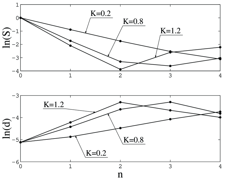
Figure 2: Upper part of the figure: Time dependence of the logarithm of squeezing $\ln S$. Lower half of the figure: Time dependence of $\ln d$ (see Eq. (24)). Everywhere $x_{0}=\pi$ and $\sigma=0.006$.

center of the wave packet is initially located at the point $x_{0}=\pi$, $p_{0}=\hbar k_{0}=0.01$. This initial condition is close to a hyperbolic point through which the chaotic layer passes even when $K$ is small (see Fig. 1). Figure 2 shows that the larger the squeezing (the smaller the value of $S$) the larger the local instability (the larger the values of $\ln d$). This valid up to $n\approx 4$, when the packet spread becomes so large that purely quantum effects become important.

For another initial condition, $x_{0}=\pi/2$, $p_{0}=0.01$, which is closer to an elliptic point and hence lands in the chaotic region only at large values of $K$, the dynamics of squeezing is depicted in Fig. 3.

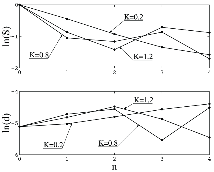
Figure 3: Same as in Fig. 2 but for $x_{0}=\pi/2$.

We see that in this case squeezing is in about two orders stronger than in the conditions of Fig. 3 in the same time interval. On the other hand, both Fig. 2 and Fig. 3 exhibit an increase of squeezing as a function of the parameter $K$, which controls the strength of chaos in the system.

Now we turn to study of the correlation between squeezing and the degree of local instability at different $K$ in greater detail. The $K$-dependence of the degree of squeezing calculated after a fixed number of kicks at $x_{0}=\pi$ and $p_{0}=0.01$ is depicted in Fig. 4.

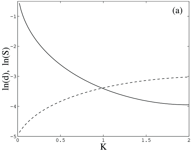
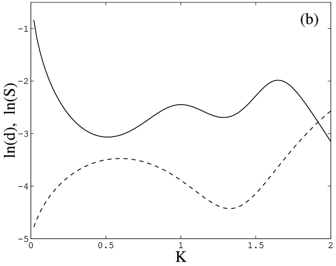
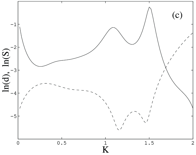
Figure 4: The dependencies of $\ln S$ (solid curves) and $\ln d$ (dashed curves) on the Chirikov parameter $K$ at a fixed number of kicks: (a) $n=3$, (b) $n=4$, (c) $n=5$. Everywhere $x_{0}=\pi$ and $\sigma=0.007$.

After the third kick the correlation between $\ln S$ and $\ln d$ become very evident (Fig. 4a). However, small discrepancies in this dependence may appear as the number of kicks grows. Such discrepancies become evident, for instance, after the fourth kick for $1.1\lesssim K\lesssim 1.4$ (Fig. 4b). After five kicks, $n=5$, the correlation between $\ln S$ and $\ln d$ is restored (Fig. 4c). Note that this behavior pattern is quite typical. Hence, to establish the correlation between local instability and squeezing more clearly, a certain procedure of coarsening (averaging) these quantities in the given time interval is needed. In our study we determine the minimal squeezing, $S_{min}$, and the maximal $d_{max}$ in a time interval during which the packet remains well localized for most values of $K$ considered here. We found that there is a distinct correlation between $S_{min}$ and $d_{max}$: the larger the value of $d_{max}$ the smaller the value of $S_{min}$, and vice versa. An example of such a dependence is depicted in Fig. 5, where $S_{min}$ and $d_{max}$ were calculated after six kicks.

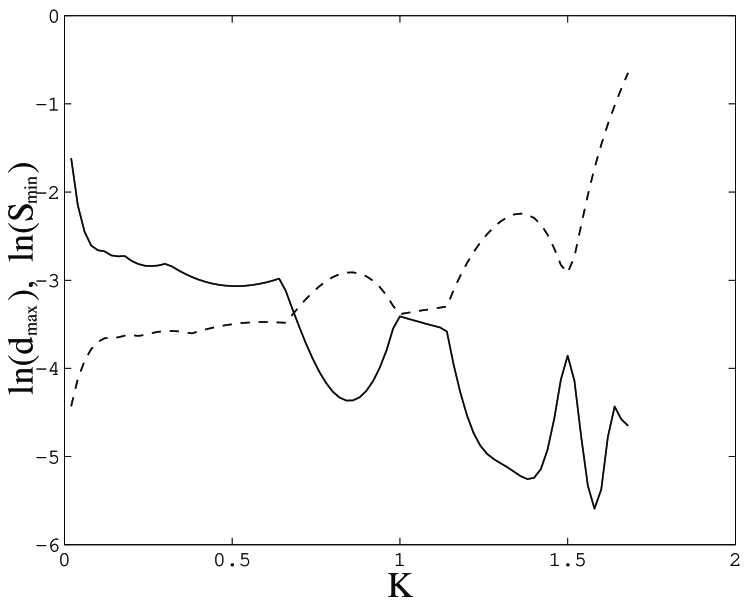
Figure 5: Logarithm of the minimal squeezing $S_{min}$ (solid curve) and logarithm of the maximal local instability $d_{max}$ (dashed curve) as functions of the Chirikov parameter $K$ after seven kicks. Other parameters and initial conditions are the same as in Fig. 4.

Note that the diagrams do not go farther than $K>1.7$ because after six kicks the wave packet becomes delocalized for $K>1.7$ and calculating averages and local instability becomes meaningless.

We also studied the dependence of the dynamics of squeezing on the initial width of the wave packet $\sigma$. The results are depicted in Fig. 6.

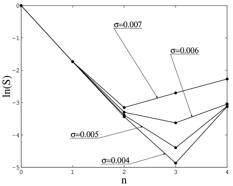
Figure 6: Time dependence of the logarithm of squeezing $S$ for different initial widths of the wave packet $\sigma$ and at fixed values $K=0.8$, $x_{0}=\pi$.

Clearly, the narrower the packet the stronger the squeezing achieved in a fixed time interval. This dependence arises because a narrow wave packet travels farther along its classical trajectory than a wide packet, so that it undergoes stronger deformations related to nonlinear classical dynamics. The exponential decrease is replaced by growth when the wave packet departs from the classical limit and the dynamics is of an essentially quantum nature.

Now examine the problem of stability and observability of squeezing in conditions of chaos. The figures mentioned earlier can serve to illustrate the statement that the stronger the chaos the stronger the principal squeezing. However, the definition of principal squeezing (19) is related to fixing the phase, $\theta=\theta^{*}$. Here $\theta^{*}$ is time dependent even for exactly integrable systems tanas . For strong chaos in the classical limit, the time dependence of $\theta^{*}$ may be very complicated. Indeed, in addition to stretching and squeezing, the main feature of classical chaos in the systems with bounded phase space is the multiple formation of folds of the phase volume as a system evolves sagdeev-book . Hence the process of finding the “minimum width” of a phase drop, which actually amounts to finding the dependence $\theta^{*}$ vs $t$ in the quasiclassical limit, becomes unstable for large time intervals.

Basing our reasoning on a similar semiclassical picture, we examined the stability of the time dependence of the optimal phase $\theta^{*}(t)$, which was calculated quantum mechanically, against a small perturbation of the initial position of the wave packet. More precisely, we found the time dependence of the optimal phase $\theta_{1}^{*}$ with the initial condition $x_{0}=\pi$ and, similarly, $\theta_{2}^{*}(t)$ with the initial condition $x_{0}=\pi-0.05$. We denote the difference of these phases by

$$D(t)=\theta_{1}^{*}(t)-\theta_{2}^{*}(t).$$ (28)

Since $\theta^{*}(t)$ is periodic with a period $\pi$ (see Eq. (18), it is natural to take $\sin(2D)$ as the quantity of interest, since m this way we avoid breaks in the diagrams related to the periodicity of $\theta^{*}(t)$. The dependence of $\sin(2D)$ on the Chirikov parameter $K$ for different fixed numbers of kicks is depicted in Figs. 7a-7c.

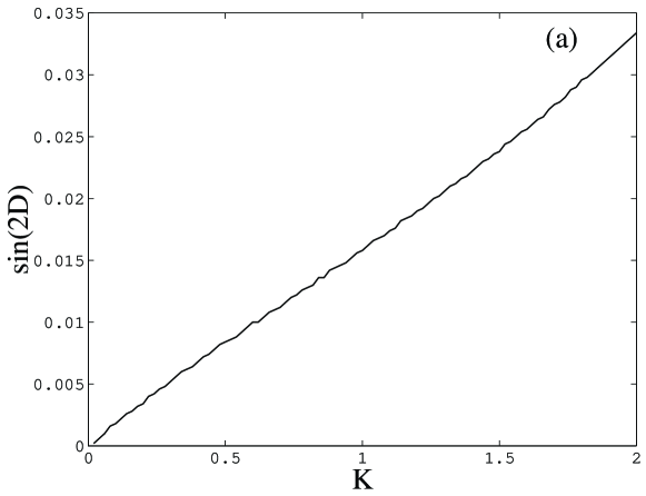
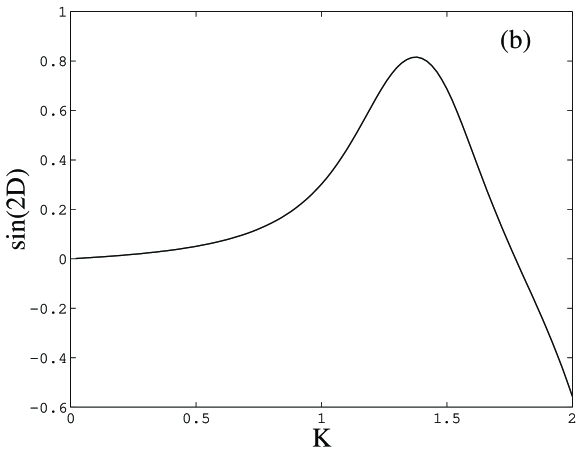
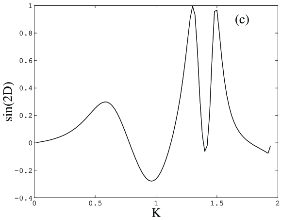
Figure 7: The difference of optimal phases $D$ (see Eq. (28)) as a function of the Chirikov parameter $K$ at a fixed number of kicks: (a) $n=2$, (b) $n=3$, and (c) $n=4$. Everywhere $x_{0}=\pi$ and $\sigma=0.006$.

After two kicks (Fig. 7a) the maximum value of $\mid\sin(2D)\mid$ does not exceed 0.035 at $K=2$. After three kicks ((Fig. 7a) the value of $D$ becomes significant at $K\gtrsim 1.2$. Finally, after four kicks (Fig. 7c) the process of measuring squeezing becomes essentially unstable at $K\gtrsim 1$. Indeed, in these conditions with a small perturbation of the initial position of the wave packet, the difference of the optimum phases reaches a value of order $\pi$. Such regime of squeezed states generation was called unstable squeezing in alekseev95 . As Fig. 7 implies, unstable squeezing is observed when chaos is strong. On the other hand, for short time intervals and small values of $K$, the squeezing can be already strong enough but yet rather stable.

To conclude this section we will briefly touch on the problem of the dynamics of disintegration of coherent states in conditions of chaos, a problem that is of interest by itself. Figures 8a and 8b depict the dependence of $\mid\Psi\mid$ on $x$ and of $\mid A\mid$ on $k$ (see Eq. (II)).

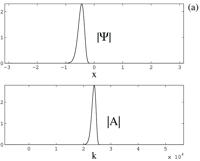
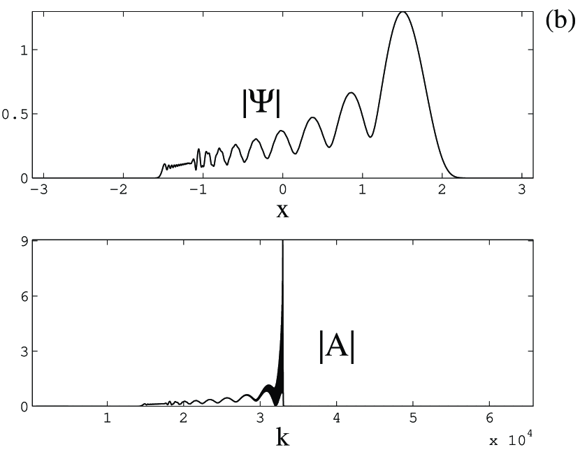
Figure 8: Dependence of absolute value of the wave function $\mid\Psi\mid$ on $x$ and dependence of the absolute value of the Fourier transform $\mid A_{k}\mid$ on $k$ (see Eq. (II)) at (a) $n=6$, (b) $n=18$. Everywhere $K=1.2$, $x_{0}=\pi$ and $\sigma=0.006$.

Actually, Fig. 8 gives the shape of the wave function in the coordinate and momentum representations for an initially narrow wave packet with $[\langle\delta x^{2}\rangle]^{1/2}(t=0)\equiv\sigma=0.006$ and $[\langle\delta p^{2}\rangle]^{1/2}(t=0)=(1/12)\times 10^{-3}$. The relatively small value $K=1.2$ makes it possible to examine the fairly long evolution of the wave packet up to the point of its total disintegration. After six kicks (Fig. 8a) the wave packet spreads out significantly, but on the whole retains its bell shaped structure. What follows is a disintegration of the packet into many small subpackets, with the characteristic shape of the wave function depicted in Fig. 8b (after 18 kicks). Finally, very soon the wave function becomes so dissected that even $2^{17}$ Fourier harmonics are insufficient to describe the evolution correctly (for the data of Fig. 8 this happens approximately at the 20th kick).

Qualitatively, the same pattern of the evolution of the wave packet was observed at higher values of $K$: first the broadening of the wave packet, and then its rapid disintegration into many very small subpackets. The differences in packet disintegration for large values of $K$ in comparison with the case $K\simeq 1$ (as in Fig. 8) boil down to two facts:(i) the “swelling of the packet” and the disintegration occur very rapidly (it takes only several kicks to complete the process), and (ii) the emerging subpackets are extremely small. Hence the process of disintegration of wave packets in strong chaos resembles an explosion. On the whole, the pattern being described agrees well with the pattern obtained from the analysis of the behavior of the Wigner function casati95 , although we observed some anomalies. In particular, for fairly narrow wave packets ($\sigma=4\times 10^{-3}$) we observed the disintegration of the initial packet into two fairly large subpackets. Ripples then appeared on the subpackets, and the two disintegrated into many small packets. A more detailed description of the disintegration of coherent states at chaos will be a subject of our separate publication.

V Discussion and conclusion

Thus, in this work we numerically study the dynamics of generation of squeezed states in the evolution of a Gaussian wave packet in the quasiclassical limit for the model of a kicked quantum rotator. We show that within the time interval where the packet is well-localized the squeezing becomes stronger in the transition to chaos. For strong chaos and in long time intervals, the squeezing process becomes unstable. These results, obtained through direct numerical simulation, are in good agreement with the results derived using perturbation theory for other models alekseev-preprint ; alekseev95 ; alekseev97-98 .

In the final stages of preparing the manuscript for press we became acquainted with two recent papers xie also devoted to the problem of generating nonclassical states (squeezing and antibunching) in the systems with quantum chaos. The authors of Ref. xie presented the results of numerical experiments on the dynamics of quadrature squeezing in simple quantum models that allow a transition to chaos in the classical limit: the Lipkin-Meshkov-Glick model lipkin and the Belobrov- Zaslavsky-Tartakovskil model belobrov . In contrast to our approach, the authors of paper xie were interested in the long-time limit, when the wave packets are delocalized and this sense the quantum-classical correspondence is completely violated. They found that quadrature squeezing disappears at the transition to quantum chaos, although to some degree squeezing is always present in conditions of regular motion. The nonzero squeezing in the conditions of quantum chaos and in short-time limit has been also mentioned in xie , but the enhance of squeezing was not observed, probably because in their numerical simulations the quasiclassical parameter was not large enough: only several hundred of quantum levels participated in the dynamics of the system. Thus, the results of xie do not contradict ours but supplement them in another limiting case, the limit of long times of motion.

In conclusion we would like to make a remark concerning the possibility of observation of squeezing in quantum chaos on a time scale corresponding to a well-defined quantum-classical correspondence. At present essentially all experiments on light squeezing are done in the stationary regime. Squeezing at the transition to quantum chaos increases only over finite time intervals and in this sense is a transient dynamical phenomenon. We hope that the development of effective experimental methods for observing squeezed states of light in transient dynamical regimes will also make it possible to observe the enhanced squeezing at the transition to quantum chaos. On the other hand, as noted in the Introduction, it is much simpler to realized the quantum kicked rotator model in atomic optics atom-opt-exp . Moreover, it is much simpler to observe transient dynamical regimes in experiments with cold atoms. Hence we believe that atomic optical systems have great potential for observations of squeezed states at transition to quantum chaos.

We are grateful to Andrey Kolovsky and Jan Peřina for discussions and to Boris Chinkov for support and drawing our attention to his work chirikov-conf .

References

- (1) Current address: Division of Theoretical Physics, Department of Physical Sciences, Box 3000, University of Oulu FIN-90014, Finland. E-mail: Kirill.Alekseev@oulu.fi
- (2) D. F. Smimov and A. S. Troshin, Usp. Fiz. Nauk 153, 233 (1987) [Sov. Phys. Usp. 30, 851 (1987)]; M. C. Teich and B. E. A. Saleh, Phys. Today 43(6), 26 (1990) [Russ. Transl.: Uspekh. Fiz. Nauk 161, 101 (1991)].
- (3) S. Reynaud, A. Heidmann, E. Giacobino and C. Fabre, in Progress in Optics XXX, edited by E. Wolf, Elsevier, Amsterdam (1992), p. 1.
- (4) C. Fabre, Phys. Rep. 219, 215 (1992).
- (5) A. Heidmann, J. M. Raimond, and S. Reynaud, Phys. Rev. Lett. 54, 326 (1985).
- (6) L. A. Lugiato, P. Galatola, and L. M. Narducci, Opt. Commun. 76, 276 (1990).
- (7) A. Heidmann, J. M. Raimond, S. Reynaud, and N. Zagury, Opt. Commun. 54, 189 (1985).
- (8) R. Z. Sagdeev, D. A. Usilov and G. M. Zaslavsky, Nonlinear Physics: From the Pendulum to Turbulence and Chaos, (Harwood Academic, New York, 1988) [Russian edition: Nauka, Moscow, 1988].
- (9) K. N. Alekseev, “Squeezed states generation in nonlinear system with chaotic dynamics”, Preprint Kirensky Institute of Physics 674F, Krasnoyarsk (1991).
- (10) K. N. Alekseev, Opt. Commun. 116, 468 (1995), see also Eprint quant-ph/9808010 .
- (11) B. V. Chirikov, The uncertainty principle and quantum chaos, in Proc. of 2nd Intern. Workshop on Squeezed States and Uncertainty Relations, Moscow 25-29 May, 1992, NASA Conference Publication 3219, 317 (1993).
- (12) L. G. Yaffe, Rev. Mod. Phys. 54, 407 (1982).
- (13) G. P. Berman and G. M. Zaslavsky, Physica A 91, 450 (1978); M. Berry, N. Balazs, M. Tabor, and A. Voros, Ann. Phys. 122, 26 (1979).
- (14) K. N. Alekseev and G. P. Berman, Zh. Eksp. Teor. Fiz. 94, 49 (1988) [Sov. Phys. JETP 67, 1762 (1988)]; Zh. Eksp. Teor. Fiz. 105, 555 (1994) [ Sov. Phys. JETP 78, 296 (1994)], see also chao-dyn/9807033 .
- (15) K. N. Alekseev and Jan Peřina, Phys. Lett. A 231, 373 (1997), see also chao-dyn/9803026 ; Phys. Rev. E 57, 4023 (1998), see also chao-dyn/9804041 .
- (16) G. Casati, B. V. Chirikov, J. Ford, and F. M. Izrailev, Lecture Notes in Physics 93, 334 (1979).
- (17) B. V. Chirikov, F. M. Izrailev, and D. L Shepelyansky, Sov. Sci. Rev. C 2, 209 (1981).
- (18) Chaos and Quantum Physics, edited by M. J. Giannoni, A. Voros, and J. Zinn-Justin, Les Houches Session 1989, Elsevier, Amsterdam (1991).
- (19) G. Casati and B. V. Chirikov, Physica D 86, 220 (1995).
- (20) B. V. Chirikov, Phys. Rep. 52, 263 (1979).
- (21) A. Lukš, V. Peřinova and J. Peřina, Opt. Commun. 67, 149 (1988).
- (22) R. Tanaś, A. Miranowicz, and S. Kielich, Phys. Rev. A 43, 4014 (1991).
- (23) R. F. Fox and B. L. Lan, Phys. Rev. A 41, 2952 (1990); B. L. Lan and R. F. Fox, Phys. Rev. A 43, 646 (1991); R. F. Fox and T. C. Elston, Phys. Rev. E 49, 3683 (1994).
- (24) B. L. Lan, Phys. Rev. E 50, 764 (1994).
- (25) R. F. Fox and T. C. Elston, Phys. Rev. E 50, 2553 (1994).
- (26) T. C. Elston and R. F. Fox, “Chaos and quantum-classical correspondence in the cat map”, Preprint of Georgia Institute of Technology, 1994.
- (27) J. Krug, Phys. Rev. Lett. 59, 2133 (1987); R. E. Prange and S. Fishman, Phys. Rev. Lett. 63, 704 (1989).
- (28) F. L. Moore, J. C. Robinson, C. Bharucha, P. E. Williams, and M. G. Raizen, Phys. Rev. Lett. 73, 2974 (1994); F. L. Moore, J. C. Robinson, C. F. Bharucha, B. Sundaram, and M. G. Raizen, Phys. Rev. Lett. 75, 598 (1995).
- (29) B. Sundaram and P. W. Milonni, Phys. Rev. E 51, 1971 (1995).
- (30) R.-H. Xie and G. Xu, Phys. Rev. E 54, 1402 (1996); 54, 2132 (1996).
- (31) H. J. Lipkin, N. Meshkov, and A. J. Glick, Nucl. Phys. 62, 188 (1965).
- (32) P. I. Belobrov, G. M. Zaslavsky and G. Kh. Tartakovskii, Zh. Eksp. Teor. Fiz. 71, 1799 (1976) [Sov. Phys. JETP 44, 945 (1976)].