Engineering an interaction and entanglement between distant atoms

Abstract

We propose a scheme to generate an effective interaction of arbitrary strength between the internal degrees of freedom of two atoms placed in distant cavities connected by an optical fiber. The strength depends on the field intensity in the cavities. As an application of this interaction, we calculate the amount of entanglement it generates between the internal states of the distant atoms. The scheme effectively converts entanglement distribution networks to networks of interacting spins.

I Introduction

It is known that two atoms separated by a large distance do not interact directly with each other. Nonetheless, it would be highly desirable to engineer a direct interaction between two such atoms. To create such an interaction, one can try to artificially set up a continuous exchange of real photons between the atoms in a situation when virtual photons are not interchanged. Here, we propose such a scheme. We show how to generate an effective interaction between atoms trapped in distant cavities connected by optical fibers. This could be useful in generating entanglement between the distant atoms. Entanglement shared between distant sites is a valuable resource for quantum communications bennett00 . Hence, we shall calculate the amount of entanglement generated between the distant atoms by our engineered interaction. Testing this entanglement will be equivalent to testing the presence of a direct interaction between the distant atoms. On a smaller scale, when the cavities are near, the scheme would simply serve as an experiment to demonstrate the principle that atoms trapped in distinct cavities can be made to directly interact.

Numerous proposals have been made for entangling atoms trapped in distinct cavities zol3 ; Pel ; zolb ; sorensen98 ; ATOMS-meas ; PAR ; mancini01 ; duan ; duan-kimble ; simon ; parkins ; browne . Such atomic entanglement would be necessary to test Bell’s inequalities and quantum communication protocols with well separated massive particles. In many cases an intermediate quantum information carrier (such as a photon) between the atoms is involved. Quantum information is mapped from atoms to photons in one cavity and mapped back from photons to atoms in another. In this paper, we eliminate the optical fields in the problem altogether to obtain an effective direct interaction between the distant atoms. This is, of course, much stronger than merely generating entanglement. For example, a direct interaction, when combined with local operations, can also be used to operate a quantum gate directly between the distant atoms, to swap the states of the atoms and so on. An Ising interaction, as generated between the atoms in our case, can in fact, be used to construct a universal quantum gate between the atoms (see the online implementation associated with Ref.bremner ). Thus one can use our method to directly link atomic qubits of distant quantum processors.

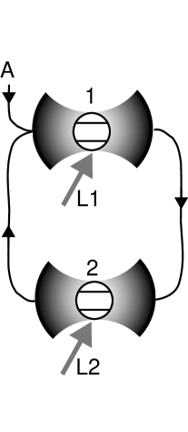
Figure 1: Schematic description of the considered set-up. Two distinct cavity $1$ and $2$ each containing a two-level atom are connected via optical fibers. Practically the output of each cavity enters the input of the other. Cavity $1$ also has an input off-resonant driving field ${\cal A}$. $L1$ and $L2$ represent resonant laser fields for local operations.

II The Model

We consider a very simple model consisting of two atoms, $1$ and $2$, placed in distant cavities and interacting with light fields in a dispersive way. The two cavities are then connected by optical fibers as depicted in Fig.1.

Interaction of atoms with light field in the dispersive regime can be accounted for by the following Hamiltonian HOL91

$$H_{int}=\chi A^{{\dagger}}A\sigma_{1}^{(z)}+\chi B^{{\dagger}}B\sigma_{2}^{(z)}\,,$$ (1)

where $A$, $B$ represent the relevant intracavity radiation modes belonging cavity $1$ and $2$ respectively. Furthermore, $\sigma_{j}^{(x)}=(\sigma_{j}+\sigma_{j}^{{\dagger}})$, $\sigma_{j}^{(y)}=-i(\sigma_{j}-\sigma_{j}^{{\dagger}})$ and $\sigma_{j}^{(z)}$ ($j=1,2$) are the Pauli operators associated to the atomic internal degree of freedom. The coupling constant $\chi$ (assumed, for the sake of simplicity, equal for the two atoms) is given by $g^{2}/\Delta$ with $g$ the dipole coupling and $\Delta$ the detuning from the internal transition HOL91 .

Suppose, for the moment, that there is no connection between the two cavities, and consider only the driving field of amplitude ${\cal A}$ at the first cavity. Then, the dynamics of the intracavity modes is described by the Langevin equations WM

$$\dot{A} = -\left(\frac{\gamma}{2}+i\Delta\right)A-i\chi A\sigma_{1}^{(z)}+\sqrt{\gamma}A_{in}+{\cal A}\,,$$ (2)

$$\dot{B} = -\left(\frac{\gamma}{2}+i\Delta\right)B-i\chi B\sigma_{2}^{(z)}+\sqrt{\gamma}B_{in}\,,$$ (3)

where $A_{in}$, $B_{in}$ represent vacuum input noise and $\gamma$ is the cavity decay rate (assumed equal for the two cavities) WM . For the moment we have ignored the spontaneous decay from the excited to the ground state of each atom. We will later present a case with feasible parameters in which this is possible.

If we now connect the output of the cavity $1$ with the input of cavity $2$, and the output of cavity $2$ with the input of cavity $1$ (as in Fig.1), we will have additional dynamical terms of the type WISE

$$\dot{A}=-\frac{\gamma}{2}A+\sqrt{\gamma}\,B^{\prime}_{out}\,,\quad\dot{B}=-\frac{\gamma}{2}B+\sqrt{\gamma}\,A^{\prime}_{out}\,,$$ (4)

where the subscript $out$ indicates the field outgoing a cavity, while the prime sign means the retardation effect due to the propagation of the field along the fiber, i.e., for a generic operator ${\cal O}$ it is ${\cal O}^{\prime}(t)\equiv{\cal O}(t-\tau)$ with $\tau$ the delay time. However, such effect can be described as the introduction of a phase factor WISE . Thus, adding the terms (4) to Eqs.(2) and taking into account the usual boundary conditions $A_{out}\,(B_{out})=\sqrt{\gamma}A\,(B)-A_{in}\,(B_{in})$ WM , we get

$$\dot{A} = -\left(\gamma+i\Delta\right)A+\gamma e^{i\phi_{12}}B-i\chi A\sigma_{1}^{(z)}$$ (5)

$$+\sqrt{\gamma}A_{in}-\sqrt{\gamma}e^{i\phi_{12}}B_{in}+{\cal A}\,,$$

$$\dot{B} = -\left(\gamma+i\Delta\right)B+\gamma e^{i\phi_{21}}A-i\chi B\sigma_{2}^{(z)}$$ (6)

$$+\sqrt{\gamma}B_{in}-\sqrt{\gamma}e^{i\phi_{21}}A_{in}\,,$$

where $\phi_{12}$ ($\phi_{21}$) is the phase introduced along the connection between the cavity $1$ ($2$) and the cavity $2$ ($1$). Such phases can be experimentally controlled. For the moment we ignore the loss effect in the fibers (i.e. assume lossless fibers). Later we will analyze the case for a lossy fiber linking the cavities.

Since we are interested on quantum effects at stationary regime, we are going to linearize our equations. First, let us write the steady state of the radiation fields by assuming $\gamma$, $\Delta>g$ (i.e. $\gamma>\chi$) and the expectation values of the vacuum fields $A_{in},B_{in}$ to be much smaller than the driving and cavity fields. It results

$$\alpha = \frac{{\cal A}(\gamma+i\Delta)}{(\gamma+i\Delta)^{2}-\gamma^{2}\exp\left[i\left(\phi_{12}+\phi_{21}\right)\right]}\,,$$ (7)

$$\beta = \gamma\alpha\exp\left(i\phi_{21}\right)/(\gamma+i\Delta)\,.$$ (8)

Notice that the limit $\Delta\to 0$ and $\phi_{12}+\phi_{21}\to 0$ cannot be taken, since due to the recycling effect the intracavity fields in such a case would explode.

Then, the linearized version of Eqs.(5) will be

$$\dot{a} = -\left(\gamma+i\Delta\right)a+\gamma e^{i\phi_{12}}b-i\chi\alpha\sigma_{1}^{(z)}$$ (9)

$$+\sqrt{\gamma}a_{in}-\sqrt{\gamma}e^{i\phi_{12}}b_{in}\,,$$

$$\dot{b} = -\left(\gamma+i\Delta\right)b+\gamma e^{i\phi_{21}}a-i\chi\beta\sigma_{2}^{(z)}$$ (10)

$$+\sqrt{\gamma}b_{in}-\sqrt{\gamma}e^{i\phi_{21}}a_{in}\,,$$

where we have used the replacement $A\,(B)\to\alpha\,(\beta)+a\,(b)$ and $a_{in}(b_{in})\equiv A_{in}(B_{in})$. From Eqs.(9) and (10), we can adiabatically eliminate the radiation fields to obtain expressions for $a$ and $b$ in terms of linear combinations of the Pauli operators $\sigma_{1}^{(z)}$ and $\sigma_{2}^{(z)}$. In doing so we can also neglect the noise terms for $1<<\gamma/\chi<<|\alpha|$. Inserting the expressions for $a$ and $b$ (and hence $A$ and $B$) in the Hamiltonian of Eq.(1), leads to an effective interaction Hamiltonian for the two atoms of the type

$$H_{eff}=2J\sigma_{1}^{(z)}\sigma_{2}^{(z)}\,,$$ (11)

with $J=\gamma\chi^{2}\Theta$, where we have assumed

$$\Theta = {\rm Im}\{\alpha^{*}\beta e^{i\phi_{12}}/((\gamma+i\Delta)^{2}-\gamma^{2}e^{i(\phi_{12}+\phi_{21})})\}\,,$$ (12)

$$= {\rm Im}\{\alpha\beta^{*}e^{i\phi_{21}}/((\gamma+i\Delta)^{2}-\gamma^{2}e^{i(\phi_{12}+\phi_{21})})\}\,.$$

In deriving the above Hamiltonian (11) we have neglected the self interaction terms since $[\sigma_{j}^{(z)}]^{2}=1$. There are also additional local terms in the Hamiltonian such as $\chi|\alpha|^{2}\sigma_{1}^{(z)}$ and $\chi|\beta|^{2}\sigma_{2}^{(z)}$. Notice that the Hamiltonian $H_{eff}$ is an Ising Hamiltonian whose spin-spin coupling $J$ scales as radiation pressure and goes to zero for $\Delta\to 0$ and $\phi_{12}+\phi_{21}\to 0$.

We have thus managed to generate an effective Ising interaction between two distant two-level atoms with the upper and lower energy levels (say $|e\rangle_{j}$ and $|g\rangle_{j}$ with $j=1,2$) taking the place of up and down spins of the original Ising model. This interaction strength can be arbitrarily increased by increasing the strength of radiation in the cavities. This concludes the first part of our paper, we next proceed to investigate an application of this interaction to entangling the distant atoms.

III Entanglement

Gunlycke et al. have recently investigated thermal entanglement in the Ising model in an arbitrarily directed magnetic field gunlycke01 . In particular, it was shown in Ref.gunlycke01 that to get entanglement in the Ising model, it is necessary to have a magnetic field perpendicular to the $z$ direction. To this end, we apply local laser fields to each atom (L1 and L2 of Fig.1) such that the local Hamiltonian $H_{local}$ given by

$$H_{local}=B\sigma_{1}^{(x)}+B\sigma_{2}^{(x)},$$ (13)

acts on the atoms in addition to $H_{eff}$. It is also assumed that the local terms of the effective Hamiltonian ($\chi|\alpha|^{2}\sigma_{1}^{(z)}$ and $\chi|\beta|^{2}\sigma_{2}^{(z)}$) are fully cancelled by choosing an appropriate detuning of the local laser fields from the $|e\rangle_{j}\rightarrow|g\rangle_{j}$ transition. We choose $B=\eta J$, with $\eta\ll 1$ so that the earlier derivation of the effective Ising Hamiltonian is unaffected by the presence of these extra classical laser fields. Thus the total Hamiltonian of the system is

$$H_{tot}=H_{local}+H_{eff}.$$ (14)

The Hamiltonian $H_{tot}$ has the following eigenvectors:

$$|\psi_{1}\rangle = \frac{\eta}{2\sqrt{1+\eta^{2}+\sqrt{1+\eta^{2}}}}\left(|g\rangle_{1}|g\rangle_{2}+|e\rangle_{1}|e\rangle_{2}\right)$$

$$-\frac{1+\sqrt{1+\eta^{2}}}{2\sqrt{1+\eta^{2}+\sqrt{1+\eta^{2}}}}\left(|e\rangle_{1}|g\rangle_{2}+|g\rangle_{1}|e\rangle_{2}\right)\,,$$

$$|\psi_{2}\rangle = \frac{1}{\sqrt{2}}\left(|e\rangle_{1}|g\rangle_{2}-|g\rangle_{1}|e\rangle_{2}\right)\,,$$ (16)

$$|\psi_{3}\rangle = \frac{1}{\sqrt{2}}\left(|g\rangle_{1}|g\rangle_{2}-|e\rangle_{1}|e\rangle_{2}\right)\,,$$

$$|\psi_{4}\rangle = \frac{\eta}{2\sqrt{1+\eta^{2}-\sqrt{1+\eta^{2}}}}\left(|g\rangle_{1}|g\rangle_{2}+|e\rangle_{1}|e\rangle_{2}\right)$$

$$-\frac{1-\sqrt{1+\eta^{2}}}{2\sqrt{1+\eta^{2}-\sqrt{1+\eta^{2}}}}\left(|e\rangle_{1}|g\rangle_{2}+|g\rangle_{1}|e\rangle_{2}\right)\,,$$

with eigenvalues $E_{1}=-2\sqrt{B^{2}+J^{2}}$, $E_{2}=-2J$, $E_{3}=2J$ and $E_{4}=2\sqrt{B^{2}+J^{2}}$.

Let us now consider as initial state of the two atoms the ground state $|g\rangle_{1}|g\rangle_{2}$, then we can expand it over the eigenstates basis as

$$|\Psi(0)\rangle=|g\rangle_{1}|g\rangle_{2}=\sum_{j=1}^{4}C_{j}|\psi_{j}\rangle\,,$$ (18)

with

$$C_{1} = -\frac{\left(1-\sqrt{1+\eta^{2}}\right)\sqrt{1+\eta^{2}+\sqrt{1+\eta^{2}}}}{2\eta\sqrt{1+\eta^{2}}}\,,$$ (19)

$$C_{2} = 0\,,$$ (20)

$$C_{3} = \frac{1}{\sqrt{2}}\,,$$ (21)

$$C_{4} = \frac{\left(1+\sqrt{1+\eta^{2}}\right)\sqrt{1+\eta^{2}-\sqrt{1+\eta^{2}}}}{2\eta\sqrt{1+\eta^{2}}}\,.$$ (22)

The evolution of the state (18) under $H_{tot}$ will give

$$|\Psi(t)\rangle = C_{1}e^{2i\tau\sqrt{1+\eta^{2}}}|\psi_{1}\rangle$$ (23)

$$+C_{3}e^{-2i\tau}|\psi_{2}\rangle$$

$$+C_{4}e^{-2i\tau\sqrt{1+\eta^{2}}}|\psi_{4}\rangle\,,$$

where we have introduced the scaled time $\tau=Jt$.

In Fig.2 we have plotted the entanglement of formation $E$ (from the formula by Wootters wootters98 ) for the state (23) as a function of $\tau$. We note that $E$ can approach the maximum value $1$ before diminishes. Its behavior is quasiperiodic as we are considering Hamiltonian dynamics with incommensurable frequencies. As soon as $E$ reaches a value $\simeq 1$ we can suppose to turn off $H_{local}$ (or $H_{tot}$) and leave the atoms in a maximally entangled states. Notice, from Eq.(23), that entanglement does not directly depend on the interaction strength, but rather on the ratio $B/J$. As a consequence $\eta$ determines the value of time for which the maximal entanglement ($E_{\mbox{max}}$) is reached. Setting $\tau_{*}$ as the smaller value of $\tau$ such that $E\approx E_{\mbox{max}}(\eta)\approx 1$, the inset of Fig.2 shows how $\tau_{*}$ increases by diminishing the value of $\eta$.

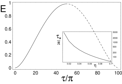
Figure 2: The figure shows the plot of the amount $E$ of entanglement between the distant atoms versus the scaled time $\tau$ for $\eta=0.1$. The inset shows, on a $\log$ scale, the time $\tau_{*}$ versus $\eta$.

IV Discussion

We have completely eliminated the optical field in the process of deriving the effective Hamiltonian. In doing that we have also neglected the losses along the fibers. We now examine what happens if the fiber is lossy. The important effect of a lossy fiber is that the primed fields $A^{{}^{\prime}}_{out}$ and $B^{{}^{\prime}}_{out}$ also have a damping term (say $\exp{(-\Gamma_{f})}$) in addition to the phase factor $\exp{(i\phi_{12})}$ relative to their unprimed counterparts. Hence we should be able to model the effect of a lossy fiber phenomenologically by replacing $\exp{(i\phi_{12})}$ and $\exp{(i\phi_{21})}$ by $\exp{(i\phi_{12}-\Gamma_{f}}$ and $\exp{(i\phi_{21}-\Gamma_{f})}$ respectively in Eqs.(5) to (11). When this replacement is done, only the dependence of $a$ on $\sigma_{2}^{(z)}$ and of $b$ on $\sigma_{1}^{(z)}$ is affected ($a$ and $b$ still depend in the same way on the local terms). The dependence of $J$ on $\Gamma_{f}$ is the found, in general, to be quite complicated (depends on the explicit values of $\gamma,\Delta,\phi_{12}$ and $\phi_{21}$). However, if we make the simplifying assumption that $\Delta>>\gamma$, then $J$ is simply replaced by $J\exp{(-2\Gamma_{f})}$. In the typical optical fibers used today, the loss rates are as low as $0.35$ dB per kilometer (this data is from a quantum communication experiment with photons gisin ). This translates to $\Gamma_{f}\approx 0.08$ for a fiber of one kilometer (separating cavities by the same distance). Then the coupling strength $J$ between the atoms is about $92$ percent of that estimated by Eq.(11).

Finally, once generated, entanglement may have a stability problem due to the atomic decay from the excited states. However, one can deal this problem by using, as $|e\rangle$ and $|g\rangle$, Zeeman ground state levels in a $\Lambda$ configuration Parkins93 . This guarantees long lived states and its use has been already proposed within quantum computation Pel95 . A recent experiment with atoms in optical cavities has used precisely this type of atomic system kuhn and we will estimate the feasibility of our proposal by slightly modifying the parameters of that experiment. The strength $\chi$ of our scheme is given in terms of two single photon Rabi frequencies $g$ and $\Omega$ and an atomic detuning $\Delta_{a}$ (different from our cavity detuning $\Delta$) of Ref.kuhn as $\chi=g\Omega/\Delta_{a}$. The parameters of the experiment of Ref.kuhn are $(g,\Omega,\Delta_{a},\gamma)=2\pi(2.5,8,-20,1.25)$ MHz. We increase $\gamma$ five times, which is easy to do (higher cavity decay rate) and choose $\Delta<<\gamma$ and $\phi_{12}=\phi_{21}=\pi/4$ for simplifying the expression of $J$ (these are not necessary). Then we have $J\approx\chi^{2}\bar{n}/2\gamma\approx\bar{n}/2$ MHz (where $\bar{n}=|\alpha|^{2}$ is the number of photons in the first cavity). Thus with $\bar{n}\sim 50-100$, we already have $J\sim 25-50$MHz, which is indeed a strength of interaction comparable to usual atom-light interaction strength in cavities.

V Conclusions

In conclusion, we have presented a scheme for generating an Ising interaction between distant atoms. Such a scheme has greater potential than any scheme that merely entangles the distant atoms. For example, a direct interaction can be used to implement a two qubit logic gate between the distant atoms. The strength of the coupling can be made arbitrary by pumping more or less radiation into any of the cavities. This is a result of using off-resonant coupling, between each atom and its cavity mode. The coupling of light with any general macroscopic object, called “ponderomotive” coupling (see Refs.mancini01 for its applications in the context of entanglement) is of the same type. Thus our entangling scheme could potentially be extended to generate thermal entanglement for macroscopic objects pond .

References

- (1) C. H. Bennett and D. P. DiVincenzo, Nature 404, 247 (2000).
- (2) J. I. Cirac et al., Phys. Rev. Lett. 78, 3221 (1997); S. J. van Enk et al., Phys. Rev. Lett. 78, 4293 (1997);
- (3) T. Pellizzari, Phys. Rev. Lett. 79, 5242 (1997); S. J. van Enk et al., Phys. Rev. A 59, 2659 (1999).
- (4) S. J. van Enk et al., Phys. Rev. Lett. 79, 5178 (1997)
- (5) A. Sørensen and K. Mølmer, Phys. Rev. A 58, 2745 (1998).
- (6) S. Bose et. al., Phys. Rev. Lett. 83, 5158 (1999); M. B. Plenio, et. al., Phys. Rev. A 59, 2468 (1999).
- (7) A. S. Parkins and H. J. Kimble, Phys. Rev. A 61, 052104 (2000).
- (8) S. Mancini and S. Bose, Phys. Rev. A 64, 032308 (2001).
- (9) L.-M. Duan, Phys. Rev. Lett. 88, 170402 (2002).
- (10) L.-M. Duan and H. J. Kimble, Phys. Rev. Lett. 90, 253601 (2003).
- (11) C. Simon and W. T. M. Irvine, Phys. Rev. Lett. 91, 110405 (2003).
- (12) S. Clark et. al., Phys. Rev. Lett. 91, 177901 (2003).
- (13) D.E. Browne et. al., Phys. Rev. Lett. 91, 067901 (2003).
- (14) M. J. Bremner et. al., Phys. Rev. Lett. 89, 247902 (2002).
- (15) M. J. Holland, et al., Phys. Rev. Lett. 67, 1716 (1991); see also appendix M of Quantum Optics in Phase Space, W. P. Schleich (Wiley, Berlin, 2001).
- (16) D. F. Walls and G. J. Milburn, Quantum Optics, (springer, Berlin, 1995).
- (17) H. M. Wiseman and G. J. Milburn, Phys. Rev. A 49, 4110 (1994).
- (18) D. Gunlycke et. al., Phys. Rev. A 64, 042302 (2001) .
- (19) W. K. Wootters, Phys. Rev. Lett 80, 2245 (1998).
- (20) W. Tittel et al., Phys. Rev. A 57, 3229 (1998).
- (21) A. S. Parkins, et al., Phys. Rev. Lett. 71, 3095 (1993).
- (22) T. Pellizzari, et al., Phys. Rev. Lett. 75, 3788 (1995).
- (23) A. Kuhn, M. Hennrich, and G. Rempe Phys. Rev. Lett. 89, 067901 (2002).
- (24) S. Mancini, et al., Phys. Rev. Lett. 88, 120401 (2002); Eur. J. Phys. D 22, 417 (2003).