Evolution of entanglement under echo dynamics

Abstract

Echo dynamics and fidelity are often used to discuss stability in quantum information processing and quantum chaos. Yet fidelity yields no information about entanglement, the characteristic property of quantum mechanics. We study the evolution of entanglement in echo dynamics. We find qualitatively different behavior between integrable and chaotic systems on one hand and between random and coherent initial states for integrable systems on the other. For the latter the evolution of entanglement is given by a classical time scale. Analytic results are illustrated numerically in a Jaynes Cummings model.

More than a century ago J. Loschmidt, in his discussions with L. Bolzmann illustrating irreversibility in a gas, suggested to invert the velocity of each atom individually in order to revert to the initial situation. Recently Loschmidt echoes have been of great interest in the control of quantum information processing Nielsen . As entanglement is the essential property of quantum mechanics, in the present paper we analyze the Loschmidt echo appearing in the entanglement of two quantum systems. As a measure of entanglement we use purity Zurek and show analytically as well as numerically that for classically integrable systems the purity decays as $1-c_{\rm In}t^{2}$, whereas for a classically chaotic system the decay after the Zeno time scale is described by $1-c_{\rm ch}t$. For a coherent state the constant $c_{\rm In}$ is independent of $\hbar$. For chaotic systems (or random initial states in integrable systems) this constant on the other hand is proportional to $1/{\hbar^{2}}$, thus defining quite different time scales.

Zurek Zurek proposed to use the rate of decoherence as a characteristic of chaos in quantum mechanics and this is occasionally re-interpreted in terms of entanglement Nemes between different parts of a closed quantum system. Such studies were limited to forward time evolution. Yet the insensitivity of quantum mechanics to small changes in initial conditions has been a basic difficulty in the introduction of the concepts of chaos to this field, and the idea to use sensitivity to perturbations in the time evolution Peres has emerged recently as one of the tools of choice to overcome this difficulty Jalabert ; Ktop . Specifically all these authors use fidelity, i.e. the correlation function between a quantum state evolving under the action of two Hamiltonians differing by a perturbation, which is equivalent to the autocorrelation function under echo dynamics. Since fidelity measures irreversibility of a full quantum state under the echo, it is also desirable to undertand irreversibility of a less restrictive quantity like entanglement. A recent study in spin chains Spinecho , more related to quantum computing, revealed no qualitative difference between fidelity and the evolution of entanglement under echo dynamics as measured conveniently by purity there denoted as purity-fidelity. This system allows no classical analogue, and by consequence no coherent states. Yet these we shall show to be essential to recover results analogue to the ones of Zurek and Nemes Zurek ; Nemes . Based on the idea that a partial trace simulates decoherence our results lead to the conjecture that Zureks result holds exclusively for coherent states in the central system, i.e. that we may not expect faster decoherence for chaotic central systems than for integrable ones, if we use random states that are more relevant to quantum information.

To implement this idea we have to consider systems with at least two degrees of freedom to allow for entanglement and a well defined classical limit $\hbar\to 0$. The (unperturbed) Hamiltonian will contain a parameter permitting a transition from order to chaos, and will typically couple the two degrees of freedom. A perturbation is then defined to obtain a second similar Hamiltonian. We give general results for entanglement under echo-dynamics starting from an initial product (dis-entangled) state. To illustrate our results we use the Jaynes Cummings (JC) model Jaynes&Cummings . The usual co-rotating (integrable) version of this model has great practical importance in atomic physics and illustrates the $\hbar$ independent evolution of entanglement for coherent states. For the arguments involving the chaotic dynamics we include counter-rotating terms Nemes ; Debergh to construct a toy model that allows for chaos. Even this model may not be entirely unrealistic for atoms in a Paul trap in a driven field, as standard papers seek conditions where this term is smallCirac .

For general considerations and analytic calculations techniques of linear response developed originally for the evaluation of fidelity Ktop are extended to calculate purity-fidelity in terms of time correlation functions of the perturbation. In the case of coherent states we could carry the evaluation of linear response one step further using it in a semi-classical framework that relates the decay rates directly to the stability matrix of the orbit along which the packet evolves.

We consider the unitary time evolution given by the echo operator $M_{\delta}(t)=U^{\dagger}_{\delta}(t)U(t)$. Here $U(t)$ is generated by some unperturbed Hamiltonian $H$ as $U(t)=e^{-iHt/\hbar}$ and similarly $U_{\delta}(t)=e^{-i(H+\delta V)t/\hbar}$, where $V$ is the perturbation with strength $\delta$. It is useful to rewrite the echo operator as time-ordered product Ktop in the interaction picture

$$M_{\delta}(t)=\hat{\cal T}\exp\left({\rm i}\Sigma(t)\delta/\hbar\right),$$ (1)

where $\Sigma(t):=\int_{0}^{t}{V(\tau)d\tau}$ with $V(t):=U^{\dagger}(t)VU(t)$. This operator shall act on a composite system with the Hilbert space ${\cal H}={\cal H}_{1}\otimes{\cal H}_{2}$, consisting of two factors with dimensions $N_{1}$ and $N_{2}$, which we may look upon as a “central system” and an “environment”. We are interested only in information about the subsystem $1$ which is contained in a reduced density matrix $\rho_{1}(t):={\rm tr_{2}}\rho(t)$, $\rho(t)=|\psi(t)\rangle\langle\psi(t)|$. We shall study the purity-fidelity Spinecho $F_{P}(t):={\,{\rm tr}}_{1}[\rho_{1}(t)]^{2}$ as a measure of factorizability of a joint state $|\psi(t)\rangle=M_{\delta}(t)|\psi(0)\rangle$. We choose this quantity rather than some entropy because of its simple analytic dependence on $\rho_{1}(t)$. Here the partial traces with indices 1 and 2 are taken in the corresponding factor spaces and the reduced density matrix is acting on the first factor space. We always assume that we start with a factorized state at $t=0$, i.e. $F_{P}(0)=1$. For comparison we shall also use the fidelity $|F(t)|^{2}=|\langle\psi(0)|M_{\delta}(t)|\psi(0)\rangle|^{2}$.

Expanding the echo operator (1) in $\delta$, we get Ktop

$$|F(t)|^{2} = 1-\delta^{2}\hbar^{-2}C(t)+\cdots,$$ (2)

$$C(t) := \langle\Sigma^{2}(t)\rangle-\langle\Sigma(t)\rangle^{2}.$$

Here $\langle.\rangle$ denotes an expectation in the product initial state $|\psi(0)\rangle=|1,1\rangle$ with the abbreviation $|i,\nu\rangle:=|i\rangle_{1}\otimes|\nu\rangle_{2}$. The same techniques yield for purity-fidelity

$$F_{\rm P}(t) = 1-2\delta^{2}\hbar^{-2}\left\{C(t)-D(t)\right\}+\cdots,$$ (3)

$$D(t) := \sum_{\nu\neq 1}|\langle 1,\nu|\Sigma(t)|1,1\rangle|^{2}+\sum_{i\neq 1}{|\langle i,1|\Sigma(t)|1,1\rangle|^{2}}$$

For both series to converge it is sufficient to use a bounded perturbation operator $V$, but we expect the linear response formula to be a good approximation for a much wider class of perturbations. The somewhat unusual correlation function $D(t)$ contains only off-diagonal matrix elements of the operator $\Sigma(t)$ and determines the difference between $F_{P}(t)$ and $|F(t)|^{4}$. From expansions (2,3) we can see that the decay is determined by time correlation functions of the perturbation. The stronger the decay of correlation functions $\langle\psi|V(t)V(t^{\prime})|\psi\rangle$ as $|t-t^{\prime}|$ grows, the slower is the increase of $C(t)$ and the slower is the decay of $F(t)$ and $F_{\rm P}(t)$.

We limit our discussion to systems which have a classical limit. For such systems chaos typically implies decay of the time correlation functions of the perturbation observable (i.e. mixing), while regular motion implies non-ergodic behavior. Fidelity decay for both situations is discussed in Ref. Ktop . Under rather general assumptions one finds exponential decay for chaotic dynamics

$$|F(t)|^{2}=\exp{(-t/\tau_{\rm em})},\qquad\tau_{\rm em}=(2\sigma)^{-1}\hbar^{2}\delta^{-2},$$ (4)

where a diffusion coefficient $\sigma:=\lim_{t\to\infty}C(t)/(2t)$ is independent of the initial state $|\psi(0)\rangle$ [for sufficiently long times, typically $t\gg\log 1/\hbar$]. In classically regular situation the fidelity exhibits a quadratic decay in the leading order in $\delta$ even for long times, since $C(t)\to\bar{c}t^{2}$, where $\bar{c}$ depends on the structure of the initial state. For a coherent initial state we find a Gaussian decay of fidelity

$$|F(t)|^{2}=\exp{(-(t/\tau_{\rm ne})^{2})},\qquad\tau_{\rm ne}=\bar{c}^{-1/2}\hbar\delta^{-1}$$ (5)

with $\bar{c}\propto\hbar$ Ktop . It is worth to stress that in the regime of linear response (small $\delta$) formulae (4,5) agree with Eqs. (2,3) from which the time scales $\tau_{\rm em},\tau_{\rm ne}$ are obtained.

As for purity-fidelity of chaotic systems, one may argue that $\Sigma(t)$ should look like a random matrix so the term $D(t)$ should be small compared to $C(t)$ in (3), namely $D(t)/C(t)\sim 1/N_{1}+1/N_{2}$ because of the smaller number of terms involved in the sums. Thus, if both dimensions $N_{1,2}$ grow as $\hbar\to 0$ one expects in the asymptotic regime that $F_{\rm P}(t)=|F(t)|^{4}=\exp(-2t/\tau_{\rm em})$, and does not significantly depend on the initial state. In particular this also holds for coherent initial states. Using similar arguments for regular dynamics but a random initial state one again sees that $F_{\rm P}(t)$ follows $|F(t)|^{4}$ closely Spinecho .

Yet for coherent states and regular classical dynamics this is not the case because the term $D(t)$ is not negligible. We show that the difference $C(t)-D(t)$ cancels in the leading order in $\hbar$, i.e. $C(t)-D(t)\sim\hbar^{2}$, meaning that $F_{\rm P}(t)$ as compared to $|F(t)|^{2}$ decays on a qualitatively longer, $\hbar$-independent time scale $\tau^{\rm P}_{\rm ne}=K/\delta\sim\hbar^{-1/2}\tau_{\rm ne}$. This will be the main result of the present paper. In order to establish this we consider the evolution of a Gaussian wave-packet along a stable orbit $\vec{z}_{t}=(\vec{x}_{t},\vec{p}_{t})$ as $\langle\vec{x}|\psi(t)\rangle=C\exp(\frac{i}{\hbar}[(\vec{x}-\vec{x}_{t})\cdot A_{t}(\vec{x}-\vec{x}_{t})+\vec{p}_{t}\cdot\vec{x}])$, where the block-form of the complex $d\times d$ matrix

$$A_{t}=\begin{pmatrix}A_{11}&A_{12}\cr A_{21}&A_{22}\cr\end{pmatrix}$$ (6)

corresponds to obvious division of $d=d_{1}+d_{2}$ dimensional configuration space into $d_{1}$ and $d_{2}$ dimensional parts. $A_{t}$ is a ratio of two pieces of a classical monodromy matrix Heller so it is $\hbar$-independent. The purity of a reduced wave-packet $\rho(x_{1},x^{\prime}_{1})=\int dx_{2}\langle x_{1},x_{2}|\psi(t)\rangle\langle\psi(t)|x^{\prime}_{1},x_{2}\rangle$ is $F_{P}=\int dx_{1}dx^{\prime}_{1}|\rho(x_{1},x^{\prime}_{1})|^{2}=1$ if $A_{12}=A_{21}=0$ while in general we find $\hbar-$independent expression

$$F_{P}=(\det{\,{\rm Im}\,}A)\left|\begin{matrix}{\,{\rm Im}\,}A_{11}&\frac{\rm i}{2}A_{12}^{*}&0&-\frac{\rm i}{2}A_{12}\cr\frac{\rm i}{2}A_{21}^{*}&{\,{\rm Im}\,}A_{22}&-\frac{\rm i}{2}A_{21}&0\cr 0&-\frac{\rm i}{2}A_{12}&{\,{\rm Im}\,}A_{11}&\frac{\rm i}{2}A_{12}\cr-\frac{\rm i}{2}A_{21}&0&\frac{\rm i}{2}A_{21}^{*}&{\,{\rm Im}\,}A_{22}\cr\end{matrix}\right|^{-1/2}.$$

For classical echo dynamics, the covariance matrix $A=A_{t}$ is given by a linear stability analysis as $A=A_{0}+t\delta B$ for some matrix $B$, where $A_{0,12}=A_{0,21}=0$. Then purity-fidelity is $\hbar$-independent and can be evaluated in the leading orders as $F_{\rm P}(t)=1-(t\delta/K)^{2}+\ldots$.

We thus reach the following interesting conclusion: Both fidelity and purity-fidelity decay quadratically in integrable situations, while they decay linearly in chaotic ones, once we are beyond the Zeno time scale. Yet there is a very relevant difference in time scales themselves, if we discuss the purity of coherent rather than random states. For integrable systems purity-fidelity decays on an $\hbar$-independent scale. This leads to situations with very stable purity-fidelity, while the same perturbation generates decay of the fidelity of the coherent state as well as the decay of the purity-fidelity of a random state on much shorter time scales, dictated by the value of $\hbar$. Note though that for sufficiently small perturbations at fixed $\hbar$ the quadratic decline of purity-fidelity always prevails.

To illustrate these results we use the JC Hamiltonian including co- and counter-rotating terms for the chaotic case as

$$H=\hbar\omega a^{\dagger}a+\hbar\epsilon J_{\rm z}+\frac{\hbar}{\sqrt{2J}}(GaJ_{+}+G^{\prime}aJ_{-}+{\rm h.c.})$$ (7)

with standard boson operators $a,a^{\dagger}$, $[a,a^{\dagger}]=1$, and standard SU(2) generators $J_{\pm},J_{\rm z}$. We choose $\hbar=1/J$ ensuring that the classical limit is reached for $J\to\infty$ while the angular momentum $\hbar J=1$ is fixed. If either $G=0$ or $G^{\prime}=0$ the model is integrable with an additional invariant being the difference or the sum of quanta for the spin and the oscillator. In all calculations we used coherent initial states for the product system, i.e. direct product of coherent states of the oscillator, $|\alpha\rangle_{2}=e^{\alpha a^{\dagger}-\alpha^{*}a}|0\rangle_{2}$, and of the spin [SU(2)], $|\theta,\phi\rangle_{1}=(1+\tau\tau^{*})^{-J}\exp{(\tau J_{-})}|J,J\rangle$ with $\tau=e^{{\rm i}\phi}\tan{(\theta/2)}$ Agarwal81 .

For our numerics we fix $J=4$ and choose initial position of SU(2) coherent state at $(\theta,\phi)=(1,1)$ and for the oscillator at $\alpha=1.15$. The parameters in JC Hamiltonian are: (a) in chaotic regime $\omega=\epsilon=0.3$ and $G=G^{\prime}=1$, (b) in integrable regime $\omega=\epsilon=0.3$ and $G=1,G^{\prime}=0$. The corresponding classical Poincaré section shows a single practically ergodic component in the chaotic case (a) [at energy $E=1.0$ determined from the initial condition], whereas integrable case (b) [$E=0.63$] shows a generic family of invariant tori. The perturbation is realized by varying the parameter $\epsilon$ in JC Hamiltonian (7), also known as dephasing, so the (bounded) perturbation generator is $V=\hbar J_{\rm z}$.

We now show numerical results obtained by diagonalization in truncated Hilbert spaces. Stability of the calculation with respect to truncation was checked. Fig. 1 presents the correlation integrals $C(t)/t$ and $D(t)/t$ for chaotic and regular regimes. For chaotic dynamics (case a) the correlation integral converges after $t\approx 10$ to a well defined diffusion coefficient $\sigma=0.10$ with the D-term being of order $1/N_{1}+1/N_{2}\approx 1/4$. For regular dynamics (case b) and $t>10$ the correlation integral grows as $t^{2}$ due to a non-vanishing plateau $\bar{c}=0.046$ in the correlation function. In this case the difference $C(t)-D(t)$ is approximately $C(t)/J\propto\hbar^{2}$, which has been checked numerically also for larger $J\leq 24$, confirming $\hbar$-independent decay of $F_{\rm P}(t)$. The oscillations in these functions are not accounted for by the present theory, and are probably particular but interesting properties of the model. Whether they relate to oscillations seen in Nemes is an open question.

Figure 1: Correlation integrals $C(t)/t$ and $D(t)/t$ for regular (top two dotted curves) and chaotic regime (lower two solid curves). In both cases the upper curve is for $C(t)/t$ and the lower for $D(t)/t$. The horizontal dashed lines indicate $2\sigma=0.20$ (upper) and $0.20/4$ (lower), whereas the increasing ones have the slopes $\bar{c}=0.046$ (upper) and $(1-0.98/4)\bar{c}$ (lower).

Figure 2: Purity-Fidelity $F_{\rm P}(t)$ (main figure) and squared fidelity $|F(t)|^{4}$ (inset) in chaotic regime (solid curves) and in integrable regime (dotted curves), for $\delta=0.1$. The dashed lines indicate the linear and quadratic approximation respectively. Note the differences in vertical scales.

We first report a calculation with a strong perturbation $\delta=0.1$, that rapidly exceeds the realm of validity of linear response, in Fig. 2 where the main figure gives the purity-fidelity and the inset the fidelity. For the fidelity decay (inset) we find excellent agreement with the exponential decay (4) in a chaotic regime and a faster Gaussian decay in a regular regime (5), where the decay rates are fixed as above. However, for purity-fidelity we find already at $t\approx 20$, that the decay starts to be influenced by the saturation value of $F_{\rm P}(t\to\infty)\approx 1/(2J+1)$. Therefore purity-fidelity is higher for the integrable case than for the chaotic one not only at short times, as expected, but even at large times. This is relevant, because we shall next choose a weak perturbation $\delta=0.005$ to avoid this problem.

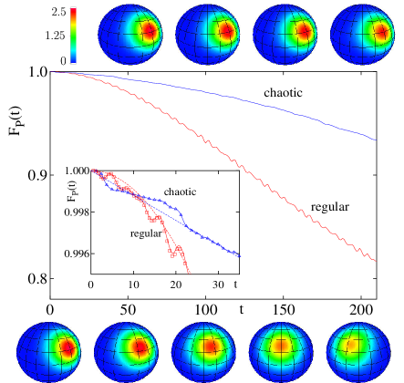
Figure 3: (Color) Echo dynamics for weak coupling: $\delta=0.005$. Square of the Wigner function for chaotic dynamics (top diagrams) and integrable dynamics as a function of time (bottom diagrams) at times corresponding to the axis. Color code: top left. Purity-fidelity is shown in the frame on the same time scale and for short times in the inset. Red curves give the integrable and blue curves the chaotic evolution. Full curves show the complete numerics, symbols the evaluation starting from the numerical correlation functions of Fig. 1 and dashed curves the linear or quadratic approximation.

We expect and find the crossover after a fairly short time. This calculation allows comparison with theory as well as an illustration of the evolution of the square of the Wigner function , corresponding to the reduced density matrix $\rho_{1}(t)$ for the angular momentum states on the sphere using the definition of Agarwal81 . Near the top and bottom of Fig. 3 we see this evolution for the chaotic and the integrable Hamiltonian respectively. In the center of the figure we plot the purity-fidelity on the same time scale as the Wigner functions in the main frame and an amplification of short times in the inset. We observe detailed agreement of numerics with results obtained from the numerical values of the correlation integrals (2,3) reproducing the oscillatory structure. From the same correlation integrals we obtained the coefficients for the linear and quadratic decay, which agree well if we discard the oscillations. We see a crossing of the two curves at $t=t^{*}_{\rm P}\approx 12$ for $F_{\rm P}$. This times are larger than the Zeno time ($\approx 1$) and indicate the competition of the decay rate and the decay shape as expected for a non-small value of $\hbar=1/4$. It is important to remember that the integral over the square of the Wigner function gives the purity and therefore the fading of the picture will be indicative of the purity decay. On the other hand the movement of the center is an indication of the rapid decay of fidelity (not shown in the figure).

In this letter we study the linearized behavior of the evolution of entanglement under echo dynamics for time-scales large compared to those of the quantum Zeno effect, but sufficiently short for the expansion to be valid. Similarly to the behavior of fidelity the decay of purity-fidelity is typically quadratic for non-mixing systems, and linear for mixing ones, the first situation arising for integrable systems and the second for chaotic ones. An interesting particular, but relevant case appears if we consider coherent initial states and integrable classical dynamics. In this case we have shown that purity-fidelity, still having a quadratic decay, can be computed classically in the leading order which is $\hbar$-independent, so the time scale for purity-fidelity decay of a coherent state is longer by a factor proportional to $\hbar^{-1/2}$ than the corresponding one for a random state. Coherent states in integrable systems are thus particularly long lived for semi-classical echo situations. On the other hand, for chaotic classical dynamics and coherent initial states we find that purity-fidelity is the same as for random states, and its decay will be slower than for either random or coherent initial states and integrable dynamics provided that time is sufficiently long or perturbation $\delta$ is sufficiently small.

We are grateful to W. Schleich for his extensive discussion of our manuscript. Financial support by the Ministry of Education, Science and Sports of Slovenia and from projects IN-112200, DGAPA UNAM, Mexico, 25192-E CONACYT Mexico and DAAD19-02-1-0086, ARO United States is gratefully acknowledged. TP and MŽ thank CIC, where this work was completed, for its hospitality.

References

- (1) M. A. Nielsen and I. L. Chuang Quantum Computation and Quantum information (Cambridge University Press, Cambridge 2000).
- (2) W. H. Zurek, Physics Today 44(10), 36 (1991); W. H. Zurek and J. P. Paz, Physica 83D, 300 (1995).
- (3) K. Furuya et al. Phys. Rev. Lett. 80, 5524 (1998); R. M. Angelo et al. Phys. Rev. A 64, 043801 (2001).
- (4) A. Peres, Phys. Rev. A 30, 1610 (1984).
- (5) H. M. Pastawski et al. Phys. Rev. Lett. 75, 4310 (1995); P. R. Levstein et al. J. Chem. Phys. 108, 2718 (1998); R. A. Jalabert and H. M. Pastawski, Phys. Rev. Lett. 86, 2490 (2001); Ph. Jacquod et al. Phys. Rev. E 64, 055203(R) (2001); N. R. Cerruti and S. Tomsovic, Phys. Rev. Lett. 88, 054103 (2002); F. M. Cucchietti et al. Phys. Rev. E 65 046209 (2002); D. A. Wisniacki and D. Cohen, Phys. Rev. E 66 046209 (2002); T. Kottos and D. Cohen, Europhys. Lett. 61 431 (2003).
- (6) T. Prosen and M. Žnidarič, J. Phys. A 35, 1455 (2002); T. Prosen, Phys. Rev. E 65, 036208 (2002).
- (7) T. Prosen and T. H. Seligman, J. Phys. A 35, 4707 (2002).
- (8) E. T. Jaynes and F. W. Cummings, Proc. IEEE 51, 89 (1963); M. Tavis and F. W. Cummings, Phys. Rev. 170, 379 (1968).
- (9) See, e.g., N. Debergh and A. B. Klimov, Int. J. Mod. Phys. A 16, 4057 (2001).
- (10) See, e.g., J. I. Cirac et al., Phys. Rev. Lett. 70, 762 (1993)
- (11) E. J. Heller, in Chaos and Quantum Physics, ed. A. Voros et al (North-Holland, Amsterdam 1991).
- (12) G. S. Agarwal, Phys. Rev. A 24, 2889 (1981).