Entangled states and collective nonclassical effects in two-atom systems

Abstract

We propose a review of recent developments on entanglement and non-classical effects in collective two-atom systems and present a uniform physical picture of the many predicted phenomena. The collective effects have brought into sharp focus some of the most basic features of quantum theory, such as nonclassical states of light and entangled states of multiatom systems. The entangled states are linear superpositions of the internal states of the system which cannot be separated into product states of the individual atoms. This property is recognized as entirely quantum-mechanical effect and have played a crucial role in many discussions of the nature of quantum measurements and, in particular, in the developments of quantum communications. Much of the fundamental interest in entangled states is connected with its practical application ranging from quantum computation, information processing, cryptography, and interferometry to atomic spectroscopy.

1 Introduction

A central topic in the current studies of collective effects in multi-atom systems are the theoretical investigations and experimental implementation of entangled states to quantum computation and quantum information processing [1]. The term entanglement, one of the most intriguing properties of multiparticle systems, was introduced by Schrödinger [2] in his discussions of the foundations of quantum mechanics. It describes a multiparticle system which has the astonishing property that the results of a measurement on one particle cannot be specified independently of the results of measurements on the other particles. In recent years, entanglement has become of interest not only for the basic understanding of quantum mechanics, but also because it lies at the heart of many new applications ranging from quantum information [3, 4], cryptography [5] and quantum computation [6, 7] to atomic and molecular spectroscopy [8, 9]. These practical implementations all stem from the realization that we may control and manipulate quantum systems at the level of single atoms and photons to store and transfer information in a controlled way and with high fidelity.

All the implementations of entangled atoms must contend with the conflict inherent to open systems. Entangling operations on atoms must provide strong coherent coupling between the atoms, while shielding the atoms from the environment in order to make the effect of decoherence and dissipation negligible. The difficulty of isolating the atoms from the environment is the main obstacle inhibiting practical applications of entangled states. The environment consists of a continuum of electromagnetic field modes surrounding the atoms. This gives rise to decoherence that leads to the loss of information stored in the system. However, it has been recognised that the collective properties of multi-atom systems can alter spontaneous emission compared with the single atom case. As it was first pointed out by Dicke [10], the interaction between the atomic dipoles could cause the multiatom system to decay with two significantly different, one enhanced and the other reduced, spontaneous emission rates. The presence of the reduced spontaneous emission rate induces a reduction of the linewidth of the spectrum of spontaneous emission [11, 12]. This reduced (subradiant) spontaneous emission implies that the multi-atom system can decohere slower compared with the decoherence of individual atoms.

Several physical realisations of entangled atoms have been proposed involving trapping and cooling of a small number of ions or neutral atoms [13, 14, 15, 16]. This is the case with the lifetime of the superradiant and subradiant states that have been demonstrated experimentally with two barium ions confined in a spherical Paul trap [13, 14]. The reason for using cold trapped atoms or ions is twofold. On the one hand, it has been realised that the trapped atoms are essentially motionless and lie at a known and controllable distance from one another, permitting qualitatively new studies of interatomic interactions not accessible in a gas cell or an atomic beam [17]. The advantage of the trapped atoms is that it allows to separate collective effects, arising from the correlations between the atoms, from the single-atom effects. On the other hand it was discovered that cold trapped atoms can be prepared in maximally entangled states that are isolated from its environment [18, 19, 20, 21, 22].

An example of maximally entangled states in a two-atom system are the superradiant and subradiant states, which correspond to the symmetric and antisymmetric combinations of the atomic dipole moments, respectively. These states are created by the interaction between the atoms and are characterized by different spontaneous decay rates that the symmetric state decays with an enhanced, whereas the antisymmetric state decays with a reduced spontaneous emission rate. The reduced spontaneous emission rate of the antisymmetric state implies that the state is weakly coupled to the environment. For the case of the atoms confined into the region much smaller than the optical wavelength (Dicke model), the antisymmetric state is completely decoupled from the environment, and therefore can be regarded as a decoherence-free state.

Another particularly interesting entangled states of a two-atom system are two-photon entangled states that are superpositions of only those states of the two-atom system in which both or neither of the atoms is excited. These states have been known for a long time as pairwise atomic states or multi-atom squeezed states [23, 24, 25, 26, 27, 28]. The two-photon entangled states cannot be generated by a coherent laser field coupled to the atomic dipole moments. The states can be created by a two-photon excitation process with nonclassical correlations that can transfer the population from the two-atom ground state to the upper state without populating the intermediate one-photon states. An obvious candidate for the creation of the two-photon entangled states is a broadband squeezed vacuum field which is characterised by strong nonclassical two-photon correlations [29, 30, 31].

One of the fundamental interests in collective atomic effects is to demonstrate creation of entanglement on systems containing only two atoms. A significant body of work on preparation of a two-atom system in an entangled state has accumulated, and two-atom entangled states have already been demonstrated experimentally using ultra cold trapped ions in free space [14, 32] and cavity quantum electrodynamics (QED) schemes [33, 34]. In the free space situation, the collective effects arise from the interaction between the atoms through the vacuum field that the electromagnetic field produced by one of the atoms influences the dipole moment of the another atom. This leads to an additional damping and a shift of the atomic levels that both depend on the interatomic separation. In the cavity QED scheme, the atoms interact through the cavity mode and in a good cavity limit, photons emitted by one of the atoms are almost immediately absorbed by the another atom. In this case, the system behaves like the Dicke model. Moreover, the strong coupling of the atoms to the cavity mode prevents the atoms to emit photons to the vacuum modes different from the cavity mode that reduces decoherence.

Recently, the preparation of correlated superposition states in multi-atom system has been performed using a quantum nondemolition (QND) measurement technique [35]. Osnaghi et al. [36] have demonstrated coherent control of two Rydberg atoms in a non-resonant cavity environment. By adjusting the atom-cavity detuning, the final entangled state could be controlled, opening the door to complex entanglement manipulations [37]. Several proposals have also been made for entangling atoms trapped in distant cavities [38, 39, 40, 41, 42, 43], or in a Bose-Einstein condensate [44, 45]. In a very important experiment, Schlosser et al. [46] succeeded in confining single atoms in microscopic traps, thus enhancing the possibility of further progress in entanglement and quantum engineering.

This review is concerned primarily with two-atom systems, since it is generally believed that entanglement of only two microscopic quantum systems (two qubits) is essential to implement quantum protocols such as quantum computation. Some description of the theoretical tools required for prediction of entanglement in atomic systems is appropriate. Thus, we propose to begin the review with an overview of the mathematical apparatus necessary for describing the interaction of atoms with the electromagnetic field. We will present the master equation technique and, in addition, we also describe a more general formalism based on the quantum jump approach. We review theoretical and experimental schemes proposed for the preparation of two two-level atoms in an entangled state. We will also relate the atomic entanglement to nonclassical effects such as photon antibunching, squeezing and sub-Poissonian photon statistics. In particular, we consider different schemes of generation of entangled and nonclassical states of two identical as well as nonidentical atoms. The cases of maximally and non-maximally entangled states will be considered and methods of detecting of particular entangled and nonclassical state of two-atom systems are discussed. Next, we will examine methods of preparation of a two-atom system in two-photon entangled states. Finally, we will discuss methods of mapping of the entanglement of light on atoms involving collective atomic interactions and squeezing of the atomic dipole fluctuations.

2 Time evolution of a collective atomic system

The standard formalism for the calculations of the time evolution and correlation properties of a collective system of atoms is the master equation method. In this approach, the dynamics are studied in terms of the reduced density operator $\hat{\rho}_{A}$ of the atomic system interacting with the quantized electromagnetic (EM) field regarded as a reservoir [47, 48, 49]. There are many possible realizations of reservoirs. The typical reservoir to which atomic systems are coupled is the quantized three-dimensional multimode field. The reservoir can be modelled as a vacuum field whose the modes are in ordinary vacuum states, or in thermal states, or even in squeezed vacuum states. The major advantage of the master equation is that it allows us to consider the evolution of the atoms plus field system entirely in terms of average values of atomic operators. We can derive equations of motion for expectation values of an arbitrary combination of the atomic operators, and solve these equations for time-dependent averages or the steady-state. Another method is the quantum jump approach. This is based on the theory of quantum trajectories [50], which is equivalent to the Monte Carlo wave-function approach [51, 52], and allows to predict all possible trajectories of a single quantum system which stochastically emits photons. Both methods, the master equation and quantum jumps approaches lead to the same final results of the dynamics of an atomic system, and are widely used in quantum optics.

2.1 Master equation approach

We first give an outline of the derivation of the master equation of a system of $N$ non-identical nonoverlapping atoms coupled to the quantized three-dimensional EM field. This derivation is a generalisation of the master equation technique, introduced by Lehmberg [47], to the case of non-identical atoms interacting with a squeezed vacuum field. Useful references on the derivation of the master equation of an atomic system coupled to an ordinary vacuum are the books of Louisell [48] and Agarwal [49]. The atoms are modelled as two-level systems, with excited state $|{e_{i}}\rangle$, ground state $|{g_{i}}\rangle$, transition frequency $\omega_{i}$, and transition dipole moments $\vec{\mu}_{i}$. We assume that the atoms are located at different points $\vec{r}_{1},\dots\vec{r}_{N}$, have different transition frequencies $\omega_{1}\neq\omega_{2}\neq\dots\neq\omega_{N}$, and different transition dipole moments $\vec{\mu}_{1}\neq\vec{\mu}_{2}\neq\dots\neq\vec{\mu}_{N}$.

In the electric dipole approximation, the total Hamiltonian of the combined system, the atoms plus the EM field, is given by

$$\hat{H} = \sum_{i=1}^{N}\hbar\omega_{i}S_{i}^{z}+\sum_{\vec{k}s}\hbar\omega_{k}\left(\hat{a}_{\vec{k}s}^{\dagger}\hat{a}_{\vec{k}s}+\frac{1}{2}\right)$$ (1)

$$- i\hbar\sum_{\vec{k}s}\sum_{i=1}^{N}\left[\vec{\mu}_{i}\cdot\vec{g}_{\vec{k}s}\left(\vec{r}_{i}\right)\left(S_{i}^{+}+S_{i}^{-}\right)\hat{a}_{\vec{k}s}-{\rm H.c.}\right]\ ,$$

where $S_{i}^{+}=|{e_{i}}\rangle\langle{g_{i}}|$ and $S_{i}^{-}=|{g_{i}}\rangle\langle{e_{i}}|$ are the dipole raising and lowering operators, $S_{i}^{z}=\left(|{e_{i}}\rangle\langle{e_{i}}|-|{g_{i}}\rangle\langle{g_{i}}|\right)/2$ is the energy operator of the $i$th atom, $\hat{a}_{\vec{k}s}$ and $\hat{a}_{\vec{k}s}^{\dagger}$ are the annihilation and creation operators of the field mode $\vec{ks}$, which has wave vector $\vec{k}$, frequency $\omega_{k}$ and the index of polarization $s$. The coupling constant

$$\vec{g}_{\vec{k}s}\left(\vec{r}_{i}\right)=\left(\frac{\omega_{k}}{2\epsilon_{0}\hbar V}\right)^{\frac{1}{2}}\bar{e}_{\vec{k}s}e^{i\vec{k}\cdot\vec{r}_{i}}\ ,$$ (2)

is the mode function of the three-dimensional vacuum field, evaluated at the position $\vec{r}_{i}$ of the $i$th atom, $V$ is the normalization volume, and $\bar{e}_{\vec{k}s}$ is the unit polarization vector of the field.

The atomic dipole operators, appearing in Eq. (1), satisfy the well-known commutation and anticommutation relations

$$\left[S_{i}^{+},S_{j}^{-}\right]=2S_{i}^{z}\delta_{ij}\ ,\quad\left[S_{i}^{z},S_{j}^{\pm}\right]=\pm S_{i}^{\pm}\delta_{ij}\ ,\quad\left[S_{i}^{+},S_{j}^{-}\right]_{+}=\delta_{ij}\ ,$$ (3)

with $\left(S_{i}^{\pm}\right)^{2}\equiv 0$.

While this is straightforward, it is often the case that it is simpler to work in the interaction picture in which the Hamiltonian (1) evolves in time according to the interaction with the vacuum field. Therefore, we write the total Hamiltonian (1) as

$$\hat{H} = \hat{H}_{0}+\hat{H}_{I}\ ,$$ (4)

where

$$\hat{H}_{0} = \sum_{i=1}^{N}\hbar\omega_{i}S_{i}^{z}+\sum_{\vec{k}s}\hbar\omega_{k}\left(\hat{a}_{\vec{k}s}^{\dagger}\hat{a}_{\vec{k}s}+\frac{1}{2}\right)\ ,$$ (5)

is the Hamiltonian of the non-interacting atoms and the EM field, and

$$\hat{H}_{I} = -i\hbar\sum_{\vec{k}s}\sum_{i=1}^{N}\left[\vec{\mu}_{i}\cdot\vec{g}_{\vec{k}s}\left(\vec{r}_{i}\right)\left(S_{i}^{+}+S_{i}^{-}\right)\hat{a}_{\vec{k}s}-{\rm H.c.}\right]\ ,$$ (6)

is the interaction Hamiltonian between the atoms and the EM field.

The Hamiltonian $\hat{H}_{0}$ transforms the total Hamiltonian (1) into

$$\hat{H}\left(t\right) = e^{i\hat{H}_{0}t/\hbar}\left(\hat{H}-\hat{H}_{0}\right)e^{-i\hat{H}_{0}t/\hbar}=\hat{V}\left(t\right)\ ,$$ (7)

where

$$\hat{V}\left(t\right) = -i\hbar\sum_{\vec{k}s}\sum_{i=1}^{N}\left\{\vec{\mu}_{i}\cdot\vec{g}_{\vec{k}s}\left(\vec{r}_{i}\right)S_{i}^{+}\hat{a}_{\vec{k}s}e^{-i\left(\omega_{k}-\omega_{i}\right)t}\right.$$ (8)

$$\left.+\vec{\mu}_{i}\cdot\vec{g}_{\vec{k}s}\left(\vec{r}_{i}\right)S_{i}^{-}\hat{a}_{\vec{k}s}e^{-i\left(\omega_{k}+\omega_{i}\right)t}-{\rm H.c.}\right\}\ .$$

We will consider the time evolution of the collection of atoms interacting with the vacuum field in terms of the density operator $\hat{\rho}_{AF}$ characterizing the statistical state of the combined system of the atoms and the vacuum field. The time evolution of the density operator of the combined system obeys the equation

$$\frac{\partial}{\partial t}\hat{\rho}_{AF}=\frac{1}{i\hbar}\left[\hat{H},\hat{\rho}_{AF}\right]\ .$$ (9)

Transforming Eq. (9) into the interaction picture with

$$\tilde{\hat{\rho}}_{AF}\left(t\right)=e^{i\hat{H}_{0}t/\hbar}\hat{\rho}_{AF}e^{-i\hat{H}_{0}t/\hbar}\ ,$$ (10)

we find that the transformed density operator satisfies the equation

$$\frac{\partial}{\partial t}\tilde{\hat{\rho}}_{AF}\left(t\right)=\frac{1}{i\hbar}\left[\hat{V}\left(t\right),\tilde{\hat{\rho}}_{AF}\left(t\right)\right]\ ,$$ (11)

where the interaction Hamiltonian $\hat{V}\left(t\right)$ is given in Eq. (8).

Equation (11) is a simple differential equation which can be solved by the iteration method. For the initial time $t=0$, the integration of Eq. (11) leads to the following first-order solution in $\hat{V}\left(t\right)$:

$$\tilde{\hat{\rho}}_{AF}\left(t\right)=\tilde{\hat{\rho}}_{AF}\left(0\right)+\frac{1}{i\hbar}\int_{0}^{t}dt^{\prime}\left[\hat{V}\left(t^{\prime}\right),\tilde{\hat{\rho}}_{AF}\left(t^{\prime}\right)\right]\ .$$ (12)

Substituting Eq. (12) into the right side of Eq. (11) and taking the trace over the vacuum field variables, we find that to the second order in $\hat{V}\left(t\right)$ the reduced density operator of the atomic system $\hat{\rho}_{A}\left(t\right)={\rm Tr}_{F}\tilde{\hat{\rho}}_{AF}\left(t\right)$ satisfies the integro-differential equation

$$\frac{\partial}{\partial t}\hat{\rho}_{A}\left(t\right) = \frac{1}{i\hbar}{\rm Tr}_{F}\left[\hat{V}\left(t\right),\tilde{\hat{\rho}}_{AF}\left(0\right)\right]$$ (13)

$$- \frac{1}{\hbar^{2}}\int_{0}^{t}dt^{\prime}{\rm Tr}_{F}\left\{\left[\hat{V}\left(t\right),\left[\hat{V}\left(t^{\prime}\right),\tilde{\hat{\rho}}_{AF}\left(t^{\prime}\right)\right]\right]\right\}\ .$$

We choose an initial state with no correlations between the atomic system and the vacuum field, which allows us to factorize the initial density operator of the combined system as

$$\tilde{\hat{\rho}}_{AF}\left(0\right)=\hat{\rho}_{A}\left(0\right)\hat{\rho}_{F}\left(0\right)\ ,$$ (14)

where $\hat{\rho}_{F}$ is the density operator of the vacuum field.

We now employ the Born approximation [48], in which the interaction between the atomic system and the field is supposed to be weak, and there is no the back reaction effect of the atoms on the field. In this approximation the state of the vacuum field does not change in time, and we can write the density operator $\tilde{\hat{\rho}}_{AF}\left(t^{\prime}\right)$, appearing in Eq. (13), as

$$\tilde{\hat{\rho}}_{AF}\left(t^{\prime}\right)=\hat{\rho}_{A}\left(t^{\prime}\right)\hat{\rho}_{F}\left(0\right)\ .$$ (15)

Under this approximation, and after changing the time variable to $t^{\prime}=t-\tau$, Eq. (13) simplifies to

$$\frac{\partial}{\partial t}\hat{\rho}\left(t\right) = \frac{1}{i\hbar}{\rm Tr}_{F}\left[\hat{V}\left(t\right),\hat{\rho}\left(0\right)\hat{\rho}_{F}\left(0\right)\right]$$ (16)

$$- \frac{1}{\hbar^{2}}\int_{0}^{t}d\tau{\rm Tr}_{F}\left\{\left[\hat{V}\left(t\right),\left[\hat{V}\left(t-\tau\right),\hat{\rho}\left(t-\tau\right)\hat{\rho}_{F}\left(0\right)\right]\right]\right\}\ ,$$

where we use a shorter notation $\hat{\rho}=\hat{\rho}_{A}$.

Substituting the explicit form of $\hat{V}\left(t\right)$ into Eq. (16), we find that the evolution of the density operator depends on the first and second order correlation functions of the vacuum field operators. We assume that a part of the vacuum modes is in a squeezed vacuum state for which the correlation functions are given by [29, 30, 31]

$${\rm Tr}_{F}\left[\hat{\rho}_{F}\left(0\right){\hat{a}}_{\vec{k}s}\right] = {\rm Tr}_{F}\left[\hat{\rho}_{F}\left(0\right){\hat{a}}^{\dagger}_{\vec{k}s}\right]=0\ ,$$

$${\rm Tr}_{F}\left[\hat{\rho}_{F}\left(0\right){\hat{a}}_{\vec{k}s}{\hat{a}}^{\dagger}_{\vec{k}^{\prime}s^{\prime}}\right] = \left[\left|D\left(\omega_{k}\right)\right|^{2}N\left(\omega_{k}\right)+1\right]\delta^{3}\left(\vec{k}-\vec{k^{\prime}}\right)\delta_{ss^{\prime}}\ ,$$

$${\rm Tr}_{F}\left[\hat{\rho}_{F}\left(0\right){\hat{a}}^{\dagger}_{\vec{k}s}{\hat{a}}_{\vec{k}^{\prime}s^{\prime}}\right] = \left|D\left(\omega_{k}\right)\right|^{2}N\left(\omega_{k}\right)\delta^{3}\left(\vec{k}-\vec{k^{\prime}}\right)\delta_{ss^{\prime}}\ ,$$

$${\rm Tr}_{F}\left[\hat{\rho}_{F}\left(0\right){\hat{a}}_{\vec{k}s}{\hat{a}}_{\vec{k}^{\prime}s^{\prime}}\right] = D^{2}\left(\omega_{k}\right)M\left(\omega_{k}\right)\delta^{3}\left(2\vec{k}_{s}-\vec{k}-\vec{k}^{\prime}\right)\delta_{ss^{\prime}}\ ,$$

$${\rm Tr}_{F}\left[\hat{\rho}_{F}\left(0\right){\hat{a}}^{\dagger}_{\vec{k}s}{\hat{a}}^{\dagger}_{\vec{k}^{\prime}s^{\prime}}\right] = D^{2}\left(\omega_{k}\right)M^{\ast}\left(\omega_{k}\right)\delta^{3}\left(2\vec{k}_{s}-\vec{k}-\vec{k}^{\prime}\right)\delta_{ss^{\prime}}\ ,$$ (17)

where the parameters $N\left(\omega_{k}\right)$ and $M\left(\omega_{k}\right)$ characterize squeezing in the vacuum field, such that $N\left(\omega_{k}\right)$ is the number of photons in the mode $\vec{k}$, $M\left(\omega_{k}\right)=|M\left(\omega_{k}\right)|{\rm exp}(i\phi_{s})$ is the magnitude of two-photon correlations between the vacuum modes, and $\phi_{s}$ is the phase of the squeezed field. The two-photon correlations are symmetric about the squeezing carrier frequency $2\omega_{s}$, i.e. $M\left(\omega_{k}\right)=M\left(2\omega_{s}-\omega_{k}\right)$, and are related by the inequality

$$\left|M\left(\omega_{k}\right)\right|^{2}\leq N\left(\omega_{k}\right)\left(N\left(2\omega_{s}-\omega_{k}\right)+1\right),$$ (18)

where the term $+1$ on the right-hand side arises from the quantum nature of the squeezed field [30, 31]. Such a field is often called a quantum squeezed field. For a classical analogue of squeezed field the two-photon correlations are given by the inequality $\left|M\left(\omega_{k}\right)\right|\leq N\left(\omega_{k}\right)$. Thus, two-photon correlations with $0<\left|M\left(\omega_{k}\right)\right|\leq N\left(\omega_{k}\right)$ may be generated by a classical field, whereas correlations with $N\left(\omega_{k}\right)<\left|M\left(\omega_{k}\right)\right|\leq\sqrt{N\left(\omega_{k}\right)\left(N\left(2\omega_{s}-\omega_{k}\right)+1\right)}$ can only be generated by a quantum field which has no classical analog.

The parameter $D\left(\omega_{k}\right)$, appearing in Eq. (17), determines the matching of the squeezed modes to the three-dimensional vacuum modes surrounding the atoms, and contains both the amplitude and phase coupling. The explicit form of $D\left(\omega_{k}\right)$ depends on the method of propagation and focusing the squeezed field [28, 53]. For perfect matching, $\left|D\left(\omega_{k}\right)\right|^{2}=1$, whereas $\left|D\left(\omega_{k}\right)\right|^{2}<1$ for an imperfect matching. The perfect matching is an idealization as it is practically impossible to achieve perfect matching in present experiments [54, 55]. In order to avoid the experimental difficulties, cavity situations have been suggested. In this case, the parameter $D\left(\omega_{k}\right)$ is identified as the cavity transfer function, the absolute value square of which is the Airy function of the cavity [56, 57]. The function $|D\left(\omega_{k}\right)|^{2}$ exhibits a sharp peak centred at the cavity axis and all the cavity modes are contained in a small solid angle around this central mode. By squeezing of these modes we can achieve perfect matching between the squeezed field and the atoms. In a realistic experimental situation the input squeezed modes have a Gaussian profile for which the parameter $D\left(\omega_{k}\right)$ is given by [57, 58, 59]

$$D\left(\omega_{k}\right)=\exp\left[-W_{0}\sin^{2}\theta_{k}-ikz_{f}\cos\theta_{k}\right]\ ,$$ (19)

where $\theta_{k}$ is an angle over which the squeezed mode $\vec{k}$ is propagated, and $W_{0}$ is the beam spot size at the focal point $z_{f}$. Thus, even in the cavity situation, perfect matching could be difficult to achieve in present experiments.

Before returning to the derivation of the master equation, we should remark that in realistic experimental situations, the squeezed modes cover only a small portion of the modes surrounding the atoms. The squeezing modes lie inside a cone of angle $\theta_{k}<\pi$, and the modes outside the cone are in their ordinary vacuum state. In fact, the modes are in a finite temperature black-body state, which means that inside the cone the modes are in mixed squeezed vacuum and black-body states. However, this is not a serious practical problem as experiments are usually performed at low temperatures where the black-body radiation is negligible. In principle, we can include the black-body radiation effect (thermal noise) to the problem replacing $\left|D\left(\omega_{k}\right)\right|^{2}N\left(\omega_{k}\right)$ in Eq. (17) by $\left|D\left(\omega_{k}\right)\right|^{2}N\left(\omega_{k}\right)+\bar{N},$ where $\bar{N}$ is proportional to the photon number in the black-body radiation.

We now return to the derivation of the master equation for the density operator of the atomic system coupled to a squeezed vacuum field. First, we change the sum over $\vec{k}s$ into an integral

$$\sum_{\vec{k}s}\longrightarrow\frac{V}{\left(2\pi c\right)^{3}}\sum_{s=1}^{2}\int_{0}^{\infty}d\omega_{k}\omega_{k}^{2}\int d\Omega_{k}\ .$$ (20)

Next, with the correlation functions (17) and after the rotating-wave approximation (RWA) [60], in which we ignore all terms oscillating at higher frequencies, $2\omega_{i},\omega_{i}+\omega_{j}$, the general master equation (16) can be written as

$$\frac{\partial}{\partial t}\hat{\rho}\left(t\right)= \sum_{i,j=1}^{N} \left\{\left[S_{j}^{-}\hat{X}_{ij}\left(t,\tau\right),S_{i}^{+}\right]+\left[S_{j}^{-},\hat{X}_{ji}^{\dagger}\left(t,\tau\right)S_{i}^{+}\right]\right.$$ (21)

$$+\left.\left[S_{j}^{+}\hat{Y}_{ij}\left(t,\tau\right),S_{i}^{-}\right]+\left[S_{j}^{+},\hat{Y}_{ji}^{\dagger}\left(t,\tau\right)S_{i}^{-}\right]\right.$$

$$+\left.\left[S_{i}^{+}\hat{K}_{ij}\left(t,\tau\right),S_{j}^{+}\right]+\left[S_{i}^{+},\hat{K}_{ij}\left(t,\tau\right)S_{j}^{+}\right]\right.$$

$$+\left.\left[S_{i}^{-}\hat{K}^{\dagger}_{ij}\left(t,\tau\right),S_{j}^{-}\right]+\left[S_{i}^{-},\hat{K}^{\dagger}_{ij}\left(t,\tau\right)S_{j}^{-}\right]\right\}\ ,$$

where the two-time operators are

$$\hat{X}_{ij}\left(t,\tau\right) = \frac{V}{(2\pi c)^{3}}\int d\omega_{k}\omega_{k}^{2}e^{-i\left(\omega_{i}-\omega_{j}\right)t}\int d\Omega_{k}\sum_{s=1}^{2}\chi_{ij}^{(-)}\left(t,\tau\right)\ ,$$

$$\hat{Y}_{ij}\left(t,\tau\right) = \frac{V}{(2\pi c)^{3}}\int d\omega_{k}\omega_{k}^{2}e^{i\left(\omega_{i}-\omega_{j}\right)t}\int d\Omega_{k}\sum_{s=1}^{2}\chi_{ij}^{(+)}\left(t,\tau\right)\ ,$$ (22)

$$\hat{K}_{ij}\left(t,\tau\right) = \frac{V}{(2\pi c)^{3}}\int d\omega_{k}\omega_{k}\left(2\omega_{s}-\omega_{k}\right)e^{-i\left(2\omega_{s}-\omega_{i}-\omega_{j}\right)t}$$

$$\times \int_{\Omega_{s}}d\Omega_{k}\sum_{s=1}^{2}\chi_{ij}^{(M)}\left(t,\tau\right)\ ,$$

with

$$\chi_{ij}^{(\pm)}\left(t,\tau\right) = \left[\left|D\left(\omega_{k}\right)\right|^{2}N\left(\omega_{k}\right)+1\right]\left[\vec{\mu}_{i}\cdot\vec{g}_{\vec{k}s}\left(\vec{r}_{i}\right)\right]\left[\vec{\mu}_{j}^{\ast}\cdot\vec{g}_{\vec{k}s}^{\ast}\left(\vec{r}_{j}\right)\right]$$

$$\times \int_{0}^{t}d\tau\hat{\rho}\left(t-\tau\right)e^{-i\left(\omega_{k}\pm\omega_{j}\right)\tau}$$

$$+ \left|D\left(\omega_{k}\right)\right|^{2}N\left(\omega_{k}\right)\left[\vec{\mu}_{i}^{\ast}\cdot\vec{g}_{\vec{k}s}^{\ast}\left(\vec{r}_{i}\right)\right]\left[\vec{\mu}_{j}\cdot\vec{g}_{\vec{k}s}\left(\vec{r}_{j}\right)\right]$$

$$\times \int_{0}^{t}d\tau\hat{\rho}\left(t-\tau\right)e^{i\left(\omega_{k}\mp\omega_{j}\right)\tau}\ ,$$

$$\chi_{ij}^{\left(M\right)}\left(t\right) = M\left(\omega_{k}\right)D^{2}\left(\omega_{k}\right)\left[\vec{\mu}_{i}\cdot\vec{g}_{\vec{k}s}\left(\vec{r}_{i}\right)\right]\left[\vec{\mu}_{j}\cdot\vec{g}_{\vec{k}s}\left(\vec{r}_{j}\right)\right]$$ (23)

$$\times \int_{0}^{t}d\tau\hat{\rho}\left(t-\tau\right)e^{i\left(2\omega_{s}-\omega_{k}-\omega_{j}\right)\tau}\ ,$$

and $\Omega_{s}$ is the solid angle over which the squeezed vacuum field is propagated.

The master equation (21) with parameters (22) and (23) is quite general in terms of the matching of the squeezed modes to the vacuum modes and the bandwidth of the squeezed field relative to the atomic linewidths. The master equation is in the form of an integro-differential equation, and can be simplified by employing the Markov approximation [48]. In this approximation the integral over the time delay $\tau$ contains functions which decay to zero over a short correlation time $\tau_{c}.$ This correlation time is of the order of the inverse bandwidth of the squeezed field, and the short correlation time approximation is formally equivalent to assume that squeezing bandwidths are much larger than the atomic linewidths. Over this short time-scale the density operator would hardly have changed from $\hat{\rho}\left(t\right),$ thus we can replace $\hat{\rho}\left(t-\tau\right)$ by $\hat{\rho}\left(t\right)$ in Eq. (23) and extend the integral to infinity. Under these conditions, we can perform the integration over $\tau$ and obtain [60]

$$\lim_{t\to\infty}\int_{0}^{t}d\tau\hat{\rho}\left(t-\tau\right)e^{ix\tau}\approx\hat{\rho}\left(t\right)\left[\pi\delta\left(x\right)+i\frac{{\cal P}}{x}\right]\ ,$$ (24)

where ${\cal P}$ indicates the principal value of the integral. Moreover, for squeezing bandwidth much larger than the atomic linewidths, we can approximate the squeezing parameters and the mode function evaluated at $\omega_{k}$ by their maximal values evaluated at $\omega_{s}$, i.e., we can take $N\left(\omega_{k}\right)=N\left(\omega_{s}\right)$, $M\left(\omega_{k}\right)=M\left(\omega_{s}\right)$, and $D\left(\omega_{k}\right)=D\left(\omega_{s}\right)$.

Finally, to carry out the polarization sums and integrals over $d\Omega_{k}$ in Eq. (22), we assume that the dipole moments of the atoms are parallel and use the spherical representation for the propagation vector $\vec{k}$. The integral over $d\Omega_{k}$ contains integrals over the spherical angular coordinates $\theta$ and $\phi$. The angle $\theta$ is formed by $\vec{r}_{ij}$ and $\vec{k}$ directions, so we can write

$$\vec{k}=\left|\vec{k}\right|\left[\sin\theta\cos\phi\ ,\sin\theta\sin\phi\ ,\cos\theta\right]\ .$$ (25)

In this representation, the unit polarization vectors $\bar{e}_{\vec{k}1}$ and $\bar{e}_{\vec{k}2}$ may be chosen as [48]

$$\bar{e}_{\vec{k}1} = \left[-\cos\theta\cos\phi\ ,-\cos\theta\sin\phi\ ,\sin\theta\right]\ ,$$

$$\bar{e}_{\vec{k}2} = \left[\sin\phi\ ,-\cos\phi\ ,0\right]\ ,$$ (26)

and the orientation of the atomic dipole moments can be taken in the $x$ direction

$$\vec{\mu}_{i} = \left|\vec{\mu}_{i}\right|\left[1\ ,0\ ,0\right]\ ,$$

$$\vec{\mu}_{j} = \left|\vec{\mu}_{j}\right|\left[1\ ,0\ ,0\right]\ .$$ (27)

With this choice of the polarization vectors and the orientation of the dipole moments, we obtain

$$\hat{X}_{ij}\left(t,\tau\right) = \left\{\left[1+\tilde{N}\left(\omega_{s}\right)\right]\left(\frac{1}{2}\Gamma_{ij}-i\Omega_{ij}^{(-)}\right)+i\tilde{N}\left(\omega_{s}\right)\Omega_{ij}^{(+)}\right\}\hat{\rho}\left(t\right)e^{-i\left(\omega_{i}-\omega_{j}\right)t}\ ,$$

$$\hat{Y}_{ij}\left(t,\tau\right) = \left\{\tilde{N}\left(\omega_{s}\right)\left(\frac{1}{2}\Gamma_{ij}+i\Omega_{ij}^{(-)}\right)-i\left[1+\tilde{N}\left(\omega_{s}\right)\right]\Omega_{ij}^{(+)}\right\}\hat{\rho}\left(t\right)e^{i\left(\omega_{i}-\omega_{j}\right)t}\ ,$$

$$\hat{K}_{ij}\left(t,\tau\right) = \tilde{M}\left(\omega_{s}\right)\left(\frac{1}{2}\Gamma_{ij}+i\Omega_{ij}^{(M)}\right)\hat{\rho}\left(t\right)e^{-i\left(2\omega_{s}-\omega_{i}-\omega_{j}\right)t}\ ,$$ (28)

where

$$\tilde{N}\left(\omega_{s}\right) = N\left(\omega_{s}\right)\left|D\left(\omega_{s}\right)\right|^{2}v\left(\theta_{s}\right)\ ,$$

$$\tilde{M}\left(\omega_{s}\right) = M\left(\omega_{s}\right)\left|D\left(\omega_{s}\right)\right|^{2}v\left(\theta_{s}\right)\ ,$$ (29)

with

$$v\left(\theta_{s}\right)=\frac{1}{2}\left[1-\frac{1}{4}\left(3+\cos^{2}\theta_{s}\right)\cos\theta_{s}\right]\ ,$$ (30)

and $\theta_{s}$ is the angle over which the squeezed vacuum is propagated.

The parameters $\Gamma_{ij}$, which appear in Eq. (28), are spontaneous emission rates, such that

$$\Gamma_{i}\equiv\Gamma_{ii}=\frac{\omega_{i}^{3}\mu_{i}^{2}}{3\pi\varepsilon_{o}\hbar c^{3}}$$ (31)

is the spontaneous emission rate of the $i$th atom, equal to the Einstein $A$ coefficient for spontaneous emission, and

$$\Gamma_{ij}=\Gamma_{ji}=\sqrt{\Gamma_{i}\Gamma_{j}}F\left(k_{0}r_{ij}\right)\qquad(i\neq j)\ ,$$ (32)

where

$$F\left(k_{0}r_{ij}\right) = \frac{3}{2}\left\{\left[1-\left(\bar{\mu}\cdot\bar{r}_{ij}\right)^{2}\right]\frac{\sin\left(k_{0}r_{ij}\right)}{k_{0}r_{ij}}\right.$$ (33)

$$\left.+\left[1-3\left(\bar{\mu}\cdot\bar{r}_{ij}\right)^{2}\right]\left[\frac{\cos\left(k_{0}r_{ij}\right)}{\left(k_{0}r_{ij}\right)^{2}}-\frac{\sin\left(k_{0}r_{ij}\right)}{\left(k_{0}r_{ij}\right)^{3}}\right]\right\}\ ,$$

are collective spontaneous emission rates arising from the coupling between the atoms through the vacuum field [11, 47, 49, 61, 62]. In the expression (33), $\bar{\mu}=\bar{\mu}_{i}=\bar{\mu}_{j}$ and $\bar{r}_{ij}$ are unit vectors along the atomic transition dipole moments and the vector $\vec{r}_{ij}=\vec{r}_{j}-\vec{r}_{i}$, respectively. Moreover, $k_{0}=\omega_{0}/c$, where $\omega_{0}=(\omega_{i}+\omega_{j})/2$, and we have assumed that $(\omega_{i}-\omega_{j})\ll\omega_{0}$.

The remaining parameters $\Omega_{ij}^{(\pm)}$ and $\Omega_{ij}^{(M)}$, that appear in Eq. (28), will contribute to the shifts of the atomic levels, and are given by

$$\Omega_{ij}^{(\pm)} = P\frac{\sqrt{\Gamma_{i}\Gamma_{j}}}{2\pi\omega_{0}^{3}}\int_{0}^{\infty}\frac{\omega_{k}^{3}F\left(\omega_{k}r_{ij}/c\right)}{\omega_{k}\pm\omega_{j}}d\omega_{k}\ ,$$ (34)

and

$$\Omega_{ij}^{(M)} = P\frac{\sqrt{\Gamma_{i}\Gamma_{j}}}{2\pi\omega_{0}^{3}}\int_{0}^{\infty}\frac{\omega_{k}^{2}\left(2\omega_{s}-\omega_{k}\right)F\left(\omega_{k}r_{0}/c\right)}{2\omega_{s}-\omega_{k}-\omega_{j}}d\omega_{k}\ ,$$ (35)

where $F\left(\omega_{k}r_{0}/c\right)$ is given in Eq. (33) with $k_{0}$ replaced by $\omega_{k}/c$, and $r_{ij}$ replaced by $r_{0}=r_{i}+r_{j}$.

With the parameters (28), the master equation of the system of non-identical atoms in a broadband squeezed vacuum, written in the Schrödinger picture, reads

$$\frac{\partial\hat{\rho}}{\partial t} = -\frac{1}{2}\sum_{i,j=1}^{N}\Gamma_{ij}\left[1+\tilde{N}\left(\omega_{s}\right)\right]\left(\hat{\rho}S_{i}^{+}S_{j}^{-}+S_{i}^{+}S_{j}^{-}\hat{\rho}-2S_{j}^{-}\hat{\rho}S_{i}^{+}\right)$$ (36)

$$-\frac{1}{2}\sum_{i,j=1}^{N}\Gamma_{ij}\tilde{N}\left(\omega_{s}\right)\left(\hat{\rho}S_{i}^{-}S_{j}^{+}+S_{i}^{-}S_{j}^{+}\hat{\rho}-2S_{j}^{+}\hat{\rho}S_{i}^{-}\right)$$

$$+\frac{1}{2}\sum_{i,j=1}^{N}\left(\Gamma_{ij}+i\Omega_{ij}^{(M)}\right)\tilde{M}\left(\omega_{s}\right)\left(\hat{\rho}S_{i}^{+}S_{j}^{+}+S_{i}^{+}S_{j}^{+}\hat{\rho}-2S_{j}^{+}\hat{\rho}S_{i}^{+}\right)$$

$$+\frac{1}{2}\sum_{i,j=1}^{N}\left(\Gamma_{ij}-i\Omega_{ij}^{(M)}\right)\tilde{M}^{\ast}\left(\omega_{s}\right)\left(\hat{\rho}S_{i}^{-}S_{j}^{-}+S_{i}^{-}S_{j}^{-}\hat{\rho}-2S_{j}^{-}\hat{\rho}S_{i}^{-}\right)$$

$$-i\sum_{i=1}^{N}\left(\omega_{i}+\delta_{i}\right)\left[S^{z}_{i},\hat{\rho}\right]-i\sum_{i\neq j}^{N}\Omega_{ij}\left[S^{+}_{i}S^{-}_{j},\hat{\rho}\right]\ ,$$

where

$$\delta_{i} = \left[2\tilde{N}\left(\omega_{s}\right)+1\right]\left(\Omega_{ii}^{(+)}-\Omega_{ii}^{(-)}\right)$$ (37)

represent a part of the intensity dependent Lamb shift of the atomic levels, while

$$\Omega_{ij}=-\left(\Omega_{ij}^{(+)}+\Omega_{ij}^{(-)}\right)\ ,\qquad(i\neq j)$$ (38)

represents the vacuum induced coherent (dipole-dipole) interaction between the atoms. It is well known that to obtain a complete calculation of the Lamb shift, it is necessary to extend the calculations to a second-order multilevel Hamiltonian including electron mass renormalisation [63].

The parameters $\delta_{i}$ are usually absorbed into the atomic frequencies $\omega_{i}$, by redefining the frequencies $\tilde{\omega}_{i}=\omega_{i}+\delta_{i}$ and are not often explicitly included in the master equations. The other parameters, $\Omega_{ij}^{(M)}$ and $\Omega_{ij}$, do not appear as a shift of the atomic levels. One can show by the calculation of the integral appearing in Eq. (35) that the parameter $\Omega_{ij}^{(M)}$ is negligibly small when the carrier frequency of the squeezed field is tuned close to the atomic frequencies [59, 64, 65, 66]. On the other hand, the parameter $\Omega_{ij}$ is independent of the squeezing parameters $\tilde{N}\left(\omega_{s}\right)$ and $\tilde{M}\left(\omega_{s}\right)$, and arises from the interaction between the atoms through the vacuum field. It can be seen that $\Omega_{ij}$ plays a role of a coherent (dipole-dipole) coupling between the atoms. Thus, the collective interactions between the atoms give rise not only to the modified dissipative spontaneous emission but also lead to a coherent coupling between the atoms.

Using the contours integration method, we find from Eq. (38) the explicit form of $\Omega_{ij}$ as [11, 47, 49, 67, 68]

$$\Omega_{ij} = \frac{3}{4}\sqrt{\Gamma_{i}\Gamma_{j}}\left\{-\left[1-\left(\bar{\mu}\cdot\bar{r}_{ij}\right)^{2}\right]\frac{\cos\left(k_{0}r_{ij}\right)}{k_{0}r_{ij}}\right.$$ (39)

$$\left.+\left[1-3\left(\bar{\mu}\cdot\bar{{r}}_{ij}\right)^{2}\right]\left[\frac{\sin\left(k_{0}r_{ij}\right)}{\left(k_{0}r_{ij}\right)^{2}}+\frac{\cos\left(k_{0}r_{ij}\right)}{\left(k_{0}r_{ij}\right)^{3}}\right]\right\}\ .$$

Figure 1: (a) Collective damping $\Gamma_{ij}/\sqrt{\Gamma_{i}\Gamma_{j}}$ and (b) the dipole-dipole interaction $\Omega_{ij}/\sqrt{\Gamma_{i}\Gamma_{j}}$ as a function of $r_{ij}/\lambda$ for $\bar{\mu}\perp\bar{r}_{ij}$ (solid line) and $\bar{\mu}\parallel\bar{r}_{ij}$ (dashed line).

The collective parameters $\Gamma_{ij}$ and $\Omega_{ij}$, which both depend on the interatomic separation, determine the collective properties of the multiatom system. In Fig. 1, we plot $\Gamma_{ij}/\sqrt{\Gamma_{i}\Gamma_{j}}$ and $\Omega_{ij}/\sqrt{\Gamma_{i}\Gamma_{j}}$ as a function of $r_{ij}/\lambda$, where $\lambda$ is the resonant wavelength. For large separations $(r_{ij}\gg\lambda)$ the parameters are very small $(\Gamma_{ij}=\Omega_{ij}\approx 0)$, and become important for $r_{ij}<\lambda/2$. For atomic separations much smaller than the resonant wavelength (the small sample model), the parameters attain their maximal values

$$\Gamma_{ij}=\sqrt{\Gamma_{i}\Gamma_{j}}\ ,$$ (40)

and

$$\Omega_{ij}\approx\frac{3\sqrt{\Gamma_{i}\Gamma_{j}}}{4\left(k_{0}r_{ij}\right)^{3}}\left[1-3\left(\bar{\mu}\cdot\bar{r}_{ij}\right)^{2}\right]\ .$$ (41)

In this small sample model $\Omega_{ij}$ corresponds to the quasistatic dipole-dipole interaction potential.

Equation (36) is the final form of the master equation that gives us an elegant description of the physics involved in the dynamics of interacting atoms. The collective parameters $\Gamma_{ij}$ and $\Omega_{ij}$, which arise from the mutual interaction between the atoms, significantly modify the master equation of a two-atom system. The parameter $\Gamma_{ij}$ introduces a coupling between the atoms through the vacuum field that the spontaneous emission from one of the atoms influences the spontaneous emission from the other. The dipole-dipole interaction term $\Omega_{ij}$ introduces a coherent coupling between the atoms. Owing to the dipole-dipole interaction, the population is coherently transferred back and forth from one atom to the other. Here, the dipole-dipole interaction parameter $\Omega_{ij}$ plays a role similar to that of the Rabi frequency in the atom-field interaction.

For the next few sections, we restrict ourselves to the interaction of the atoms with the ordinary vacuum, $\tilde{M}(\omega_{s})=\tilde{N}(\omega_{s})=0$, and driven by an external coherent laser field. In this case, the master equation (36) can be written as

$$\frac{\partial\hat{\rho}}{\partial t} = -\frac{i}{\hbar}\left[\hat{H}_{s},\hat{\rho}\right]-\frac{1}{2}\sum_{i,j=1}^{N}\Gamma_{ij}\left(\hat{\rho}S_{i}^{+}S_{j}^{-}+S_{i}^{+}S_{j}^{-}\hat{\rho}-2S_{j}^{-}\hat{\rho}S_{i}^{+}\right)\ ,$$ (42)

where

$$\hat{H}_{s} = \hbar\sum_{i=1}^{N}\left(\omega_{i}+\delta_{i}\right)S^{z}_{i}+\hbar\sum_{i\neq j}^{N}\Omega_{ij}S^{+}_{i}S^{-}_{j}+\hat{H}_{L}\ ,$$ (43)

and

$$\hat{H}_{L} = -\frac{1}{2}\hbar\sum_{i=1}^{N}\left[\Omega\left(\vec{r}_{i}\right)S_{i}^{+}e^{i\left(\omega_{L}t+\phi_{L}\right)}+\rm{H.c.}\right]\ ,$$ (44)

is the interaction Hamiltonian of the atoms with a classical coherent laser field of the Rabi frequency $\Omega\left(\vec{r}_{i}\right)$, the angular frequency $\omega_{L}$ and phase $\phi_{L}$.

Note that the Rabi frequencies of the driving field are evaluated at the positions of the atoms and are defined as [60]

$$\Omega\left(\vec{r}_{i}\right)\equiv\Omega_{i}=\vec{\mu}_{i}\cdot\vec{E}_{L}e^{i\vec{k}_{L}\cdot\vec{r}_{i}}/\hbar\ ,$$ (45)

where $\vec{E}_{L}$ is the amplitude and $\vec{k}_{L}$ is the wave vector of the driving field, respectively. The Rabi frequencies depend on the positions of the atoms and can be different for the atoms located at different points. For example, if the dipole moments of the atoms are parallel, the Rabi frequencies $\Omega_{i}$ and $\Omega_{j}$ of two arbitrary atoms separated by a distance $r_{ij}$ are related by

$$\Omega_{j}=\Omega_{i}\frac{\left|\vec{\mu}_{j}\right|}{\left|\vec{\mu}_{i}\right|}e^{i\vec{k}_{L}\cdot\vec{r}_{ij}}\ ,$$ (46)

where $\vec{r}_{ij}$ is the vector in the direction of the interatomic axis and $|\vec{r}_{ij}|=r_{ij}$ is the distance between the atoms. Thus, for two identical atoms $(|\vec{\mu}_{i}|=|\vec{\mu}_{j}|)$, the Rabi frequencies differ by the phase factor exp$(i\vec{k}_{L}\cdot\vec{r}_{ij})$ arising from different position coordinates of the atoms. However, the phase factor depends on the orientation of the interatomic axis in respect to the direction of propagation of the driving field, and therefore exp$(i\vec{k}_{L}\cdot\vec{r}_{ij})$ can be equal to one, even for large interatomic separations $r_{ij}$. This happens when the direction of propagation of the driving field is perpendicular to the interatomic axis, $\vec{k}_{L}\cdot\vec{r}_{ij}=0$. For directions different from perpendicular, $\vec{k}_{L}\cdot\vec{r}_{ij}\neq 0$, and then the atoms are in nonequivalent positions in the driving field, with different Rabi frequencies $(\Omega_{i}\neq\Omega_{j})$. For a very special geometrical configuration of the atoms that are confined to a volume with linear dimensions that are much smaller compared to the laser wavelength, the phase factor exp$(i\vec{k}_{L}\cdot\vec{r}_{ij})\approx 1$, and then the Rabi frequencies are independent of the atomic positions. This specific configuration of the atoms is known as the small sample model or the Dicke model, and do not correspond in general to the experimentally realised atomic systems such as atomic beams or trapped atoms.

The formalism presented here for the derivation of the master equation can be easily extended to the case of $N$ multi-level atoms [69, 70, 71, 72] and atoms interacting with colour (frequency dependent) reservoirs [73, 74, 75, 76] or photonic band-gap materials [77, 78]. Freedhoff [79] has extended the master equation formalism to electric quadrupole transitions in atoms. In the following sections, we will apply the master equations (36) and (42) to a wide variety of cases ranging from two identical as well as nonidentical atoms interacting with the ordinary vacuum to atoms driven by a laser field and finally to atoms interacting with a squeezed vacuum field.

2.2 Quantum jump approach

The master equation is a very powerful tool for calculations of the dynamics of Markovian systems which assume that the bandwidth of the vacuum field is broadband. The Markovian master equation leads to linear differential equations for the density matrix elements that can be solved numerically or analytically by the direct integration.

An alternative to the master equation technique is quantum jump approach. This technique is based on quantum trajectories [50] that are equivalent to the Monte Carlo wave-function approach [51, 52], and has been developed largely in connection with problems involving prediction of all possible evolution trajectories of a given system. This approach can be used to predict all evolution trajectories of a single quantum system which stochastically emits photons. Our review of this approach will concentrate on the example considered by Beige and Hegerfeldt [80] of two identical two-level atoms interacting with the three-dimensional EM field whose the modes are in the ordinary vacuum states.

In the quantum jump approach it is assumed that the probability density for a photon emission is known for all times $t$, and therefore the state of the atoms changes abruptly. After one photon emission the system jumps into another state, which can be determined with the help of the so called reset operator. The continuous time evolution of the system between two successive photon emissions is determined by the conditional Hamiltonian $\hat{H}_{c}$. Suppose that at time $t_{0}$ the state of the combined system of the atoms and EM field is given by

$$\left|\Psi\right\rangle\left\langle\Psi\right|=\left|0\right\rangle\hat{\rho}\left\langle 0\right|\ ,$$ (47)

where $\hat{\rho}$ is the density operator of the atoms and $\left|0\right\rangle$ is the vacuum state of the field. After a time $\Delta t$ a photon is detected and then the state of the system changes to

$${\cal{P}}\hat{U}_{I}\left(t_{0}+\Delta t,t_{0}\right)\left|0\right\rangle\hat{\rho}\left\langle 0\right|\hat{U}_{I}^{\dagger}\left(t_{0}+\Delta t,t_{0}\right){\cal{P}}\ ,$$ (48)

where ${\cal{P}}=1-\left|0\right\rangle\left\langle 0\right|$ is the projection onto the one photon space, and

$$\hat{U}_{I}\left(t,t_{0}\right)=e^{-\frac{i}{\hbar}\hat{V}(t)(t-t_{0})}$$ (49)

is the evolution operator with the Hamiltonian $\hat{V}(t)$ given in Eq. (8).

The non-normalised state of the atomic system, denoted as $R(\hat{\rho})\Delta t$, is obtained by taking trace of Eq. (48) over the field states

$$R(\hat{\rho})\Delta t={\rm Tr}_{F}\left({\cal{P}}\hat{U}_{I}\left(t_{0}+\Delta t,t_{0}\right)\left|0\right\rangle\hat{\rho}\left\langle 0\right|\hat{U}_{I}^{\dagger}\left(t_{0}+\Delta t,t_{0}\right){\cal{P}}\right)\ ,$$ (50)

where $R(\hat{\rho})$ is called the non-normalised reset state and the corresponding operator $\hat{R}$ is called the reset operator.

Using the perturbation theory and Eq. (8), we find the explicit form of $\hat{R}(\hat{\rho})$ for the two-atom system as

$$\hat{R}(\hat{\rho}) = \frac{1}{2}\left(C_{12}^{\ast}+C_{21}\right)S_{1}^{-}\hat{\rho}S_{2}^{+}+\frac{1}{2}\left(C_{12}+C_{21}^{\ast}\right)S_{2}^{-}\hat{\rho}S_{1}^{+}$$ (51)

$$+\Gamma\left(S_{1}^{-}\hat{\rho}S_{1}^{+}+S_{2}^{-}\hat{\rho}S_{2}^{+}\right)\ ,$$

where

$$C_{ij} = -\frac{3}{2}i\Gamma e^{ik_{0}r_{ij}}\left\{\left[1-\left(\bar{\mu}\cdot\bar{{r}}_{ij}\right)^{2}\right]\frac{1}{k_{0}r_{ij}}\right.$$ (52)

$$\left.+\left[1-3\left(\bar{\mu}\cdot\bar{{r}}_{ij}\right)^{2}\right]\left(\frac{i}{(k_{0}r_{ij})^{2}}-\frac{1}{(k_{0}r_{ij})^{3}}\right)\right\}\ .$$

Note that ${\rm Re}C_{ij}=\Gamma_{ij}$ and ${\rm Im}C_{ij}=2\Omega_{ij}$, where $\Gamma_{ij}$ and $\Omega_{ij}$ are the collective atomic parameters, given in Eqs. (32) and (39), respectively.

The time evolution of the system under the condition that no photon is emitted is described by the conditional Hamiltonian $\hat{H}_{c}$, which is found from the relation

$$1-\frac{i}{\hbar}\hat{H}_{c}\Delta t = \left\langle 0\right|\hat{U}_{I}\left(t_{0}+\Delta t,t_{0}\right)\left|0\right\rangle\ ,$$ (53)

where $\Delta t$ is a short evolution time such that $\Delta t<1/\Gamma$. Using second order perturbation theory, we find from Eq. (53) that the conditional Hamiltonian for the two-atom system is of the form

$$\hat{H}_{c} = \frac{\hbar}{2i}\left[\Gamma\left(S_{1}^{+}S_{1}^{-}+S_{2}^{+}S_{2}^{-}\right)+C_{12}S_{1}^{+}S_{2}^{-}+C_{21}S_{2}^{+}S_{1}^{-}\right]\ .$$ (54)

Hence, between photon emissions the time evolution of the system is given by an operator

$$\hat{U}_{c}\left(t_{0}+\Delta t,t_{0}\right)=e^{-\frac{i}{\hbar}\hat{H}_{c}(t-t_{0})}\ ,$$ (55)

which is nonunitary since $\hat{H}_{c}$ is non-Hermitian, and the state vector of the system is

$$\left|\Psi_{\Delta t}\right\rangle = \hat{U}_{c}\left(t_{0}+\Delta t,t_{0}\right)\left|\Psi_{0}\right\rangle\ .$$ (56)

Then, the probability to detect no photon until time $t$ is given by

$$P\left(t;\left|\Psi_{0}\right\rangle\right) = \left|\hat{U}_{c}\left(t,t_{0}\right)\left|\Psi_{0}\right\rangle\right|^{2}\ .$$ (57)

The probability density $w_{1}\left(t;\left|\Psi_{0}\right\rangle\right)$ of detecting a photon at time $t$ is defined as

$$w_{1}\left(t;\left|\Psi_{0}\right\rangle\right)=-\frac{d}{dt}P\left(t;\left|\Psi_{0}\right\rangle\right),$$ (58)

and is often called the waiting time distribution.

The results (57) and (58) show that in the quantum jump method one calculates the times of the photon detection stochastically. Starting at $t=t_{0}$ with a pure state, the state develops according to $\hat{U}_{c}$ until the first emission at some time $t_{1}$, determined from the waiting time $w_{1}$. Then the state is reset, according to Eq. (51), to a new density matrix and the system evolves again according to $\hat{U}_{c}$ until the second emission appearing at some time $t_{2}$, and the procedure repeats until the final time $t_{n}$. In this way, we obtain a set of trajectories of the atomic evolution. The ensemble of such trajectories yields to equations of motion which are solved using the standard analytical or numerical methods. As a practical matter, individual trajectories are generally not observed. The ensemble average over all possible trajectories leads to equations of motion which are equivalent to the equations of motion derived from the master equation of the system. Thus, the quantum jump approach is consistent with the master equation method. However, the advantage of the quantum jump approach over the master equation method is that it allows to predict all possible trajectories of a single system. Using this approach, it has been demonstrated that environment induced measurements can assist in the realization of universal gates for quantum computing [18]. Cabrillo et al. [81] have applied the method to demonstrate entangling between distant atoms by interference. Schön and Beige [82] have demonstrated the advantage of the method in the analysis of a two-atom double-slit experiment.

3 Entangled atomic states

The modification of spontaneous emission by the collective damping and in particular the presence of the dipole-dipole interaction between the atoms suggest that the bare atomic states are no longer the eigenstates of the atomic system. We will illustrate this on a system of two identical as well as nonidentical atoms, and present a general formalism for diagonalization of the Hamiltonian of the atoms in respect to the dipole-dipole interaction.

In the absence of the dipole-dipole interaction and the driving laser field, the space of the two-atom system is spanned by four product states

$$|{g_{1}}\rangle|{g_{2}}\rangle\ ,\quad|{e_{1}}\rangle|{g_{2}}\rangle\ ,\quad|{g_{1}}\rangle|{e_{2}}\rangle\ ,\quad|{e_{1}}\rangle|{e_{2}}\rangle\ ,$$ (59)

with corresponding energies

$$E_{gg}=-\hbar\omega_{0}\ ,\quad E_{eg}=-\hbar\Delta\ ,\quad E_{ge}=\hbar\Delta\ ,\quad E_{ee}=\hbar\omega_{0}\ ,$$ (60)

where $\omega_{0}=\frac{1}{2}\left(\omega_{1}+\omega_{2}\right)$ and $\Delta=\frac{1}{2}\left(\omega_{2}-\omega_{1}\right)$.

The product states $|{e_{1}}\rangle|{g_{2}}\rangle$ and $|{g_{1}}\rangle|{e_{2}}\rangle$ form a pair of nearly degenerated states. When we include the dipole-dipole interaction between the atoms, the product states combine into two linear superpositions (entangled states), with their energies shifted from $\pm\hbar\Delta$ by the dipole-dipole interaction energy. To see this, we begin with the Hamiltonian of two atoms including the dipole-dipole interaction

$$\hat{H}_{aa}=\sum_{i=1}^{2}\hbar\omega_{i}S_{i}^{z}+\hbar\sum_{i\neq j}\Omega_{ij}S_{i}^{+}S_{j}^{-}\ .$$ (61)

In the basis of the product states (59), the Hamiltonian (61) can be written in a matrix form as

$$\hat{H}_{aa} = \hbar\left(\begin{array}[]{cccc}-\omega_{0}&0&0&0\\ 0&-\Delta&\Omega_{12}&0\\ 0&\Omega_{12}&\Delta&0\\ 0&0&0&\omega_{0}\end{array}\right)\ .$$ (66)

Evidently, in the presence of the dipole-dipole interaction the matrix (66) is not diagonal, which indicates that the product states (59) are not the eigenstates of the two-atom system. We will diagonalize the matrix (66) separately for the case of identical $(\Delta=0)$ and nonidentical $(\Delta\neq 0)$ atoms to find eigenstates of the systems and their energies.

3.1 Entangled states of two identical atoms

Consider first a system of two identical atoms $(\Delta=0)$. In order to find energies and corresponding eigenstates of the system, we have to diagonalize the matrix (66). The resulting energies and corresponding eigenstates of the system are [10, 47]

$$E_{g}=-\hbar\omega_{0}\ ,\qquad|{g}\rangle=|{g_{1}}\rangle|{g_{2}}\rangle\ ,$$

$$E_{s}=\hbar\Omega_{12}\ ,\qquad|{s}\rangle=\frac{1}{\sqrt{2}}\left(|{e_{1}}\rangle|{g_{2}}\rangle+|{g_{1}}\rangle|{e_{2}}\rangle\right)\ ,$$

$$E_{a}=-\hbar\Omega_{12}\ ,\qquad|{a}\rangle=\frac{1}{\sqrt{2}}\left(|{e_{1}}\rangle|{g_{2}}\rangle-|{g_{1}}\rangle|{e_{2}}\rangle\right)\ ,$$

$$E_{e}=\hbar\omega_{0}\ ,\qquad|{e}\rangle=|{e_{1}}\rangle|{e_{2}}\rangle\ .$$ (67)

The eigenstates (67), first introduced by Dicke [10], are known as the collective states of two interacting atoms. The ground state $|{g}\rangle$ and the upper state $|{e}\rangle$ are not affected by the dipole-dipole interaction, whereas the states $|{s}\rangle$ and $|{a}\rangle$ are shifted from their unperturbed energies by the amount $\pm\Omega_{12}$, the dipole-dipole energy. The most important property of the collective states $|{s}\rangle$ and $|{a}\rangle$ is that they are an example of maximally entangled states of the two-atom system. The states are linear superpositions of the product states which cannot be separated into product states of the individual atoms.

Figure 2: Collective states of two identical atoms. The energies of the symmetric and antisymmetric states are shifted by the dipole-dipole interaction $\Omega_{12}$. The arrows indicate possible one-photon transitions.

We show the collective states of two identical atoms in Fig. 2. It is seen that in the collective states representation, the two-atom system behaves as a single four-level system, with the ground state $|{g}\rangle$, the upper state $|{e}\rangle$, and two intermediate states: the symmetric state $|{s}\rangle$ and the antisymmetric state $|{a}\rangle$. The energies of the intermediate states depend on the dipole-dipole interaction and these states suffer a large shift when the interatomic separation is small. There are two transition channels $|{e}\rangle\rightarrow|{s}\rangle\rightarrow|{g}\rangle$ and $|{e}\rangle\rightarrow|{a}\rangle\rightarrow|{g}\rangle$, each with two cascade nondegenerate transitions. For two identical atoms, these two channels are uncorrelated, but the transitions in these channels are damped with significantly different rates. To illustrate these features, we transform the master equation (42) into the basis of the collective states (67). We define collective operators $A_{ij}=|{i}\rangle\langle{j}|$, where $i,j=e,a,s,g$, that represent the energies $(i=j)$ of the collective states and coherences $(i\neq j)$. Using Eq. (67), we find that the collective operators are related to the atomic operators $S_{i}^{\pm}$ through the following identities

$$S_{1}^{+} = \frac{1}{\sqrt{2}}\left(A_{es}-A_{ea}+A_{sg}+A_{ag}\right)\ ,$$

$$S_{2}^{+} = \frac{1}{\sqrt{2}}\left(A_{es}+A_{ea}+A_{sg}-A_{ag}\right)\ .$$ (68)

Substituting the transformation identities into Eq. (42), we find that in the basis of the collective states the master equation of the system can be written as

$$\frac{\partial}{\partial t}\hat{\rho} = -\frac{i}{\hbar}\left[\hat{H}_{as},\hat{\rho}\right]+\left(\frac{\partial}{\partial t}\hat{\rho}\right)_{s}+\left(\frac{\partial}{\partial t}\hat{\rho}\right)_{a}\ ,$$ (69)

where

$$\hat{H}_{as} = \hbar\left[\omega_{0}\left(A_{ee}-A_{gg}\right)+\Omega_{12}\left(A_{ss}-A_{aa}\right)\right]$$ (70)

$$- \frac{\hbar}{2\sqrt{2}}\left(\Omega_{1}+\Omega_{2}\right)\left[\left(A_{es}+A_{sg}\right)e^{i\left(\omega_{L}t+\phi_{L}\right)}+{\rm H.c.}\right]$$

$$- \frac{\hbar}{2\sqrt{2}}\left(\Omega_{2}-\Omega_{1}\right)\left[\left(A_{ea}-A_{ag}\right)e^{i\left(\omega_{L}t+\phi_{L}\right)}+{\rm H.c.}\right]\ ,$$

is the Hamiltonian of the interacting atoms and the driving laser field,

$$\left(\frac{\partial}{\partial t}\hat{\rho}\right)_{s} = -\frac{1}{2}\left(\Gamma+\Gamma_{12}\right)\left\{\left(A_{ee}+A_{ss}\right)\hat{\rho}+\hat{\rho}\left(A_{ee}+A_{ss}\right)\right.$$ (71)

$$-\left.2\left(A_{se}+A_{gs}\right)\hat{\rho}\left(A_{es}+A_{sg}\right)\right\}\ ,$$

describes dissipation through the cascade $|{e}\rangle\rightarrow|{s}\rangle\rightarrow|{g}\rangle$ channel involving the symmetric state $|{s}\rangle$, and

$$\left(\frac{\partial}{\partial t}\hat{\rho}\right)_{a} = -\frac{1}{2}\left(\Gamma-\Gamma_{12}\right)\left\{\left(A_{ee}+A_{aa}\right)\hat{\rho}+\hat{\rho}\left(A_{ee}+A_{aa}\right)\right.$$ (72)

$$-\left.2\left(A_{ae}-A_{ga}\right)\hat{\rho}\left(A_{ea}-A_{ag}\right)\right\}\ ,$$

describes dissipation through the cascade $|{e}\rangle\rightarrow|{a}\rangle\rightarrow|{g}\rangle$ channel involving the antisymmetric state $|{a}\rangle$.

We will call the two cascade channels $|{e}\rangle\rightarrow|{s}\rangle\rightarrow|{g}\rangle$ and $|{e}\rangle\rightarrow|{a}\rangle\rightarrow|{g}\rangle$ as symmetric and antisymmetric transitions, respectively. The first term in $\hat{H}_{as}$ is the energy of the collective states, while the second and third terms are the interactions of the laser field with the symmetric and antisymmetric transitions, respectively. One can see from Eqs. (69)-(72) that the symmetric and antisymmetric transitions are uncorrelated and decay with different rates; the symmetric transitions decay with an enhanced (superradiant) rate $(\Gamma+\Gamma_{12})$, whereas the antisymmetric transitions decay with a reduced (subradiant) rate $(\Gamma-\Gamma_{12})$. For $\Gamma=\Gamma_{12}$, which appears when the interatomic separation is much smaller than the resonant wavelength, the antisymmetric transitions decouple from the driving field and does not decay. In this case, the antisymmetric state is completely decoupled from the remaining states and the system decays only through the symmetric channel. Hence, for $\Gamma_{12}=\Gamma$ the system reduces to a three-level cascade system, referred to as the small-sample model or two-atom Dicke model [10, 47, 49]. The model assumes that the atoms are close enough that we can ignore any effects resulting from different spatial positions of the atoms. In other words, the phase factors $\exp(i\vec{k}\cdot\vec{r}_{i})$ are assumed to have the same value for all the atoms, and are set equal to one. This assumption may prove difficult in experimental realization as the present atom trapping and cooling techniques can trap two atoms at distances of the order of a resonant wavelength [13, 14, 15, 16]. At these distances the collective damping parameter $\Gamma_{12}$ differs significantly from $\Gamma$ (see Fig. 1), and we cannot ignore the transitions to and from the antisymmetric state. We can, however, employ the Dicke model to spatially extended atomic systems. This could be achieved assuming that the observation time of the atomic dynamics is shorter than $\Gamma^{-1}$. The antisymmetric state $|{a}\rangle$ decays on a time scale $\sim(\Gamma-\Gamma_{12})^{-1}$, which for $\Gamma_{12}\approx\Gamma$ is much longer than $\Gamma^{-1}$. On the other hand, the symmetric state decays on a time scale $\sim(\Gamma+\Gamma_{12})^{-1}$, which is shorter than $\Gamma^{-1}$. Clearly, if we consider short observation times, the antisymmetric state does not participate in the dynamics and the system can be considered as evolving only between the Dicke states.

Although the symmetric and antisymmetric transitions of the collective system are uncorrelated, the dynamics of the four-level system may be significantly different from the three-level Dicke model. As an example, consider the total intensity of the fluorescence field emitted from a two-atom system driven by a resonant coherent laser field $(\omega_{L}=\omega_{0})$. We make two simplifying assumptions in order to obtain a simple analytical solution: Firstly, we limit our calculations to the steady-state intensity. Secondly, we take $\vec{k}_{L}\cdot\vec{r}_{12}=0$ that corresponds to the direction of propagation of the driving field perpendicular to the interatomic axis. We emphasize that these assumptions do not limit qualitatively the physics of the system, as experiments are usually performed in the steady-state, and with $\vec{k}_{L}\cdot\vec{r}_{12}=0$ the interatomic separation $r_{12}$ may still be any size relative to the resonant wavelength.

We consider the radiation intensity $I(\vec{R},t)$ detected at a point $\vec{R}$ at the moment of time $t$. If the detection point $\vec{R}$ is in the far-field zone of the radiation emitted by the atomic system, then the intensity can be expressed in terms of the first-order correlation functions of the atomic dipole operators as [47, 49]

$$I\left(\vec{R},t\right)=u(\vec{R})\sum_{i,j=1}^{2}\langle S_{i}^{+}\left(t-R/c\right)S_{j}^{-}\left(t-R/c\right)\rangle e^{ik\bar{R}\cdot\vec{r}_{ij}}\ ,$$ (73)

where

$$u(\vec{R})=\left(\omega_{0}^{4}\mu^{2}/2R^{2}c^{4}\pi\varepsilon_{0}\right)\sin^{2}\varphi$$ (74)

is a constant which depends on the geometry of the system, $\varphi$ the angle between the observation direction $\vec{R}=R\bar{R}$ and the atomic dipole moment $\vec{\mu}$.

On integrating over all directions, Eq. (73) yields the total radiation intensity given in photons per second as

$$I\left(t\right)=\sum_{i,j=1}^{2}\Gamma_{ij}\langle S_{i}^{+}\left(t-R/c\right)S_{j}^{-}\left(t-R/c\right)\rangle\ .$$ (75)

The atomic correlation functions, appearing in Eq. (75), are found from the master equation (42). There are, however, two different steady-state solutions of the master equation (42) depending on whether the collective damping rates $\Gamma_{12}=\Gamma$ or $\Gamma_{12}\neq\Gamma$ [83, 84, 85].

For $\Gamma_{12}\neq\Gamma$ and $\vec{k}_{L}\cdot\vec{r}_{12}=0$, the steady-state solutions for the atomic correlation functions are

$$\left\langle S_{1}^{+}S_{1}^{-}\right\rangle=\left\langle S_{2}^{+}S_{2}^{-}\right\rangle = \frac{2\Omega^{4}+\Gamma^{2}\Omega^{2}}{4D}\ ,$$

$$\left\langle S_{1}^{+}S_{2}^{-}\right\rangle=\left\langle S_{2}^{+}S_{1}^{-}\right\rangle = \frac{\Gamma^{2}\Omega^{2}}{4D}\ ,$$ (76)

where

$$D=\Omega^{4}+\left(\Omega^{2}+\Omega_{12}^{2}\right)\Gamma^{2}+\frac{1}{4}\Gamma^{2}\left(\Gamma+\Gamma_{12}\right)^{2}\ .$$ (77)

If we take $\Gamma_{12}=\Gamma$ and $\Omega_{12}=0$, that corresponds to the two-atom Dicke model, the steady-state solutions for the atomic correlation functions are of the following form

$$\left\langle S_{1}^{+}S_{1}^{-}\right\rangle=\left\langle S_{2}^{+}S_{2}^{-}\right\rangle = \frac{3\Omega^{4}+2\Omega^{2}\Gamma^{2}}{2D^{\prime}}\ ,$$

$$\left\langle S_{1}^{+}S_{2}^{-}\right\rangle=\left\langle S_{2}^{+}S_{1}^{-}\right\rangle = \frac{\Omega^{4}+2\Omega^{2}\Gamma^{2}}{2D^{\prime}}\ ,$$ (78)

where

$$D^{\prime}=3\Omega^{4}+4\Gamma^{2}\Omega^{2}+4\Gamma^{4}\ .$$ (79)

In the limit of a strong driving field, $\Omega\gg\Gamma$, the steady-state total radiation intensity from the two-atom Dicke model is equal to $4\Gamma/3$. However, for the spatially separated atoms $I_{ss}=\lim_{t\rightarrow\infty}I\left(t\right)=\Gamma$, which is twice of the intensity from a single atom [86]. There is no additional enhancement of the intensity.

Note that in the limit of $r_{12}\rightarrow 0$, the steady-state solution (76) does not reduce to that of the Dicke model, given in Eq. (78). This fact is connected with conservation of the total spin $S^{2}$, that $S^{2}$ is a constant of motion for the Dicke model and $S^{2}$ not being a constant of motion for a spatially extended system of atoms [83, 84]. We can explain it by expressing the square of the total spin of the two-atom system in terms of the density matrix elements of the collective system as

$$S^{2}\left(t\right)=2-2\rho_{aa}\left(t\right)\ .$$ (80)

It is clear from Eq. (80) that $S^{2}$ is conserved only in the Dicke model, in which the antisymmetric state is ignored. For a spatially extended system the antisymmetric state participates fully in the dynamics and $S^{2}$ is not conserved. The Dicke model reaches steady state between the triplet states $|{e}\rangle$, $|{s}\rangle$, and $|{g}\rangle$, while the spatially extended two-atom system reaches steady state between the triplet and the antisymmetric states.

Amin and Cordes [87] calculated the total radiation intensity from an $N$-atom Dicke model and showed the intensity is $N(N+2)/3$ times that for a single atom, which they called ”scaling factor”. The above calculations show that the scaling factor is characteristic of the small sample model and does not exist in spatially extended atomic systems. Thus, in physical systems the antisymmetric state plays important role and as we have shown its presence affects the steady-state fluorescence intensity. The antisymmetric state can also affect other phenomena, for example, photon antibunching [88], and purity of two-photon entangled states, that is discussed in Sec. 9.

3.2 Collective states of two nonidentical atoms

For two identical atoms, the dipole-dipole interaction leads to the maximally entangled symmetric and antisymmetric states that decay independently with different damping rates. Furthermore, in the case of the small sample model of two atoms the antisymmetric state decouples from the external coherent field and the environment, and consequently does not decay. The decoupling of the antisymmetric state from the coherent field prevents the state from the external coherent interactions. This is not, however, an useful property from the point of view of quantum computation where it is required to prepare entangled states which are decoupled from the external environment and simultaneously should be accessible by coherent processes. This requirement can be achieved if the atoms are not identical, and we will discuss here some consequences of the fact that the atoms could have different transition frequencies or different spontaneous emission rates. To make our discussion more transparent, we will concentrate on two specific cases: (1) $\Delta\neq 0$ and $\Gamma_{1}=\Gamma_{2}$, and (2) $\Delta=0$ and $\Gamma_{1}\neq\Gamma_{2}$.

3.2.1 The case $\Delta\neq 0$ and $\Gamma_{1}=\Gamma_{2}$

When the atoms are nonidentical with different transition frequencies, the states (67) are no longer the eigenstates of the Hamiltonian (60). The diagonalization of the matrix (66) with $\Delta\neq 0$ leads to the following energies and corresponding eigenstates [89]

$$E_{g}=-\hbar\omega_{0}\ ,\qquad|{g}\rangle=|{g_{1}}\rangle|{g_{2}}\rangle\ ,$$

$$E_{s^{\prime}}=\hbar w\ ,\qquad|{s^{\prime}}\rangle=\beta|{e_{1}}\rangle|{g_{2}}\rangle+\alpha|{g_{1}}\rangle|{e_{2}}\rangle\ ,$$

$$E_{a^{\prime}}=-\hbar w\ ,\qquad|{a^{\prime}}\rangle=\alpha|{e_{1}}\rangle|{g_{2}}\rangle-\beta|{g_{1}}\rangle|{e_{2}}\rangle\ ,$$

$$E_{e}=\hbar\omega_{0}\ ,\qquad|{e}\rangle=|{e_{1}}\rangle|{e_{2}}\rangle\ ,$$ (81)

where

$$\alpha=\frac{d}{\sqrt{d^{2}+\Omega_{12}^{2}}}\ ,\quad\beta=\frac{\Omega_{12}}{\sqrt{d^{2}+\Omega_{12}^{2}}}\ ,\quad w=\sqrt{\Omega_{12}^{2}+\Delta^{2}}\ ,$$ (82)

and $d=\Delta+\sqrt{\Omega_{12}^{2}+\Delta^{2}}$.

The energy level structure of the collective system of two nonidentical atoms is similar to that of the identical atoms, with the ground state $|{g}\rangle$, the upper state $|{e}\rangle$, and two intermediate states $|{s^{\prime}}\rangle$ and $|{a^{\prime}}\rangle$. The effect of the frequency difference $\Delta$ on the collective atomic states is to increase the splitting between the intermediate levels, which now is equal to $w=\sqrt{\Omega_{12}^{2}+\Delta^{2}}$. However, the most dramatic effect of the detuning $\Delta$ is on the degree of entanglement of the intermediate states $|{s^{\prime}}\rangle$ and $|{a^{\prime}}\rangle$ that in the case of nonidentical atoms the states are no longer maximally entangled states. For $\Delta=0$ the states $|{s^{\prime}}\rangle$ and $|{a^{\prime}}\rangle$ reduce to the maximally entangled states $|{s}\rangle$ and $|{a}\rangle$, whereas for $\Delta\gg\Omega_{12}$ the entangled states reduce to the product states $|{e_{1}}\rangle|{g_{2}}\rangle$ and $-|{g_{1}}\rangle|{e_{2}}\rangle$, respectively.

Using the same procedure as for the case of identical atoms, we rewrite the master equation (42) in terms of the collective operators $A_{ij}=|{i}\rangle\langle{j}|$, where now the collective states $|{i}\rangle$ are given in Eq. (81). First, we find that in the case of nonidentical atoms the atomic dipole operators can be written in terms of the linear combinations of the collective operators as

$$S_{1}^{+} = \alpha A_{es^{\prime}}-\beta A_{ea^{\prime}}+\beta A_{s^{\prime}g}+\alpha A_{a^{\prime}g}\ ,$$

$$S_{2}^{+} = \beta A_{es^{\prime}}+\alpha A_{ea^{\prime}}+\alpha A_{s^{\prime}g}-\beta A_{a^{\prime}g}\ .$$ (83)

Hence, in terms of the collective operators $A_{ij}$, the master equation takes the form

$$\frac{\partial}{\partial t}\hat{\rho}=-\frac{i}{\hbar}\left[\hat{H}_{s^{\prime}},\hat{\rho}\right]+{\cal{L}}\hat{\rho}\ ,$$ (84)

where

$$\hat{H}_{s^{\prime}} = \hbar\left[\omega_{0}\left(A_{ee}-A_{gg}\right)+w\left(A_{s^{\prime}s^{\prime}}-A_{a^{\prime}a^{\prime}}\right)\right]$$ (85)

$$- \frac{\hbar}{2}\left\{\left[\left(\alpha\Omega_{1}+\beta\Omega_{2}\right)A_{es^{\prime}}+\left(\beta\Omega_{1}+\alpha\Omega_{2}\right)A_{s^{\prime}g}\right]e^{i\left(\omega_{L}t+\phi_{L}\right)}\right.$$

$$+ \left.\left[\left(\alpha\Omega_{2}-\beta\Omega_{1}\right)A_{ea^{\prime}}-\left(\beta\Omega_{2}-\alpha\Omega_{1}\right)A_{a^{\prime}g}\right]e^{i\left(\omega_{L}t+\phi_{L}\right)}+{\rm H.c.}\right\}$$

is the Hamiltonian of the system in the collective states basis, and the Liouville operator ${\cal{L}}\hat{\rho}$ describes the dissipative part of the evolution. The dissipative part is composed of three terms

$${\cal{L}}\hat{\rho} = \left(\frac{\partial}{\partial t}\hat{\rho}\right)_{s}+\left(\frac{\partial}{\partial t}\hat{\rho}\right)_{a}+\left(\frac{\partial}{\partial t}\hat{\rho}\right)_{I}\ ,$$ (86)

where

$$\left(\frac{\partial}{\partial t}\hat{\rho}\right)_{s} = -\Gamma_{s^{\prime}}\left\{\left(A_{ee}+A_{s^{\prime}s^{\prime}}\right)\hat{\rho}+\hat{\rho}\left(A_{ee}+A_{s^{\prime}s^{\prime}}\right)\right.$$ (87)

$$\left.-2\left(A_{s^{\prime}e}\hat{\rho}A_{es^{\prime}}+A_{gs^{\prime}}\hat{\rho}A_{s^{\prime}g}\right)\right\}$$

$$-\left(\alpha\beta\Gamma+\Gamma_{12}\right)\left(A_{s^{\prime}e}\rho A_{s^{\prime}g}+A_{gs^{\prime}}\rho A_{es^{\prime}}\right)\ ,$$

$$\left(\frac{\partial}{\partial t}\hat{\rho}\right)_{a} = -\Gamma_{a^{\prime}}\left\{\left(A_{ee}+A_{a^{\prime}a^{\prime}}\right)\hat{\rho}+\hat{\rho}\left(A_{ee}+A_{a^{\prime}a^{\prime}}\right)\right.$$ (88)

$$\left.-2\left(A_{a^{\prime}e}\hat{\rho}A_{ea^{\prime}}+A_{ga^{\prime}}\hat{\rho}A_{a^{\prime}g}\right)\right\}$$

$$-\left(\alpha\beta\Gamma-\Gamma_{12}\right)\left(A_{a^{\prime}e}\hat{\rho}A_{a^{\prime}g}+A_{ga^{\prime}}\hat{\rho}A_{ea^{\prime}}\right)\ ,$$

and

$$\left(\frac{\partial}{\partial t}\hat{\rho}\right)_{I} = -\Gamma_{a^{\prime}s^{\prime}}\left\{\left(A_{a^{\prime}s^{\prime}}+A_{s^{\prime}a^{\prime}}\right)\hat{\rho}+\hat{\rho}\left(A_{a^{\prime}s^{\prime}}+A_{s^{\prime}a^{\prime}}\right)\right.$$ (89)

$$-\left.2\left(A_{ga^{\prime}}\hat{\rho}A_{s^{\prime}g}+A_{gs^{\prime}}\hat{\rho}A_{a^{\prime}g}+A_{s^{\prime}e}\hat{\rho}A_{ea^{\prime}}+A_{a^{\prime}e}\hat{\rho}A_{es^{\prime}}\right)\right\}$$

$$+\left(\alpha^{2}-\beta^{2}\right)\Gamma\left\{A_{a^{\prime}e}\hat{\rho}A_{s^{\prime}g}+A_{gs^{\prime}}\hat{\rho}A_{ea^{\prime}}\right.$$

$$\left.+A_{s^{\prime}e}\hat{\rho}A_{a^{\prime}g}+A_{ga^{\prime}}\hat{\rho}A_{es^{\prime}}\right\}\ ,$$

with the damping coefficients

$$\Gamma_{s^{\prime}} = \frac{1}{2}\left(\Gamma+2\alpha\beta\Gamma_{12}\right)\ ,\qquad\Gamma_{a^{\prime}}=\frac{1}{2}\left(\Gamma-2\alpha\beta\Gamma_{12}\right)\ ,$$

$$\Gamma_{a^{\prime}s^{\prime}} = \frac{1}{2}\left(\alpha^{2}-\beta^{2}\right)\Gamma_{12}\ .$$ (90)

The dissipative part of the master equation is very extensive and unlike the case of identical atoms, contains the interference term between the symmetric and antisymmetric transitions. The terms (87) and (88) describes spontaneous transitions in the symmetric and antisymmetric channels, respectively. The coefficients $\Gamma_{s^{\prime}}$, and $\Gamma_{a^{\prime}}$ are the spontaneous emission rates of the transitions. The interference term (89) results from spontaneously induced coherences between the symmetric and antisymmetric transitions. This term appears only in systems of atoms with different transition frequencies $(\Delta\neq 0)$, and reflects the fact that, as the system decays from the state $|{s^{\prime}}\rangle$, it drives the antisymmetric state, and vice versa. Thus, in contrast to the case of identical atoms, the symmetric and antisymmetric transitions are no longer independent and are correlated due to the presence of the detuning $\Delta$. Moreover, for nonidentical atoms the damping rate of the antisymmetric state cannot be reduced to zero. In the case of interatomic separations much smaller than the optical wavelength (the small sample model), the damping rate reduces to

$$\Gamma_{a^{\prime}}=\frac{1}{2}\Gamma\left(\alpha-\beta\right)^{2}\ ,$$ (91)

that is different from zero, unless $\Delta=0$.

Figure 3: The spontaneous emission damping rate $\Gamma_{a^{\prime}}$ as a function of $\Delta$ for $\vec{\mu}\perp\bar{r}_{12}$, and different interatomic separations: $r_{12}/\lambda=0.05$ (solid line), $r_{12}/\lambda=0.1$ (dashed line), $r_{12}/\lambda=0.5$ (dashed-dotted line).

In Fig. 3, we plot the damping rate $\Gamma_{a^{\prime}}$ as a function of $\Delta$ for different interatomic separations. The damping rate vanishes for $\Delta=0$ independent of the interatomic separation, but for small interatomic separations there is a significant range of $\Delta$ for which $\Gamma_{a^{\prime}}\ll\Gamma$.

3.2.2 The case $\Delta=0$ and $\Gamma_{1}\neq\Gamma_{2}$

The choice of the collective states (81) as a basis leads to a complicated dissipative part of the master equation. A different choice of collective states is proposed here, which allows to obtain a simple master equation of the system with only the uncorrelated dissipative parts of the symmetric and antisymmetric transitions [19]. Moreover, we will show that it is possible to create an entangled state in the system of two nonidentical atoms which can be decoupled from the external environment and, at the same time, the state exhibits a strong coherent coupling with the remaining states.

To illustrate this, we introduce superposition operator $S_{s}^{\pm}$ and $S_{a}^{\pm}$ which are linear combinations of the atomic dipole operators $S_{1}^{\pm}$ and $S_{2}^{\pm}$ as

$$S_{s}^{+} = uS_{1}^{+}+vS_{2}^{+}\ ,\quad S_{s}^{-}=u^{\ast}S_{1}^{-}+v^{\ast}S_{2}^{-}\ ,$$

$$S_{a}^{+} = vS_{1}^{+}-uS_{2}^{+}\ ,\quad S_{a}^{-}=v^{\ast}S_{1}^{-}-u^{\ast}S_{2}^{-}\ ,$$ (92)

where $u$ and $v$ are the transformation coefficients which are in general complex numbers. The coefficients satisfy the condition

$$\left|u\right|^{2}+\left|v\right|^{2}=1\ .$$ (93)

The operators $S_{s}^{\pm}$ and $S_{a}^{\pm}$ represent, respectively, symmetric and antisymmetric superpositions of the atomic dipole operators. In terms of the superposition operators, the dissipative part of the master equation (42) can be written as

$${\cal{L}}\hat{\rho} = -\Gamma_{ss}\left(S^{+}_{s}S^{-}_{s}\hat{\rho}+\hat{\rho}S^{+}_{s}S^{-}_{s}-2S^{-}_{s}\hat{\rho}S^{+}_{s}\right)$$ (94)

$$-\Gamma_{aa}\left(S^{+}_{a}S^{-}_{a}\hat{\rho}+\hat{\rho}S^{+}_{a}S^{-}_{a}-2S^{-}_{a}\hat{\rho}S^{+}_{a}\right)$$

$$-\Gamma_{sa}\left(S^{+}_{s}S^{-}_{a}\hat{\rho}+\hat{\rho}S^{+}_{s}S^{-}_{a}-2S^{-}_{a}\hat{\rho}S^{+}_{s}\right)$$

$$-\Gamma_{as}\left(S^{+}_{a}S^{-}_{s}\hat{\rho}+\hat{\rho}S^{+}_{a}S^{-}_{s}-2S^{-}_{s}\hat{\rho}S^{+}_{a}\right)\ ,$$

where the coefficients $\Gamma_{mn}$ are

$$\Gamma_{ss} = \left|u\right|^{2}\Gamma_{1}+\left|v\right|^{2}\Gamma_{2}+\left(uv^{\ast}+u^{\ast}v\right)\Gamma_{12},$$

$$\Gamma_{aa} = \left|v\right|^{2}\Gamma_{1}+\left|u\right|^{2}\Gamma_{2}-\left(uv^{\ast}+u^{\ast}v\right)\Gamma_{12},$$

$$\Gamma_{as} = uv^{\ast}\Gamma_{1}-u^{\ast}v\Gamma_{2}-\left(\left|u\right|^{2}-\left|v\right|^{2}\right)\Gamma_{12},$$

$$\Gamma_{sa} = u^{\ast}v\Gamma_{1}-uv^{\ast}\Gamma_{2}-\left(\left|u\right|^{2}-\left|v\right|^{2}\right)\Gamma_{12}.$$ (95)

The first two terms in Eq. (94) are familiar spontaneous emission terms of the symmetric and antisymmetric transitions, and the parameters $\Gamma_{ss}$ and $\Gamma_{aa}$ are spontaneous emission rates of the transitions, respectively. The last two terms are due to coherence between the superposition states and the parameters $\Gamma_{as}$ and $\Gamma_{sa}$ describes cross-damping rates between the superpositions.

If we make the identification

$$u=\sqrt{\frac{\Gamma_{1}}{\Gamma_{1}+\Gamma_{2}}}\ ,\quad v=\sqrt{\frac{\Gamma_{2}}{\Gamma_{1}+\Gamma_{2}}}\ ,$$ (96)

then the damping coefficients (95) simplify to

$$\Gamma_{ss} = \frac{1}{2}\left(\Gamma_{1}+\Gamma_{2}\right)+\frac{\sqrt{\Gamma_{1}\Gamma_{2}}\left(\Gamma_{12}-\sqrt{\Gamma_{1}\Gamma_{2}}\right)}{\Gamma_{1}+\Gamma_{2}}\ ,$$

$$\Gamma_{aa} = \frac{\left(\sqrt{\Gamma_{1}\Gamma_{2}}-\Gamma_{12}\right)\sqrt{\Gamma_{1}\Gamma_{2}}}{\Gamma_{1}+\Gamma_{2}}\ ,$$

$$\Gamma_{sa} = \Gamma_{as}=\frac{1}{2}\frac{\left(\Gamma_{1}-\Gamma_{2}\right)\left(\sqrt{\Gamma_{1}\Gamma_{2}}-\Gamma_{12}\right)}{\Gamma_{1}+\Gamma_{2}}\ .$$ (97)

When the damping rates of the atoms are equal $(\Gamma_{1}=\Gamma_{2})$, the cross-damping terms $\Gamma_{as}$ and $\Gamma_{sa}$ vanish. Furthermore, if $\Gamma_{12}=\sqrt{\Gamma_{1}\Gamma_{2}}$ then the spontaneous emission rates $\Gamma_{aa}$, $\Gamma_{as}$ and $\Gamma_{sa}$ vanish regardless of the ratio between the $\Gamma_{1}$ and $\Gamma_{2}$. In this case, which corresponds to interatomic separations much smaller than the optical wavelength, the antisymmetric superposition does not decay and also decouples from the symmetric superposition.

An interesting question arises as to whether the nondecaying antisymmetric superposition can still be coupled to the symmetric superposition through the coherent interactions $\Omega_{12}$ and $\Omega$ contained in the Hamiltonian $\hat{H}_{s}$. These interactions can coherently transfer population between the superpositions. To check it, we first transform the Hamiltonian (43) into the interaction picture and next rewrite the transformed Hamiltonian in terms of the $S_{s}^{\pm}$ and $S_{a}^{\pm}$ operators as

$$\hat{H}_{s} = -\hbar\Delta_{L}\left[\left(S_{s}^{+}S_{s}^{-}+S_{a}^{+}S_{a}^{-}\right)+\left(v^{\ast}u-vu^{\ast}\right)\left(S_{s}^{+}S_{a}^{-}-S_{a}^{+}S_{s}^{-}\right)\right]$$ (98)

$$+\hbar\Omega_{12}\left\{\left(vu^{\ast}+v^{\ast}u\right)\left(S_{s}^{+}S_{s}^{-}-S_{a}^{+}S_{a}^{-}\right)\right.$$

$$\left.+\left(|v|^{2}-|u|^{2}\right)\left(S_{s}^{+}S_{a}^{-}+S_{a}^{+}S_{s}^{-}\right)\right\}$$

$$-\frac{1}{2}\hbar\left[\left(u\Omega_{1}+v\Omega_{2}\right)S_{s}^{+}+\left(v\Omega_{1}-u\Omega_{2}\right)S_{a}^{+}+{\rm H.c.}\right]\ ,$$

where $\Delta_{L}=\omega_{L}-\omega_{0}$.

In the above equation, the first term arises from the atomic Hamiltonian and shows that in the absence of the interatomic interactions the symmetric and antisymmetric states have the same energy. The second term in Eq. (98), proportional to the dipole-dipole interaction between the atoms, has two effects on the dynamics of the symmetric and antisymmetric superpositions. The first is a shift of the energies and the second is the coherent interaction between the superpositions. It is seen from Eq. (98) that the contribution of $\Omega_{12}$ to the coherent interaction between the superpositions vanishes for $\Gamma_{1}=\Gamma_{2}$ and then the effect of $\Omega_{12}$ is only the shift of the energies from their unperturbed values. Note that the dipole-dipole interaction $\Omega_{12}$ shifts the energies in the opposite directions. The third term in Eq. (98) represents the interaction of the superpositions with the driving laser field. We see that the symmetric superposition couples to the laser field with an effective Rabi frequency proportional to $u\Omega_{1}+v\Omega_{2}$, whereas the Rabi frequency of the antisymmetric superposition is proportional to $v\Omega_{1}-u\Omega_{2}$ and vanishes for $v\Omega_{1}=u\Omega_{2}$.

Alternatively, we may write the Hamiltonian (98) in a more transparent form which shows explicitly the presence of the coherent coupling between the symmetric and antisymmetric states

$$\hat{H}_{s} = -\hbar\left[\left(\Delta_{L}-\Delta^{\prime}\right)S_{s}^{+}S_{s}^{-}+\left(\Delta_{L}+\Delta^{\prime}\right)S_{a}^{+}S_{a}^{-}+\Delta_{c}S_{s}^{+}S_{a}^{-}+\Delta_{c}^{\ast}S_{a}^{+}S_{s}^{-}\right]$$ (99)

$$-\frac{1}{2}\hbar\left[\left(u\Omega_{1}+v\Omega_{2}\right)S^{+}_{s}+\left(v\Omega_{1}-u\Omega_{2}\right)S^{+}_{a}+{\rm H.c.}\right]\ ,$$

where $\Delta^{\prime}$ and $\Delta_{c}$ are given by

$$\Delta^{\prime}=\left(vu^{\ast}+v^{\ast}u\right)\Omega_{12}\ ,\quad\Delta_{c}=\left(|u|^{2}-|v|^{2}\right)\Omega_{12}+\left(v^{\ast}u-vu^{\ast}\right)\Delta_{L}\ .$$ (100)

The parameters $\Delta^{\prime}$ and $\Delta_{c}$ allow us to gain physical insight into how the dipole-dipole interaction $\Omega_{12}$ and the unequal damping rates $\Gamma_{1}\neq\Gamma_{2}$ can modify the dynamics of the two-atom system. The parameter $\Delta^{\prime}$ appears as a shift of the energies of the superposition systems, while $\Delta_{c}$ determines the magnitude of the coherent interaction between the superpositions. For identical atoms the shift $\Delta^{\prime}$ reduces to $\Omega_{12}$ that is the dipole-dipole interaction shift of the energy levels. In contrast to the shift $\Delta^{\prime}$, which is different from zero for identical as well as nonidentical atoms, the coherent coupling $\Delta_{c}$ can be different from zero only for nonidentical atoms.

Thus, the condition $\Gamma_{12}=\sqrt{\Gamma_{1}\Gamma_{2}}$ for suppression of spontaneous emission from the antisymmetric state is valid for identical as well as non-identical atoms, whereas the coherent interaction between the superpositions appears only for nonidentical atoms with different spontaneous damping rates.

It should be noted that this treatment is valid with only a minor modification for a number of other schemes of two-atom systems. For example, it can be applied to the case of two identical atoms that experience different intensities and phases of the driving field [90, 91, 92].

In what follows, we will illustrate how the interference term in the master equation of two nonidentical atoms results in quantum beats and transfers of the population to the antisymmetric state even if the antisymmetric state does not decay. Of particular interest is the temporal dependence of the total radiation intensity of the fluorescence field emitted by two interacting atoms.

4 Quantum beats

The objective of this section is to give an account of interference effects resulting from the direct correlations between the symmetric and antisymmetric states. We will first analyse the simplest model of spontaneous emission from two nonidentical atoms and consider the time dependence of the total radiation intensity. After this, we will consider the time evolution of the fluorescence intensity emitted by two identical atoms that are not in the equivalent positions in the driving field.

4.1 Quantum beats in spontaneous emission from two nonidentical atoms

For two nonidentical atoms the master equation (42), in the absence of the driving field $(\Omega_{i}=0)$, leads to a closed set of five equations of motion for the expectation values of the atomic dipole operators [89]. This set of equations can be written in a matrix form as

$$\frac{d}{dt}\vec{X}\left(t\right)=A\vec{X}\left(t\right)\ ,$$ (101)

where $\vec{X}\left(t\right)$ is a column vector with components

$$X_{1} = \langle S_{1}^{+}(t)S_{1}^{-}(t)\rangle\ ,\quad X_{2}=\langle S_{2}^{+}(t)S_{2}^{-}(t)\rangle\ ,$$

$$X_{3} = \langle S_{1}^{+}(t)S_{2}^{-}(t)\rangle\ ,\quad X_{4}=\langle S_{2}^{+}(t)S_{1}^{-}(t)\rangle\ ,$$

$$X_{5} = \langle S_{1}^{+}(t)S_{2}^{+}(t)S_{1}^{-}(t)S_{2}^{-}(t)\rangle\ ,$$ (102)

and $A$ is the $5\times 5$ matrix

$$A = \left(\begin{array}[]{ccccc}-\Gamma_{1}&0&\kappa&\kappa^{\ast}&0\\ 0&-\Gamma_{2}&\kappa^{\ast}&\kappa&0\\ \kappa&\kappa^{\ast}&-\frac{1}{2}(\Gamma_{T}-4i\Delta)&0&2\Gamma_{12}\\ \kappa^{\ast}&\kappa&0&-\frac{1}{2}(\Gamma_{T}+4i\Delta)&2\Gamma_{12}\\ 0&0&0&0&-\Gamma_{T}\end{array}\right)\ ,$$ (108)

with $\kappa=-\frac{1}{2}(\Gamma_{12}+i\Omega_{12})$ and $\Gamma_{T}=\Gamma_{1}+\Gamma_{2}$.

It is seen from Eq. (108) that the equation of motion for the second-order correlation function $\langle S_{1}^{+}(t)S_{2}^{+}(t)S_{1}^{-}(t)S_{2}^{-}(t)\rangle$ is decoupled from the remaining four equations. This allows for an exact solution of the set of equations (100). The exact solution is given in Ref. [89]. Here, we will focus on two special cases of $\Delta\neq 0,\Gamma_{1}=\Gamma_{2}$ and $\Delta=0,\Gamma_{1}\neq\Gamma_{2}$, and calculate the time evolution of the total fluorescence intensity, defined in Eq. (75). We will assume that initially $(t=0)$ atom ”1” was in its excited state $|{e_{1}}\rangle$ and atom ”2” was in its ground state $|{g_{2}}\rangle$.

4.1.1 The case $\Delta\neq 0$, $\Gamma_{1}=\Gamma_{2}=\Gamma$ and $\Omega_{12}\gg\Delta$

In this case the atoms have the same spontaneous damping rates but different transition frequencies that, for simplicity, are taken much smaller than the dipole-dipole interaction potential. In this limit, the approximate solution of Eq. (101) leads to the following total radiation intensity

$$I\left(t\right)=e^{-\Gamma t}\left[\frac{\Delta}{2\Omega_{12}}\Gamma_{12}\cos 2wt+\Gamma\cosh\Gamma_{12}t-\Gamma_{12}\sinh\Gamma_{12}t\right]\ ,$$ (109)

where $w=\sqrt{\Omega_{12}^{2}+\Delta^{2}}$.

The total radiation intensity exhibits sinusoidal modulation (beats) superimposed on exponential decay with the damping rates $\Gamma\pm\Gamma_{12}$. The amplitude of the oscillations is proportional to $\Delta$ and vanishes for identical atoms. The damping rate $\Gamma+\Gamma_{12}$ describes the spontaneous decay from the state $|{s^{\prime}}\rangle$ to the ground state $|{g}\rangle$, while $\Gamma-\Gamma_{12}$ is the decay rate of the $|{a^{\prime}}\rangle\rightarrow|{g}\rangle$ transition. The frequency $2w$ of the oscillations is equal to the frequency difference between the $|{s^{\prime}}\rangle$ and $|{a^{\prime}}\rangle$ states. The oscillations reflect the spontaneously induced correlations between the $|{s^{\prime}}\rangle\rightarrow|{g}\rangle$ and $|{a^{\prime}}\rangle\rightarrow|{g}\rangle$ transitions. According to Eq. (90) the amplitude of the spontaneously induced correlations is equal to $\Gamma_{a^{\prime}s^{\prime}}$, which in the limit of $\Omega_{12}\gg\Delta$ reduces to $\Gamma_{a^{\prime}s^{\prime}}=\Delta\Gamma_{12}/(2\Omega_{12})$. Hence, the amplitude of the oscillations appearing in Eq. (109) is exactly equal to the amplitude of the spontaneously induced correlations. Fig. 4 shows the temporal dependence of the total radiation intensity for interatomic separation $r_{12}=\lambda/12,\Gamma_{1}=\Gamma_{2},\bar{\mu}\perp\bar{r}$, and different $\Delta$. As predicted by Eq. (109), the intensity exhibits quantum beats whose the amplitude increases with increasing $\Delta$. Moreover, at short times, the intensity can become greater than its initial value $I\left(0\right)$. This effect is known as a superradiant behavior and is absent in the case of two identical atoms. Thus, the spontaneously induced correlations between the $|{s^{\prime}}\rangle\rightarrow|{g}\rangle$ and $|{a^{\prime}}\rangle\rightarrow|{g}\rangle$ transitions can induce quantum beats and superradiant effect in the intensity of the emitted field.

The superradiant effect is characteristic of a large number of atoms [93, 94, 95], and it is quite surprising to obtain this effect in the system of two atoms. Coffey and Friedberg [96] and Richter [97] have shown that the superradiant effect can be observed in some special cases of the atomic configuration of a three-atom system. Blank et al. [98] have shown that this effect, for atoms located in an equidistant linear chain, appears for at least six atoms. Recently, DeAngelis et al. [99] have experimentally observed the superradiant effect in the radiation from two identical dipoles located inside a planar symmetrical microcavity.

Figure 4: Time evolution of the total radiation intensity for $r_{12}=\lambda/12,\Gamma_{1}=\Gamma_{2},\bar{\mu}\perp\bar{r}$, and different $\Delta$: $\Delta=0$ (solid line), $\Delta=-2\Gamma$ (dashed line), $\Delta=-3\Gamma$ (dashed-dotted line).

Quantum beats predicted here for spontaneous emission from two nonidentical atoms are fully equivalent to the quantum beats predicted recently by Zhou and Swain [100] in a single three-level $V$ system with correlated spontaneous transitions. For the initial conditions used here that initially only one of the atoms was excited, the initial population distributes equally between the states $|{s^{\prime}}\rangle$ and $|{a^{\prime}}\rangle$. Since the transitions are correlated through the dissipative term $\Gamma_{a^{\prime}s^{\prime}}$, the system of two nonidentical atoms behaves as a three-level $V$ system with spontaneously correlated transitions.

4.1.2 The case of $\Delta=0,\Gamma_{1}\neq\Gamma_{2}$ and $\Omega_{12}\gg\Gamma_{1},\Gamma_{2}$

We now wish to show how quantum beats can be obtained in two nonidentical atoms that have equal frequencies but different damping rates. According to Eqs. (97) and (100), the symmetric and antisymmetric transitions are correlated not only through the spontaneously induced coherences $\Gamma_{as}$, but also through the coherent coupling $\Delta_{c}$. One can see from Eq. (97) that for small interatomic separations $\Gamma_{as}\approx 0$. However, the coherent coupling parameter $\Delta_{c}$, which is proportional to $\Omega_{12}$, is very large, and we will show that the coherent coupling $\Delta_{c}$ can also lead to quantum beats and the superradiant effect. In the case of $\Delta=0,\Gamma_{1}\neq\Gamma_{2}$ and $\Omega_{12}\gg\Gamma_{1},\Gamma_{2}$, the approximate solution of Eq. (101) leads to the following expression for the total radiation intensity

$$I\left(t\right) = e^{-\frac{1}{2}\left(\Gamma_{1}+\Gamma_{2}\right)t}\left\{\frac{1}{2}\left(\Gamma_{1}-\Gamma_{2}\right)\cos 2\Omega_{12}t\right.$$ (110)

$$\left.+\frac{1}{2}\left(\Gamma_{1}+\Gamma_{2}\right)\cosh\Gamma_{12}t-\Gamma_{12}\sinh\Gamma_{12}t\right\}\ .$$

The intensity displays quantum-beat oscillations at frequency $2\Omega_{12}$ corresponding to the frequency splitting between the $|{s^{\prime}}\rangle$ and $|{a^{\prime}}\rangle$ states. The amplitude of the oscillations is equal to $\left(\Gamma_{1}-\Gamma_{2}\right)/2$ that is proportional to the coherent coupling $\Delta_{c}$. For $\Gamma_{1}=\Gamma_{2}$ the coherent coupling parameter $\Delta_{c}=0$ and no quantum beats occur. In this case the intensity exhibits pure exponential decay. This is shown in Fig. 5, where we plot the time evolution of $I\left(t\right)$ for interatomic separation $r_{12}=\lambda/12$, and different ratios $\Gamma_{2}/\Gamma_{1}$. Similar to the case discussed in Sec. 4.1.1, the intensity exhibits quantum beats and the superradiant effect. For $r_{12}=\lambda/12$ the collective damping $\Gamma_{12}\approx\sqrt{\Gamma_{1}\Gamma_{2}}$, and then the parameter $\Gamma_{as}\approx 0$, indicating that the quantum beats and the superradiant effect result from the coherent coupling between the $|{s^{\prime}}\rangle$ and $|{a^{\prime}}\rangle$ states.

Figure 5: Time evolution of the total radiation intensity for $r_{12}=\lambda/12,\Delta=0,\bar{\mu}\perp\bar{r}_{12}$, and different $\Gamma_{2}/\Gamma_{1}$: $\Gamma_{2}/\Gamma_{1}=1$ (solid line), $\Gamma_{2}/\Gamma_{1}=2.5$ (dashed line), $\Gamma_{2}/\Gamma_{1}=5$ (dashed-dotted line).

4.1.3 Two identical atoms in nonequivalent positions in a driving field

Quantum beats and superradiant effect induced by interference between different transitions in the system of two nonidentical atoms also occur in other situations. For example, quantum beats can appear in a system of two identical atoms that experience different amplitude or phase of a coherent driving field [90, 91].

Consider the Hamiltonian (44) of the interaction between coherent laser field and two identical atoms. In the interaction picture, the Hamiltonian can be written as

$$\hat{H}_{L} = -\frac{1}{2}\hbar\left[\left(\Omega_{1}S_{1}^{+}+\Omega_{2}S_{2}^{+}\right)+\rm{H.c.}\right]\ ,$$ (111)

where $\Omega_{i}$ is the Rabi frequency of the driving field at the position of the $i$th atom.

For the atoms in a running-wave laser field with $\vec{k}_{L}\cdot\vec{r}_{i}\neq 0$, the Rabi frequency is a complex parameter, which may be written as

$$\Omega_{i}=\Omega e^{i\vec{k}_{L}\cdot\vec{r}_{i}}\ ,$$ (112)

where $\Omega=|\vec{\mu}_{i}\cdot\vec{E}_{L}|/\hbar$ is the maximum Rabi frequency and $\vec{k}_{L}$ is the wave vector of the driving field. Thus, in the running-wave laser field the atoms experience different phases of the driving field.

For the atoms in a standing-wave laser field and $\vec{k}_{L}\cdot\vec{r}_{i}\neq 0$, the Rabi frequency is a real parameter, which may be written as

$$\Omega_{i}=\Omega\cos\left(\vec{k}_{L}\cdot\vec{r}_{i}\right)\ .$$ (113)

Hence, in the standing-wave laser field the atoms experience different amplitudes of the driving field.

In the following, we choose the reference frame such that the atoms are at the positions $\vec{r}_{1}=(r_{1},0,0)$ and $\vec{r}_{2}=(r_{2},0,0)$ along the $x$-axis, with distance $r_{12}$ apart. In this case,

$$\Omega_{1}=\Omega e^{i\vec{k}_{L}\cdot\vec{r}_{1}}\ ,\qquad\Omega_{2}=\Omega e^{i\vec{k}_{L}\cdot\vec{r}_{2}}\ ,$$ (114)

for the atoms in the running-wave field, and

$$\Omega_{1}=\Omega\cos\left(\vec{k}_{L}\cdot\vec{r}_{1}\right)\ ,\qquad\Omega_{2}=\Omega\cos\left(\vec{k}_{L}\cdot\vec{r}_{2}\right)\ ,$$ (115)

for the atoms in the standing-wave field.

With the above choice of the Rabi frequencies, the Hamiltonian (111) takes the form

$$\hat{H}_{L} = -\frac{1}{2}\hbar\left(\Omega S_{s}^{+}+\rm{H.c.}\right)\ ,$$ (116)

where $S_{s}^{+}=S_{1}^{+}\exp(i\vec{k}_{L}\cdot\vec{r}_{1})+S_{2}^{+}\exp(i\vec{k}_{L}\cdot\vec{r}_{2})$ for the running-wave field, and $S_{s}^{+}=S_{1}^{+}\cos(\vec{k}_{L}\cdot\vec{r}_{1})+S_{2}^{+}\cos(\vec{k}_{L}\cdot\vec{r}_{2})$ for the standing-wave field. The operator $S_{s}^{+}$ corresponds to the symmetric superposition operator defined in Eq.(92). Following the procedure, we developed in Sec. 3.2.2, we find that the transformation coefficients $u$ and $v$ are

$$u = \frac{e^{i\vec{k}_{L}\cdot\vec{r}_{1}}}{\sqrt{2}}\ ,\qquad v=\frac{e^{i\vec{k}_{L}\cdot\vec{r}_{2}}}{\sqrt{2}}\ ,$$ (117)

for the running-wave field, and

$$u = \frac{\cos(\vec{k}_{L}\cdot\vec{r}_{1})}{\sqrt{\cos^{2}(\vec{k}_{L}\cdot\vec{r}_{1})+\cos^{2}(\vec{k}_{L}\cdot\vec{r}_{2})}}\ ,$$

$$v = \frac{\cos(\vec{k}_{L}\cdot\vec{r}_{2})}{\sqrt{\cos^{2}(\vec{k}_{L}\cdot\vec{r}_{1})+\cos^{2}(\vec{k}_{L}\cdot\vec{r}_{2})}}\ ,$$ (118)

for the standing-wave field.

Using the transformation coefficients (117) and (118), we find that the spontaneously induced coherences $\Gamma_{as}$ and the coherent coupling $\Delta_{c}$ between the symmetric and antisymmetric transitions are

$$\Gamma_{as} = -i\Gamma\sin(\vec{k}_{L}\cdot\vec{r}_{12})\ ,\quad\Delta_{c}=i\Delta_{L}\sin(\vec{k}_{L}\cdot\vec{r}_{12})\ ,$$ (119)

for the running-wave field, and

$$\Gamma_{as} = -\Gamma_{12}\frac{\sin^{2}(\vec{k}_{L}\cdot\vec{r}_{12})}{1+\cos^{2}(\vec{k}_{L}\cdot\vec{r}_{12})}\ ,\quad\Delta_{c}=\Omega_{12}\frac{\sin^{2}(\vec{k}_{L}\cdot\vec{r}_{12})}{1+\cos^{2}(\vec{k}_{L}\cdot\vec{r}_{12})}\ ,$$ (120)

for the standing-wave field, where, for simplicity, we have chosen the reference frame such that $r_{1}=0$ and $r_{2}=r_{12}$.

First, we note that no quantum beats can be obtained for the direction of propagation of the laser field perpendicular to the interatomic axis, because $\sin(\vec{k}_{L}\cdot\vec{r}_{12})=0$; however, quantum beats occur for directions of propagation different from the perpendicular to $\vec{r}_{12}$. One can see from Eqs. (119) and (120) that in the case of the running-wave field and $\Delta_{L}=0$, the symmetric and antisymmetric transitions are correlated only through the spontaneously induced coherences $\Gamma_{as}$. In the case of the standing-wave field, both coupling parameters $\Gamma_{as}$ and $\Delta_{c}$ are different from zero. However, for interatomic separations $r_{12}<\lambda$, the parameter $\Gamma_{as}$ is much smaller than $\Delta_{c}$, indicating that in this case the coherent coupling dominates over the spontaneously induced coherences. These simple analysis of the parameters $\Gamma_{as}$ and $\Delta_{c}$ show that one should obtain quantum beats in the total radiation intensity of the fluorescence field emitted from two identical atoms.

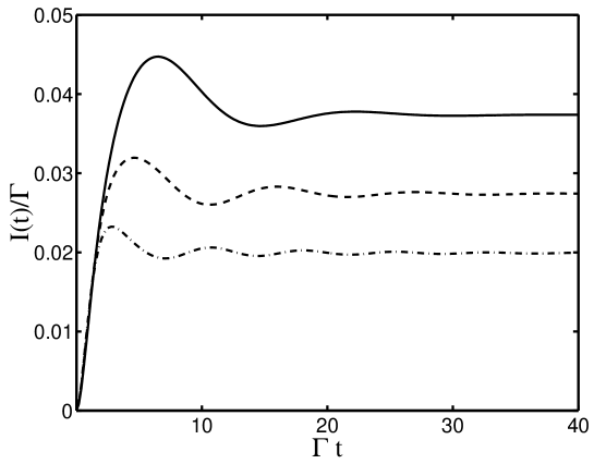
Figure 6: Time evolution of the total radiation intensity for the running-wave driving field with $\Omega=0.2\Gamma,\vec{k}_{L}\parallel\vec{r}_{12}$ and different interatomic separations; $r_{12}=0.2\lambda$ (solid line), $r_{12}=0.16\lambda$ (dashed line), $r_{12}=0.14\lambda$ (dashed-dotted line).

Figures 6 and 7 show the time evolution of the total radiation intensity, obtained by numerical solutions of the equations of motion for the atomic correlation functions. The equations are found from the master equation (42), which in the case of the running- or standing-wave driving field leads to a closed set of fifteen equations of motion for the atomic correlation functions [90, 91]. In Fig. 6, we present the time-dependent total radiation intensity for the running-wave driving field with $\Omega=0.2\Gamma,\vec{k}_{L}\parallel\vec{r}_{12}$ and different interatomic separations. Fig. 7 shows the total radiation intensity for the same parameters as in Fig. 6, but the standing-wave driving field. As predicted by Eqs. (119) and (120), the intensity exhibits quantum beats. The amplitude and frequency of the oscillations is dependent on the interatomic interactions and vanishes for large interatomic separations as well as for separations very small compared with the resonant wavelength. This is easily explained in the framework of collective states of a two-atom system. For a weak driving field, the population oscillates between the intermediate states $|{s}\rangle$, $|{a}\rangle$ and the ground state $|{g}\rangle$. When interatomic separations are large, $\Omega_{12}$ is approximately zero, and then the transitions $|{s}\rangle\rightarrow|{g}\rangle$ and $|{a}\rangle\rightarrow|{g}\rangle$ have the same frequency. Therefore, there are no quantum beats in the emitted field. On the other hand, for very small interatomic separations, $\vec{k}_{L}\cdot\vec{r}_{12}\approx 0$, and then the coupling parameters $\Gamma_{as}$ and $\Delta_{c}$ vanish, resulting in the disappearance of the quantum beats.

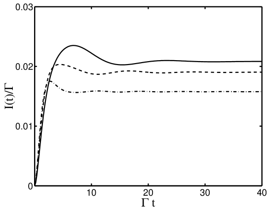
Figure 7: Time evolution of the total radiation intensity for the same parameters as in Fig. 6, but the standing-wave driving field.

5 Nonclassical states of light

The interaction of light with atomic systems can lead to unique phenomena such as photon antibunching and squeezing. These effects are examples of a nonclassical light field, that is a field for which quantum mechanics is essential for its description. Photon antibunching is characteristic of a radiation in which the variance of the number of photons is less than the mean number of photons, i.e. the photons exhibit sub-Poissonian statistics. Squeezing is characteristic of a field with phase-sensitive quantum fluctuations, which in one of the two phase components are reduced below the vacuum (shot-noise) level. Since photon antibunching and squeezing are distinguishing features of light, it is clearly of interest to identify situations in which such fields can be generated. Photon antibunching has been predicted theoretically for the first time in resonance fluorescence of a two-level atom [101, 102]. Since then, a number of papers have appeared analyzing various schemes for generating photon antibunching offered by nonlinear optics [103, 104, 105, 106]. Squeezing has been extensively studied since the theoretical work by Walls and Zoller [107] and Mandel [108] on reduction of noise and photon statistics in resonance fluorescence of a two-level atom. Several experimental groups have been successful in producing nonclassical light. Photon antibunching has been observed in resonance fluorescence from a dilute atomic beam of sodium atoms driven by a coherent laser field [109, 110, 111]. More recently, beautiful measurements of photon antibunching have been made on trapped atoms [112], and a cavity QED system [113]. On the other hand, squeezed light was first observed by Slusher et al. [114] in four-wave mixing experiments. After that observation squeezed light has been observed in many other nonlinear processes, with a recent development being the availability of a tunable source of squeezed light exhibiting a noise reduction of $\sim 70\%$ below the shot-noise level. The experimental observation of photon antibunching and squeezing have provided direct evidence of the quantum nature of light, and these two phenomena were precursors of much of the present work on nonclassical light fields. An extensive literature on various aspects of photon antibunching and squeezing now exists and is reviewed in several articles [115, 116, 117].

The objective of this section is to concentrate on collective two-atom systems as a potential source for photon antibunching and squeezing. We understand collective effects in a broad sense, that for two or more atoms all effects that cannot be explained by the properties of individual atoms are considered as collective. This definition of collective effects thus includes, for example, both the resonance fluorescence from a system of two atoms in free space and also collective behaviour of two atoms strongly coupled to the same cavity mode in the good cavity limit. Moreover, we emphasize the role of the interatomic interactions in the generation of nonclassical light. We also relate the nonclassical effects to the degree of entanglement in the system.

5.1 Photon antibunching

Photon antibunching is described through the normalized second-order correlation function, defined as [86]

$$g^{(2)}\left(\vec{R}_{1},t_{1};\vec{R}_{2},t_{2}\right)=\frac{G^{(2)}\left(\vec{R}_{1},t_{1};\vec{R}_{2},t_{2}\right)}{G^{(1)}\left(\vec{R}_{1},t_{1}\right)G^{(1)}\left(\vec{R}_{2},t_{2}\right)}\ ,$$ (121)

where

$$G^{(2)} \left(\vec{R}_{1},t_{1};\vec{R}_{2},t_{2}\right)$$ (122)

$$=\langle\vec{E}^{(-)}\left(\vec{R}_{1},t_{1}\right)\vec{E}^{(-)}\left(\vec{R}_{2},t_{2}\right)\vec{E}^{(+)}\left(\vec{R}_{2},t_{2}\right)\vec{E}^{(+)}\left(\vec{R}_{1},t_{1}\right)\rangle\ ,$$

is the two-time second-order correlation function of the EM field detected at a point $\vec{R}_{1}$ at time $t_{1}$ and at a point $\vec{R}_{2}$ at time $t_{2}$, and

$$G^{(1)}\left(\vec{R}_{i},t_{i}\right) = \langle\vec{E}^{(-)}\left(\vec{R}_{i},t_{i}\right)\vec{E}^{(+)}\left(\vec{R}_{i},t_{i}\right)\rangle\ ,$$ (123)

is the first-order correlation function of the field (intensity) detected at a point $R_{i}$ at time $t_{i}(i=1,2)$.

The correlation function $G^{(2)}(\vec{R}_{1},t_{1};\vec{R}_{2},t_{2})$ is proportional to a joint probability of finding one photon around the direction $\vec{R}_{1}$ at time $t_{1}$ and another photon around the direction $\vec{R}_{2}$ at the moment of time $t_{2}$. For a coherent light, the probability of finding a photon around $\vec{R}_{1}$ at time $t_{1}$ is independent of the probability of finding another photon around $\vec{R}_{2}$ at time $t_{2}$, and then $G^{(2)}(\vec{R}_{1},t_{1};\vec{R}_{2},t_{2})$ simply factorizes into $G^{(1)}(\vec{R}_{1},t_{1})G^{(1)}(\vec{R}_{2},t_{2})$ giving $g^{(2)}(\vec{R}_{1},t_{1};\vec{R}_{2},t_{2})=1$. For a chaotic (thermal) field the second-order correlation function for $t_{1}=t_{2}$ is greater than for $t_{2}-t_{1}=\tau>0$ giving $g^{(2)}(\vec{R}_{1},t_{1};\vec{R}_{2},t_{1})>g^{(2)}(\vec{R}_{1},t_{1};\vec{R}_{2},t_{1}+\tau)$. This is a manifestation of the tendency of photons to be emitted in correlated pairs, and is called photon bunching. Photon antibunching, as the name implies, is the opposite of bunching, and describes a situation in which fewer photons appear close together than further apart. The condition for photon antibunching is $g^{(2)}(\vec{R}_{1},t_{1};\vec{R}_{2},t_{1})<g^{(2)}(\vec{R}_{1},t_{1};\vec{R}_{2},t_{1}+\tau)$ and implies that the probability of detecting two photons at the same time $t$ is smaller than the probability of detecting two photons at different times $t$ and $t+\tau$. Moreover, the fact that there is a small probability of detecting photon pairs with zero time separation indicated that the one-time correlation function $g^{(2)}(\vec{R}_{1},t;\vec{R}_{2},t)$ is smaller than one. This effect is called photon anticorrelation. The normalized one-time second-order correlation function carries also information about photon statistics, which is given by the Mandel’s $Q$ parameter defined as [108]

$$Q=qT\left[g^{(2)}\left(\vec{R}_{1},t;\vec{R}_{2},t\right)-1\right]\ ,$$ (124)

where $q$ is the quantum efficiency of the detector and $T$ is the photon counting time.

We can relate the field correlation functions (122) and (123) to the correlation functions of the atomic operators, which will allow us to apply directly the master equation (42) to calculate photon antibunching in a collective atomic system. The relation between the positive frequency part of the electric field operator at a point $\vec{R}=R\bar{R}$, in the far-field zone, and the atomic dipole operators $S_{i}^{-}$, is given by the well-known expression [47, 49]

$$\vec{E}^{(+)}\left(\vec{R},t\right) = \vec{E}^{(+)}_{0}\left(\vec{R},t\right)$$ (125)

$$- \sum_{i=1}^{2}\frac{\omega_{i}}{c^{2}}\frac{\bar{R}\times\left(\bar{R}\times\vec{\mu}_{i}\right)}{R}S_{i}^{-}\left(t-\frac{R}{c}\right)\exp\left(-ik\bar{R}\cdot\vec{r}_{i}\right)\ ,$$

where $\omega_{i}$ is the angular frequency of the $i$th atom located at a point $\vec{r}_{i}$, and $\vec{E}^{(+)}_{0}\left(\vec{R},t\right)$ denotes the positive frequency part of the field in the absence of the atoms.

If we assume that initially the field is in the vacuum state, then the free-field part $\vec{E}^{(+)}_{0}(\vec{R},t)$ does not contribute to the expectation values of the normally ordered operators. Hence, substituting Eq. (125) into Eqs. (122) and (123), we obtain

$$G^{\left(2\right)}\left(\vec{R},t;\vec{R},t+\tau\right) = u(\vec{R}_{1})u(\vec{R}_{2})\sum_{i,j,k,l=1}^{N}\left(\Gamma_{i}\Gamma_{j}\Gamma_{k}\Gamma_{l}\right)^{\frac{1}{2}}$$ (126)

$$\times \left\langle S^{+}_{i}\left(t\right)S^{+}_{k}\left(t+\tau\right)S^{-}_{l}\left(t+\tau\right)S^{-}_{j}\left(t\right)\right\rangle$$

$$\times \exp\left[ik\left(\bar{R}_{1}\cdot\vec{r}_{ij}+\bar{R}_{2}\cdot\vec{r}_{kl}\right)\right]\ ,$$

$$G^{\left(1\right)}\left(\vec{R},t\right) = u(\vec{R})\sum_{i,j=1}^{N}\left(\Gamma_{i}\Gamma_{j}\right)^{\frac{1}{2}}\left\langle S_{i}^{+}\left(t\right)S^{-}_{j}\left(t\right)\right\rangle$$ (127)

$$\times \exp\left(ik\bar{R}\cdot\vec{r}_{ij}\right)\ ,$$

where $\tau=t_{2}-t_{1}$, $\Gamma_{i}$ is the damping rate of the $i$th atom, and $u(\vec{R})$ is a constant given in Eq. (74). The second-order correlation function (126) involves two-time atomic correlation function that can be calculated from the master equation (36) or (42) and applying the quantum regression theorem [118]. From the quantum regression theorem, it is well known that for $\tau>0$ the two-time correlation function $\langle S^{+}_{i}\left(t\right)S^{+}_{k}\left(t+\tau\right)S^{-}_{l}\left(t+\tau\right)S^{-}_{j}\left(t\right)\rangle$ satisfies the same equation of motion as the one-time correlation function $\langle S_{k}^{+}\left(t\right)S^{-}_{l}\left(t\right)\rangle$.

We shall first of all consider the simplest collective system for photon antibunching; two identical atoms in the Dicke model. Whilst this model is not well satisfied with the present sources of two-atom systems, it does enable analytic treatments that allow to understand the role of the collective damping in the generation of nonclassical light.

For the two-atom Dicke model the master equation (42) reduces to

$$\frac{\partial\hat{\rho}}{\partial t} = \frac{1}{2}i\Omega\left[S^{+}+S^{-},\hat{\rho}\right]-\frac{1}{2}\Gamma\left(S^{+}S^{-}\hat{\rho}+\hat{\rho}S^{+}S^{-}-2S^{-}\hat{\rho}S^{+}\right)\ ,$$ (128)

where $S^{\pm}=S^{\pm}_{1}+S^{\pm}_{2}$ and $S^{z}=S^{z}_{1}+S^{z}_{2}$ are the collective atomic operators and $\Omega$ is the Rabi frequency of the driving field, which in the Dicke model is the same for both atoms. For simplicity, the laser frequency $\omega_{L}$ is taken to be exactly equal to the atomic resonant frequency $\omega_{0}$.

The secular approximation technique has been suggested by Agarwal et al. [119] and Kilin [120], which greatly simplifies the master equation (128). Hassan et al. [121] and Cordes [122, 123] have generalised the method to include non-zero detuning of the laser field and the quasistatic dipole-dipole potential. The technique is a modification of a collective dressed-atom approach developed by Freedhoff [124] and is valid if the Rabi frequency of the driving field is much greater than the damping rates of the atoms, $\Omega\gg\Gamma$. To implement the technique, we transform the collective operators into new (dressed) operators

$$S^{\pm} = \pm\frac{1}{2}i\left(R^{+}+R^{-}\right)+R^{z}\ ,$$

$$S^{z} = -\frac{1}{2}i\left(R^{+}-R^{-}\right)\ .$$ (129)

The operators $R$ are a rotation of the operators $S$. For a strong driving field, the operators $R^{\pm}$ vary rapidly with time, approximately as $\exp(\pm i\Omega t)$, while $R^{z}$ varies slowly in time. By expressing the operators $S^{\pm}$ and $S^{z}$ in terms of the operators $R^{\pm}$ and $R^{z}$, and substituting into the master equation (128), we find that certain terms are slowly varying in time while others oscillate rapidly. The secular approximation then involves dropping the rapidly oscillating terms that results in an approximate master equation of the form

$$\frac{\partial\hat{\rho}}{\partial t}=i\Omega\left[R^{z},\hat{\rho}\right] - \frac{1}{2}\Gamma\left\{\left(R^{z}R^{z}\hat{\rho}+\hat{\rho}R^{z}R^{z}-2R^{z}\hat{\rho}R^{z}\right)\right.$$ (130)

$$\left.+\frac{1}{4}\left(R^{+}R^{-}\hat{\rho}+\hat{\rho}R^{+}R^{-}-2R^{-}\hat{\rho}R^{+}\right)\right.$$

$$\left.+\frac{1}{4}\left(R^{-}R^{+}\hat{\rho}+\hat{\rho}R^{-}R^{+}-2R^{+}\hat{\rho}R^{-}\right)\right\}\ .$$

The master equation (130) enables to obtain equations of motion for the expectation value of an arbitrary combination of the transformed operators $R$. In particular, the master equation leads to simple equations of motion for the expectation values required to calculate the normalized second-order correlation function. The required equations of motion are given by

$$\frac{d}{dt}\left\langle R^{z}\right\rangle = -\frac{1}{2}\Gamma\left\langle R^{z}\right\rangle\ ,$$

$$\frac{d}{dt}\langle R^{\pm}\rangle = -\left(\frac{3}{4}\Gamma\pm i\Omega\right)\langle R^{\pm}\rangle\ ,$$

$$\frac{d}{dt}\langle R^{+}R^{+}\rangle = -\left(\frac{5}{2}\Gamma+2i\Omega\right)\langle R^{+}R^{+}\rangle\ .$$ (131)

The solution of these decoupled differential equations is straightforward. Performing the integration and applying the quantum regression theorem [118], we obtain from Eqs. (131) and (121) the following solution for the normalized second-order correlation function [84, 125]

$$g^{(2)}\left(\tau\right) \equiv \lim_{t\rightarrow\infty}g^{(2)}\left(\vec{R}_{1},t;\vec{R}_{2},t+\tau\right)=1+\frac{1}{32}\exp\left(-\frac{3}{2}\Gamma\tau\right)$$ (132)

$$+\frac{3}{32}\exp\left(-\frac{5}{2}\Gamma\tau\right)\cos\left(2\Omega\tau\right)-\frac{3}{8}\exp\left(-\frac{3}{4}\Gamma\tau\right)\cos\left(\Omega\tau\right)\ .$$

The correlation function $g^{(2)}\left(\tau\right)$ is shown in Fig. 8 as a function of $\tau$ for different $\Omega$. For $\tau=0$, the correlation function $g^{(2)}\left(0\right)=0.75$, showing the photon anticorrelation in the emitted fluorescence field. As $\tau$ increases, the correlation function increases $(g^{(2)}\left(\tau\right)>g^{(2)}\left(0\right))$, which reflects photon antibunching in the emitted field. However, the photon anticorrelation in the two-atom fluorescence field is reduced compared to that for a single atom, for which $g^{(2)}\left(0\right)=0$. This result indicates that the collective damping reduces the photon anticorrelations in the emitted fluorescence field.

Figure 8: The normalised second-order correlation function $g^{(2)}\left(\tau\right)$ as a function of $\tau$ and different $\Omega$; $\Omega=2.5\Gamma$ (solid line), $\Omega=10\Gamma$ (dashed line).

As we have mentioned above, in the Dicke model the dipole-dipole interaction between the atoms is ignored. This approximation has no justification, since for small interatomic separations the dipole-dipole parameter $\Omega_{12}$, which varies as $(k_{0}r_{12})^{-3}$, is very large and goes to infinity as $r_{12}$ goes to zero (see Fig. 1). Moreover, the Dicke model does not correspond to the experimentally realistic systems in which atoms are separated by distances comparable to the resonant wavelength. Ficek et al. [84] and Lawande et al. [126] have shown that the dipole-dipole interaction does not considerably affect the anticorrelation effect predicted in the Dicke model. Richter [127] has shown that the value $g^{(2)}\left(0\right)=0.75$ can in fact be reduced such that even the complete photon anticorrelation $g^{(2)}\left(0\right)=0$ can be obtained, if the dipole-dipole is included and the laser frequency is detuned from the atomic transition frequency. To show this, we calculate the normalized second-order correlation function (121) for the steady-state fluorescence field from two identical atoms $(N=2)$, and $\tau=0$. In this case, the correlation function (121) with Eqs. (126) and (127) can be written as

$$g^{(2)}\left(0\right)=\frac{2U\left\{1+\cos\left[k\vec{r}_{12}\cdot\left(\bar{R}_{1}-\bar{R}_{2}\right)\right]\right\}}{\left[1+W\cos\left(k\vec{r}_{12}\cdot\bar{R}_{1}\right)\right]\left[1+W\cos\left(k\vec{r}_{12}\cdot\bar{R}_{2}\right)\right]}\ ,$$ (133)

where $U$ and $W$ are the steady-state atomic correlation functions

$$U=\frac{\langle S^{+}_{1}S^{+}_{2}S^{-}_{1}S^{-}_{2}\rangle}{\langle S^{+}_{1}S^{-}_{1}+S^{+}_{2}S^{-}_{2}\rangle^{2}}\ ,\qquad W=\frac{\langle S^{+}_{1}S^{-}_{2}+S^{+}_{2}S^{-}_{1}\rangle}{\langle S^{+}_{1}S^{-}_{1}+S^{+}_{2}S^{-}_{2}\rangle}\ .$$ (134)

The steady-state correlation functions are easily obtained from the master equation (42). We can simplify the solutions assuming that the atoms are in equivalent positions in the driving field, which can be achieved by propagating the laser field in the direction perpendicular to the interatomic axis. In this case we get analytical solutions, otherwise for $\vec{k}_{L}\cdot\vec{r}_{12}\neq 0$ numerical methods are more appropriate [90, 91, 128]. With $\vec{k}_{L}\cdot\vec{r}_{12}=0$ the master equation (42) leads to a closed set of nine equations of motion for the atomic correlation functions. This set of equations can be solved exactly in the steady-state [129], and the solutions for $U$ and $W$ are

$$U = \frac{\Omega^{4}+\left(\Gamma^{2}+4\Delta_{L}^{2}\right)\Omega^{2}+\left(\Gamma^{2}+4\Delta_{L}^{2}\right)\left[\frac{1}{4}\left(\Gamma+\Gamma_{12}\right)^{2}+\left(\Delta_{L}-\Omega_{12}\right)^{2}\right]}{\left(\Gamma^{2}+4\Delta_{L}^{2}+2\Omega^{2}\right)^{2}}\ ,$$

$$W = \frac{\left(\Gamma^{2}+4\Delta_{L}^{2}\right)}{\left(\Gamma^{2}+4\Delta_{L}^{2}+2\Omega^{2}\right)}\ .$$ (135)

One can see from Eqs. (133) and (135) that there are two different processes which can lead to the total anticorrelation, $g^{(2)}\left(0\right)=0$. The first one involves an observation of the fluorescence field with two detectors located at different points. If the correlation function is measured using two detectors, $\bar{R}_{1}\neq\bar{R}_{2}$, and then we obtain $g^{(2)}\left(0\right)=0$ whenever the positions of the detectors are such that

$$\left\{1+\cos\left[k\vec{r}_{12}\cdot\left(\bar{R}_{1}-\bar{R}_{2}\right)\right]\right\}=0\ ,$$ (136)

which happens when

$$k\vec{r}_{12}\cdot\left(\bar{R}_{1}-\bar{R}_{2}\right)=\left(2n+1\right)\pi\ ,\quad n=0,\pm 1,\pm 2\ldots$$ (137)

In other words, two photons can never be simultaneously detected at two points separated by an odd number of $\lambda/2r_{12}$, despite the fact that one photon can be detected anywhere. This complete anticorrelation effect is due to spatial interference between different photons and reflects the fact that one photon must have come from one source and one from the other, but we cannot tell which came from which.

It should be emphasised that this effect is independent of the interatomic interactions and the Rabi frequency of the driving field. The vanishing of $g^{(2)}\left(0\right)$ for two photons at widely separated points $\vec{R}_{1}$ and $\vec{R}_{2}$ is an example of quantum-mechanical nonlocality, that the outcome of a detection measurement at $\vec{R}_{1}$ appears to be influenced by where we have chosen to locate the $\vec{R}_{2}$ detector. At certain positions $\vec{R}_{2}$ we can never detect a photon at $\vec{R}_{1}$ when there is a photon detected at $\vec{R}_{2}$, whereas at other position $\vec{R}_{2}$ it is possible. The photon correlation argument shows clearly that quantum theory does not in general describe an objective physical reality independent of observation.

The second process involves the shift of the collective atomic states due to the dipole-dipole interaction that can lead to $g^{(2)}\left(0\right)=0$ even if the correlation function is measured with a single detector $(\bar{R}_{1}=\bar{R}_{2})$ or two detectors in configurations different from that given by Eq. (137). For a weak driving field $(\Omega\ll\Gamma)$ and large detunings such that $\Delta_{L}=\Omega_{12}\gg\Gamma$, the correlation function (121) with $\bar{R}_{1}=\bar{R}_{2}$ simplifies to

$$g^{(2)}\left(0\right)\approx\frac{\left(\Gamma+\Gamma_{12}\right)^{2}}{4\Delta_{L}^{2}}\ .$$ (138)

Figure 9: The normalised second-order correlation function $g^{(2)}\left(0\right)$ as a function of $\Delta_{L}$ for $\bar{R}_{1}=\bar{R}_{2}=\bar{R},\vec{r}_{12}\perp\bar{R},\bar{\mu}\perp\bar{r}_{12}$, $\Omega=0.5\Gamma$ and different $r_{12}$; $r_{12}=10\lambda$ (solid line), $r_{12}=0.15\lambda$ (dashed line), $r_{12}=0.08\lambda$ (dashed-dotted line).

Thus, a pronounced photon anticorrelation, $g^{(2)}\left(0\right)\approx 0$, can be obtained for large detunings such that $\Delta_{L}=\Omega_{12}$, i.e., when the dipole-dipole interaction shift of the collective states and the detuning cancel out mutually. The correlation function $g^{(2)}\left(0\right)$ of the steady-state fluorescence field is illustrated graphically in Fig. 9 as a function of $\Delta_{L}$ for the single detector configuration with $\bar{R}_{1}=\bar{R}_{2}=\bar{R}$, and different $r_{12}$. The graphs show that $g^{(2)}\left(0\right)$ strongly depends on $\Delta_{L}$, and the total photon anticorrelation can be obtained for $\Delta_{L}=\Omega_{12}$. Referring to Fig. 2, the condition $\Delta_{L}=\Omega_{12}$ corresponds to the laser frequency tuned to the resonance with the $|{g}\rangle\rightarrow|{s}\rangle$ transition. Since the other levels are far from the resonance, the two-atom system behaves like a single two-level system with the ground state $|{g}\rangle$ and the excited state $|{s}\rangle$.

5.2 Squeezing

To understand squeezed light, recall that the electric field amplitude $\vec{E}\left(\vec{r}\right)$ may be expressed by positive- and negative-frequency parts

$$\vec{E}\left(\vec{r}\right)=\vec{E}^{\left(+\right)}\left(\vec{r}\right)+\vec{E}^{\left(-\right)}\left(\vec{r}\right)\ ,$$ (139)

where

$$\vec{E}^{\left(+\right)}\left(\vec{r}\right)=\left(\vec{E}^{\left(-\right)}\left(\vec{r}\right)\right)^{\dagger}=-i\sum_{\vec{k}s}\left(\hbar\omega_{k}/2\varepsilon_{o}V\right)^{1/2}\bar{e}_{\vec{k}s}\hat{a}_{\vec{k}s}e^{i\vec{k}\cdot\vec{r}}\ ,$$ (140)

and $\omega_{k}=c\left|\vec{k}\right|$ is the angular frequency of the mode $\vec{k}$.

We introduce two Hermitian combinations (quadrature components) of the field components that are $\pi/2$ out of phase as

$$\vec{E}_{\theta} = \vec{E}^{\left(+\right)}\left(\vec{R}\right)e^{i\theta}+\vec{E}^{\left(-\right)}\left(\vec{R}\right)e^{-i\theta}\ ,$$

$$\vec{E}_{\theta-\pi/2} = -i\left(\vec{E}^{\left(+\right)}\left(\vec{R}\right)e^{i\theta}-\vec{E}^{\left(-\right)}\left(\vec{R}\right)e^{-i\theta}\right)\ ,$$ (141)

where

$$\theta=\omega t-\vec{k}\cdot\vec{R}\ ,$$ (142)

and $\omega$ is the angular frequency of the quadrature components.

The quadrature components do not commute, satisfying the commutation relation

$$\left[\vec{E}_{\theta},\vec{E}_{\theta-\pi/2}\right]=2iC\ ,$$ (143)

where $C$ is a positive number

$$C=\sum_{\vec{k}s}\left|\hbar\omega_{k}/2\varepsilon_{o}V\right|\ .$$ (144)

Hence the two quadrature components cannot be simultaneously precisely measured, and from the Heisenberg uncertainty principle, we find that the variances $\left\langle\Delta\vec{E}_{\theta}^{2}\right\rangle$ and $\left\langle\Delta\vec{E}_{\theta-\pi/2}^{2}\right\rangle$ satisfy the inequality

$$\left\langle\Delta\vec{E}_{\theta}^{2}\right\rangle\left\langle\Delta\vec{E}_{\theta-\pi/2}^{2}\right\rangle\geq C^{2}\ ,$$ (145)

where the equality holds for a minimum uncertainty state of the field.

The variances $\left\langle\Delta\vec{E}_{\theta}^{2}\right\rangle$ and $\left\langle\Delta\vec{E}_{\theta-\pi/2}^{2}\right\rangle$ depend on the state of the field and can be larger or smaller than $C$. A chaotic state of the field leads to the variances in both components larger than $C$:

$$\left\langle\Delta\vec{E}_{\theta}^{2}\right\rangle\geq C\quad \quad\left\langle\Delta\vec{E}_{\theta-\pi/2}^{2}\right\rangle\geq C\ .$$ and (146)

If the field is in a coherent or vacuum state

$$\left\langle\Delta\vec{E}_{\theta}^{2}\right\rangle=\left\langle\Delta\vec{E}_{\theta-\pi/2}^{2}\right\rangle=C\ ,$$ (147)

which is an example of a minimum uncertainty state.

A squeezed state of the field is defined to be one in which the variance in one of the two quadrature components is less than that for the vacuum field

$$\left\langle\Delta\vec{E}_{\theta}^{2}\right\rangle<C\quad \quad\left\langle\Delta\vec{E}_{\theta-\pi/2}^{2}\right\rangle<C\ .$$ or (148)

The variances can be expressed as

$$\left\langle\Delta\vec{E}_{\theta}^{2}\right\rangle = C+\left\langle:\Delta\vec{E}_{\theta}^{2}:\right\rangle\ ,$$

$$\left\langle\Delta\vec{E}_{\theta-\pi/2}^{2}\right\rangle = C+\left\langle:\Delta\vec{E}_{\theta-\pi/2}^{2}:\right\rangle\ ,$$ (149)

where the colon stands for normal ordering of the operators.

As the squeezed state has been defined by the requirement that either $\left\langle\Delta\vec{E}_{\theta}^{2}\right\rangle$ or $\left\langle\Delta\vec{E}_{\theta-\pi/2}^{2}\right\rangle$ be below the vacuum level $C$, it follows immediately from Eq. (149) that either

$$\left\langle:\Delta\vec{E}_{\theta}^{2}:\right\rangle<0\quad \quad\left\langle:\Delta\vec{E}_{\theta-\pi/2}^{2}:\right\rangle<0$$ or (150)

for the field in a squeezed state.

We now determine the relation between variances in the field and the atomic dipole operators. Using Eq. (125), which relates the field operators to the atomic dipole operators, we obtain

$$\left\langle:\Delta\vec{E}_{\alpha}^{2}:\right\rangle=u\left(\vec{R}\right)\left[\langle\left(\Delta S_{\alpha}\right)^{2}\rangle+\frac{1}{2}\langle S_{3}\rangle\right]\ ,$$ (151)

where $\alpha=\theta,\theta-\pi/2$, $S_{\alpha}$ and $S_{3}$ are real (phase) operators defined as

$$S_{\theta} = \frac{1}{2}\left(S_{\theta}^{+}+S_{\theta}^{-}\right)\ ,\qquad S_{\theta-\pi/2}=\frac{1}{2i}\left(S_{\theta}^{+}-S_{\theta}^{-}\right)\ ,$$ (152)

and

$$S_{3}=\frac{1}{2}\left[S_{\theta}^{+},S_{\theta}^{-}\right]\ ,$$ (153)

with

$$S_{\theta}^{\pm}=\sum_{i=1}^{N}S_{i}^{\pm}\exp\left[\pm i\left(k\bar{R}\cdot\vec{r}_{i}-\theta\right)\right]\ .$$ (154)

We first consider quantum fluctuations in the fluorescence field emitted by two identical atoms in the Dicke model. To simplify the calculations we will treat only the case of zero detuning, $\Delta_{L}=0$. Assuming that initially $(t=0)$ the atoms were in their ground states, we find from Eqs. (131) and (151) the following expressions for the time-dependent variances [130]

$$F_{\theta=0}\left(t\right) \equiv \left\langle:\Delta\vec{E}_{\theta=0}^{2}:\right\rangle/\left(2u(\vec{R})\right)=\frac{1}{3}-\frac{1}{8}\exp\left(-\frac{5}{2}\Gamma t\right)\cos\left(2\Omega t\right)$$ (155)

$$+ \frac{1}{24}\exp\left(-\frac{3}{2}\Gamma t\right)-\frac{1}{2}\exp\left(-\frac{3}{2}\Gamma t\right)\sin^{2}\left(\Omega t\right)$$

$$- \frac{1}{4}\exp\left(-\frac{3}{4}\Gamma t\right)\cos\left(\Omega t\right)\ ,$$

and

$$F_{\theta=\pi/2}\left(t\right) \equiv \left\langle:\Delta\vec{E}_{\theta=\pi/2}^{2}:\right\rangle/\left(2u(\vec{R})\right)=\frac{1}{3}-\frac{1}{12}\exp\left(-\frac{3}{2}\Gamma t\right)$$ (156)

$$- \frac{1}{4}\exp\left(-\frac{3}{4}\Gamma t\right)\cos\left(\Omega t\right)\ .$$

In writing Eqs. (155) and (156), we have assumed that the angular frequency of the quadrature components is equal to the laser frequency, $\omega=\omega_{L}$, and we have normalised the variances such that $F(t)$ determines fluctuations per atom. It is easily to show that the variance $F_{\theta=\pi/2}\left(t\right)$ is positive for all times $t$, and squeezing $(F_{\theta}<0)$ can be observed in the variance $F_{\theta=0}\left(t\right)$. The time dependence of the variance $F_{\theta=0}\left(t\right)$ is shown in Fig. 10 for two different values of the Rabi frequency. It is seen that squeezing appears in the transient regime of resonance fluorescence and its maximum value (minimum of $F$) moves towards shorter times as $\Omega$ increases. The optimum squeezing reaches a value of $-1/16$ at a very short time. This value is equal to the maximum possible squeezing in a single two-level atom [107, 131, 132, 133]. Thus, the collective damping does not affect squeezing in the two-atom Dicke model. This is in contrast to the photon anticorrelation effect which is greatly reduced by the collective damping.

Figure 10: The variance $F_{\theta=0}\left(t\right)$ as a function of time for different $\Omega$; $\Omega=100\Gamma$ (solid line), $\Omega=200\Gamma$ (dashed line).

Figure 10 shows that in the two-atom Dicke model there is no squeezing in the steady-state resonance fluorescence when the atoms are excited by a strong laser field. Ficek et al. [129] and Richter [134] have shown that similarly as in the case of photon anticorrelations, a large squeezing can be obtained in the steady-state resonance fluorescence from a strongly driven two-atom system, if the dipole-dipole interaction is included and the laser frequency is detuned from the atomic transition frequency. This is shown in Fig. 11, where we plot $F_{\theta=0}$, calculated from Eq. (151) and the master equation (42), for the steady-state resonance fluorescence from two identical atoms, with $\vec{r}_{12}\perp\bar{R}$, $\Omega=0.5\Gamma$, $\vec{k}_{L}\cdot\vec{r}_{12}=0$ and different $r_{12}$. It is evident from Fig. 11 that a large squeezing can be obtained for a finite $\Delta_{L}$ and its maximum shifts towards larger $\Delta_{L}$ as the interatomic separation decreases. Similar as in the case of photon anticorrelations, the maximum squeezing appears at $\Delta_{L}=\Omega_{12}$, and can again be attributed to the shift of the collective energy states due to the dipole-dipole interaction.

The variance $F_{\theta=0}$, shown in Fig. 11, exhibits not only the large squeezing at finite detuning $\Delta_{L}$, but also a small squeezing near $\Delta_{L}=0$. In contrast to the squeezing at finite $\Delta_{L}$, which has a clear physical interpretation, the source of squeezing at $\Delta_{L}$ is not easy to understand. To find the source of squeezing at $\Delta_{L}=0$, we simplify the calculations assuming that the angular frequency of the quadrature components $\omega=\omega_{L}$ and the fluorescence field is observed in the direction perpendicular to the interatomic axis, $\bar{R}\perp\vec{r}_{12}$. In this case, the variance $\left\langle:\Delta\vec{E}_{\alpha}^{2}:\right\rangle$, written in terms of the density matrix elements of the collective system, is given by [135]

$$F_{\alpha}\equiv\left\langle:\Delta\vec{E}_{\alpha}^{2}:\right\rangle/\left(2u(\vec{R})\right) = \frac{1}{4}\left\{2\rho_{ee}+2\rho_{ss}+\rho_{eg}e^{2i\alpha}+\rho_{ge}e^{-2i\alpha}\right.$$ (157)

$$- \left.\left[\left(\rho_{es}+\rho_{sg}\right)e^{i\alpha}+\left(\rho_{se}+\rho_{gs}\right)e^{-i\alpha}\right]^{2}\right\}\ .$$

This equation shows that the variance depends on phase $\alpha$ not only through the one-photon coherences $\rho_{es}$ and $\rho_{sg}$, but also through the two-photon coherences $\rho_{eg}$ and $\rho_{ge}$. This dependence suggests that there are two different processes that can lead to squeezing in the two-atom system. The one-photon coherences cause squeezing near one-photon resonances $|{e}\rangle\rightarrow|{s}\rangle$ and $|{s}\rangle\rightarrow|{g}\rangle$, whereas the two-photon coherences cause squeezing near the two-photon resonance $|{g}\rangle\rightarrow|{e}\rangle$.

Figure 11: The steady-state variance $F_{\theta=0}$ as a function of $\Delta_{L}$ for $\vec{r}_{12}\perp\bar{R}$, $\bar{\mu}\perp\bar{r}_{12}$, $\Omega=0.5\Gamma$, $\vec{k}_{L}\cdot\vec{r}_{12}=0$ and different $r_{12}$; $r_{12}=10\lambda$ (solid line), $r_{12}=0.15\lambda$ (dashed line), $r_{12}=0.08\lambda$ (dashed-dotted line).

To show this, we calculate the steady-state populations and coherences from the master equation (42). We use the set of the collective states (67) as an appropriate representation for the density operator

$$\hat{\rho}=\sum_{ij}\rho_{ij}|{i}\rangle\langle{j}|,\quad i,j=g,s,a,e\ ,$$ (158)

where $\rho_{ij}$ are the density matrix elements in the basis of the collective states.

After transforming to the collective state basis, the master equation (42) leads to a closed system of fifteen equations of motion for the density matrix elements [84]. However, for a specifically chosen geometry for the driving field, namely that the field is propagated perpendicularly to the atomic axis $(\vec{k}_{L}\cdot\vec{r}_{12}=0)$, the system of equations decouples into nine equations for symmetric and six equations for antisymmetric combinations of the density matrix elements [84, 85, 90, 91, 127, 128]. In this case, we can solve the system analytically, and find that the steady-state values of the populations and coherences are [84, 127]

$$\rho_{ee} = \rho_{aa}=\frac{\tilde{\Omega}^{4}}{Z}\ ,\qquad\rho_{ss}=\frac{\tilde{\Omega}^{2}\left(\Gamma^{2}+4\Delta^{2}_{L}\right)+\tilde{\Omega}^{4}}{Z}\ ,$$

$$\rho_{es} = i\tilde{\Omega}^{3}\left(\Gamma+2i\Delta_{L}\right)/Z\ ,$$

$$\rho_{sg} = -i\tilde{\Omega}\left\{\Gamma\tilde{\Omega}\left(\tilde{\Omega}+2i\Delta_{L}\right)\right.$$

$$\left.+\left(\Gamma^{2}+4\Delta_{L}^{2}\right)\left[\frac{1}{2}\left(\Gamma+\Gamma_{12}\right)+i\left(\Delta_{L}-\Omega_{12}\right)\right]\right\}/Z\ ,$$

$$\rho_{eg} = \tilde{\Omega}^{2}\left(\Gamma+2i\Delta_{L}\right)\left[\frac{1}{2}\left(\Gamma+\Gamma_{12}\right)+i\left(\Delta_{L}-\Omega_{12}\right)\right]/Z\ ,$$ (159)

where

$$Z=4\tilde{\Omega}^{4}+\left(\Gamma^{2}+4\Delta^{2}_{L}\right)\left\{2\tilde{\Omega}^{2}+\left[\frac{1}{4}\left(\Gamma+\Gamma_{12}\right)^{2}+\left(\Delta_{L}-\Omega_{12}\right)^{2}\right]\right\}\ ,$$ (160)

and $\tilde{\Omega}=\Omega/\sqrt{2}$.

Near the one-photon resonance $|{s}\rangle\rightarrow|{g}\rangle$ the detuning $\Delta_{L}=\Omega_{12}$, and assuming that $\Omega_{12}\gg\Omega,\Gamma$, the coherences reduce to

$$\rho_{es} = \frac{\tilde{\Omega}}{8\Omega_{12}}\ ,\qquad\rho_{sg}=\frac{-i\left(\Gamma+\Gamma_{12}\right)}{4\tilde{\Omega}}\ ,\qquad\rho_{eg}=\frac{i\left(\Gamma+\Gamma_{12}\right)}{8\Omega_{12}}\ .$$ (161)

It is clear from Eq. (161) that near the $|{g}\rangle\rightarrow|{s}\rangle$ resonance the coherence $\rho_{sg}$ is large, whereas the two-photon coherence is of order of $\Omega^{-1}_{12}$ and thus is negligible for large $\Omega_{12}$.

Near two-photon resonance, $\Delta_{L}\approx 0$, and it follows from Eq. (159) that in the limit of $\Omega_{12}\gg\Omega,\Gamma$ the coherences reduce to

$$\rho_{es}=\frac{i\tilde{\Omega}^{3}}{\Gamma\Omega_{12}^{2}}\ ,\qquad\rho_{sg}=-\frac{\tilde{\Omega}}{\Omega_{12}}\ ,\qquad\rho_{eg}=-\frac{i\tilde{\Omega}^{2}}{\Gamma\Omega_{12}}\ .$$ (162)

In this regime, the coherences $\rho_{sg}$ and $\rho_{eg}$ are of order of magnitude $\Omega^{-1}_{12}$, but $\rho_{eg}$ dominates over the one-photon coherence $\rho_{sg}$ when the driving field is strong [136].

Figure 12: The steady-state variance $F_{\alpha}$ as a function of $\Delta_{L}$ for $r_{12}=0.05\lambda$, $\Omega=3\Gamma$, $\bar{R}\perp\vec{r}_{12}$, $\bar{\mu}\perp\bar{r}_{12}$ and different phases $\alpha$: $\alpha=\pi/2$ (dashed line), $\alpha=3\pi/4$ (solid line).

The steady-state variance $F_{\alpha}$, calculated from Eqs. (157) and (159), is plotted in Fig. 12 as a function of $\Delta_{L}$ for $r_{12}=0.05\lambda$, $\Omega=3\Gamma$, $\bar{R}\perp\vec{r}_{12}$ and different phases $\alpha$. The variance shows a strong dependence on $\alpha$ near the one- and two-photon resonances. Moreover, a large squeezing is found at these resonances. It is also seen that near the two-photon resonance a change by $\pi/4$ of the phase $\alpha$ changes a dispersion-like structure of $F_{\alpha}$ into an absorption-like type. According to Eqs. (157) and (159), the variance $F_{\alpha}$ for $\Omega_{12}\gg\Omega\gg\Gamma$, can be written as

$$F_{\alpha}=\frac{\Omega^{2}}{\Omega_{12}}\left[\frac{\Delta_{L}}{\left(\Gamma^{2}+4\Delta_{L}^{2}\right)}\cos 2\alpha+\frac{\Gamma}{\left(\Gamma^{2}+4\Delta_{L}^{2}\right)}\sin 2\alpha\right]\ ,$$ (163)

where we retained only those terms which contribute near the two-photon resonance. Equation (163) predicts a dispersion-like structure for $\alpha=0$ or $\pi/2$, and an absorption-like structure for $\alpha=\pi/4$. Moreover, we see that the presence of the dipole-dipole interaction is essential to obtain squeezing near the two-photon resonance. The emergence of an additional dipole-dipole interaction induced squeezing is a clear indication of a totally different process which can appear in a two-atom system. The dipole-dipole interaction shifts the collective states that induces two-photon transitions responsible for the origin of the two-photon coherence.

6 Quantum interference of optical fields

In the classical theory of optical interference the EM field is represented by complex vectorial amplitudes $\vec{E}(\vec{R},t)$ and $\vec{E}^{\ast}(\vec{R},t)$, and the first- and second-order correlation functions are defined in a similar way as the correlation functions (122) and (123) of the field operators $\vec{E}^{(+)}(\vec{R},t)$ and $\vec{E}^{(-)}(\vec{R},t)$. This could suggest that the only difference between the classical and quantum correlation functions is the classical amplitudes $\vec{E}^{\ast}(\vec{R},t)$ and $\vec{E}(\vec{R},t)$ are replaced by the field operators $\vec{E}^{(-)}(\vec{R},t)$ and $\vec{E}^{(+)}(\vec{R},t)$. This is true as long as the first-order correlation functions (coherences) are considered, where the interference effects do not distinguish between the quantum and classical theories of the EM field [137]. However, there are significant differences between the classical and quantum descriptions of the field in the properties of the second-order correlation function [86, 138].

6.1 First-order interference

The simplest system in which the first-order interference can be demonstrated is the Young’s double slit experiment in which two light beams of amplitudes $\vec{E}_{1}(\vec{r}_{1},t_{1})$ and $\vec{E}_{2}(\vec{r}_{2},t_{2})$, produced at two slits located at $\vec{r}_{1}$ and $\vec{r}_{2}$, respectively, incident on a detector located at a point $\vec{R}$ far away from the slits. The resulting average intensity of the two fields measured by the detector can be written as [86]

$$\langle I(\vec{R},t)\rangle = \sigma\left\{\langle I_{1}(\vec{R}_{1},t-t_{1})\rangle+\langle I_{2}(\vec{R}_{2},t-t_{2})\rangle\right.$$ (164)

$$\left.+2{\rm Re}\left\langle\vec{E}_{1}^{\ast}(\vec{R}_{1},t-t_{1})\vec{E}_{2}(\vec{R}_{2},t-t_{2})\right\rangle\right\}\ ,$$

where $\sigma$ is a constant that depends on the geometry and the size of the slits, and $I_{i}(\vec{R}_{i},t-t_{i})=\left\langle\vec{E}_{i}^{\ast}(\vec{R}_{i},t-t_{i})\vec{E}_{i}(\vec{R}_{i},t-t_{i})\right\rangle$.

If the observation point $\vec{R}$ lies in the far field zone of the radiation emitted by the slits, the fields at the observation point can be approximated by plane waves for which we can write

$$\vec{E}_{i}(\vec{R}_{i},t-t_{i}) \approx \vec{E}_{i}(\vec{R},t)\exp\left[-i\left(\omega_{i}t-k_{i}\bar{R}\cdot\vec{r}_{i}+\phi_{i}\right)\right]\ ,$$ (165)

where $k_{i}=\omega_{i}/c$, $\omega_{i}$ is the angular frequency of the $i$th field and $\phi_{i}$ is its initial phase.

For perfectly correlated fields with equal amplitudes and frequencies, and fixed the phase difference $\phi_{1}-\phi_{2}$, the average intensity detected at the point $\vec{R}$ is given by

$$\langle I(\vec{R},t)\rangle=2\sigma\langle I_{0}\rangle\left(1+\cos k\bar{R}\cdot\vec{r}_{12}\right)\ ,$$ (166)

where $I_{0}=I_{1}=I_{2}$.

Equation (166) shows that the average intensity depends on the position $\bar{R}$ of the detector, and small changes in the position $\vec{R}$ of the detector lead to minima and maxima in the detected intensity. The usual measure of the minima and maxima of the intensity, called the interference fringes or interference pattern, is a visibility defined as

$${\cal{V}}=\frac{I_{max}-I_{min}}{I_{max}+I_{min}}\ ,$$ (167)

where $I_{max}$ corresponds to $\cos(k\bar{R}\cdot\vec{r}_{12})=1$, whereas $I_{min}$ corresponds to $\cos(k\bar{R}\cdot\vec{r}_{12})=-1$ of the field intensity (166). The visibility of the interference fringes corresponds to the degree of coherence between two fields. Hence, two classical fields of equal amplitudes and frequencies, and fixed the phase difference produce maximum possible interference pattern with the maximum visibility of 100%.

For a quantum field, the electric field components can be expressed in terms of plane waves as

$$\vec{E}^{(+)}\left(\vec{r},t\right)=\left(\vec{E}^{(-)}\left(\vec{r},t\right)\right)^{\dagger}=-i\sum_{\vec{k}s}\left(\frac{\hbar\omega_{k}}{2\epsilon_{0}V}\right)^{\frac{1}{2}}\bar{e}_{\vec{k}s}\hat{a}_{\vec{k}s}e^{i\left(\vec{k}\cdot\vec{r}-\omega_{k}t\right)}\ ,$$ (168)

where $V$ is the volume occupied by the field, $\hat{a}_{\vec{k}s}$ is the annihilation operator for the $\vec{k}$th mode of the field of the polarization $\bar{e}_{\vec{k}s}$ and $\omega_{k}$ is the angular frequency of the mode.

It is easily to show, that in the case of interference of quantum fields, the average intensity detected at the point $\vec{R}$ has the same form as for the classical fields, Eq. (166), with $\langle I_{0}\rangle$ given by

$$\langle I_{0}\rangle = \sum_{\vec{k}s}\frac{\hbar\omega_{k}}{2\epsilon_{0}V}\langle\hat{n}_{\vec{k}s}\rangle\ ,$$ (169)

where $\langle\hat{n}_{\vec{k}s}\rangle=\langle\hat{a}_{\vec{k}s}^{\dagger}\hat{a}_{\vec{k}s}\rangle$ is the average number of photons in the mode $\vec{k}$.

Thus, interference effects involving the first-order coherences cannot distinguish between the quantum and classical theories of the EM field.

6.2 Second-order interference

The second-order correlation function has completely different coherence properties than the first-order correlation function. An interference pattern can be observed in the second-order correlation function even if the fields are produced by two independent sources for which the phase difference $\phi_{1}-\phi_{2}$ is completely random [139, 140]. In this case the second-order correlation function, observed at two points $\vec{R}_{1}$ and $\vec{R}_{2}$, is given by [138]

$$G^{(2)}(\vec{R}_{1},t_{1};\vec{R}_{2},t_{2}) = \langle I_{1}^{2}\left(t_{1}\right)\rangle+\langle I_{2}^{2}\left(t_{2}\right)\rangle+2\langle I_{1}\left(t_{1}\right)I_{2}\left(t_{2}\right)\rangle$$ (170)

$$+ 2\langle I_{1}\left(t_{1}\right)I_{2}\left(t_{2}\right)\rangle\cos\left[k\vec{r}_{12}\cdot\left(\bar{R}_{1}-\bar{R}_{2}\right)\right]\ .$$

Clearly, the second-order correlation function of two independent fields exhibits a cosine modulation with the separation $\vec{R}_{1}-\vec{R}_{2}$ of the two detectors. This is an interference although it involves a correlation function that is of the second order in the intensity. Similar to the first-order correlation function, the sharpness of the fringes depends on the relative intensities of the fields. For classical fields of equal intensities, $I_{1}=I_{2}=I_{0}$, the correlation function (170) reduces to

$$G^{(2)}(\vec{R}_{1},t;\vec{R}_{2},t)=4\langle I_{0}^{2}\rangle\left\{1+\frac{1}{2}\cos\left[k\vec{r}_{12}\cdot\left(\bar{R}_{1}-\bar{R}_{2}\right)\right]\right\}\ .$$ (171)

In analogy to the visibility in the first-order correlation function, we can define the visibility of the interference pattern of the intensity correlations as

$${\cal{V}}^{(2)}=\frac{G^{(2)}_{max}-G^{(2)}_{min}}{G^{(2)}_{max}+G^{(2)}_{min}}\ ,$$ (172)

and find from Eq. (171) that in the case of classical fields an interference pattern can be observed with the maximum possible visibility of ${\cal{V}}^{(2)}=1/2$. Thus, two independent fields of random and uncorrelated phases can exhibit an interference pattern in the intensity correlation with a maximum visibility of $50\%$.

As an example of second-order interference with quantum fields, consider the simple case of two single-mode fields of equal frequencies and polarizations. Suppose that there are initially $n$ photons in the field $E_{1}$ and $m$ photons in the field $E_{2}$, and the state vectors of the fields are the Fock states $|\psi_{1}\rangle=|n\rangle$ and $|\psi_{2}\rangle=|m\rangle$. The initial state of the two fields is the direct product of the single-field states, $|\psi\rangle=|n\rangle|m\rangle$. Inserting Eq. (168) into Eq. (122) and taking the expectation value with respect to the initial state of the fields, we find

$$G^{(2)}\left(\vec{R}_{1},t_{1};\vec{R}_{2},t_{2}\right) = \left(\frac{\hbar\omega}{2\epsilon_{0}V}\right)^{2}\left\{n\left(n-1\right)+m\left(m-1\right)\right.$$ (173)

$$\left.+2nm\left[1+\cos k\vec{r}_{12}\cdot\left(\bar{R}_{1}-\bar{R}_{2}\right)\right]\right\}\ .$$

We note that the first two terms on the right-hand side of Eq. (173) vanish when the number of photons in each field is smaller than 2, i.e. $n<2$ and $m<2$. In this limit the correlation function (173) reduces to

$$G^{(2)}\left(\vec{R}_{1},t_{1};\vec{R}_{2},t_{2}\right)=2\left(\frac{\hbar\omega}{2\epsilon_{0}V}\right)^{2}\left[1+\cos k\vec{r}_{12}\cdot\left(\bar{R}_{1}-\bar{R}_{2}\right)\right]\ .$$ (174)

Thus, perfect interference pattern with the visibility ${\cal{V}}^{(2)}=1$ can be observed in the second-order correlation function of two quantum fields each containing only one photon. According to Eq. (171), the classical theory predicts only a visibility of ${\cal{V}}^{(2)}=0.5$. For $n,m\gg 1$, the first two terms on the right-hand side of Eq. (173) are different from zero $(m(m-1)\approx n(n-1)\approx n^{2})$, and then the quantum correlation function (173) reduces to that of the classical field.

The visibility of the interference pattern of the intensity correlations provides a means of testing for quantum correlations between two light fields. Mandel et al. [141, 142, 143] have measured the visibility in the interference of signal and idler modes simultaneously generated in the process of degenerate parametric down conversion, and observed a visibility of about $75\%$, that is a clear violation of the upper bound of $50\%$ allowed by classical correlations. Richter [144] have extended the analysis of the visibility into the third-order correlation function, and have also found significant differences in the visibility of the interference pattern of the classical and quantum fields.

6.3 Quantum interference in two-atom systems

In the Young’s interference experiment the slits can be replaced by two atoms and interference effects can be observed between coherent or incoherent fields emitted from the atoms. The advantage of using atoms instead of slits is that a given time each atom cannot emit more than one photon. Therefore, the atoms can be regarded as sources of single photon fields.

Using Eq. (125), we can write the visibility as

$$V = \frac{\left\langle S_{1}^{+}S_{2}^{-}+S_{2}^{+}S_{1}^{-}\right\rangle}{\left\langle S_{1}^{+}S_{1}^{-}+S_{2}^{+}S_{2}^{-}\right\rangle}\ ,$$ (175)

which shows that the interference effects can be studied in terms of the atomic correlation functions.

There have been several theoretical studies of the fringe visibility in the fluorescence field emitted by two coupled atoms [145], and the Young’s interference-type pattern has recently been observed experimentally in the resonance fluorescence of two trapped ions [13]. The experimental results have been explained theoretically by Wong et al. [146], and can be understood by treating the ions as independent radiators which are synchronized by the constant phase of the driving field. It has been shown that for a weak driving field, the fluorescence field is predominantly composed of an elastic component and therefore the ions behave as point sources of coherent light producing an interference pattern. Under strong excitation the fluorescence field is mostly composed of the incoherent part and consequently there is no interference pattern. To show this, we consider a two-atom system driven by a coherent laser field propagating in the direction perpendicular to the interatomic axis. In this case, we can use the master equation (42) and obtain the analytical formula for the fringe visibility of the steady-state fluorescence field as [147]

$$V = \frac{\left(\Gamma^{2}+4\Delta_{L}^{2}\right)}{\left(\Gamma^{2}+4\Delta_{L}^{2}\right)+2\Omega^{2}}\ .$$ (176)

It is seen that in this specific case, the visibility is positive for all parameter values and is independent of the interatomic interactions. For a weak driving field, $\Omega\ll\Gamma,\Delta_{L}$, the fringe visibility $|V|\approx 1$, whereas $|V|\approx 0$ for $\Omega\gg\Gamma,\Delta_{L}$, showing that and there is no interference pattern when the atoms are driven by a strong field. For moderate Rabi frequencies, $\Omega\approx\Gamma$, the visibility may be improved by detuning the laser field from the atomic resonance. Kochan et al. [148] have shown that the interference pattern of the strongly driven atoms can also be improved by placing the atoms inside an optical cavity. The coupling of the atoms to the cavity mode induces atomic correlations which improves the fringe visibility.

Here, we derive general criteria for the first- and second-order interference in the fluorescence field emitted from two two-level atoms. Using these criteria, we can easily predict conditions for quantum interference in the two atom system. In this approach, we apply the collective states of a two-atom system, and write the atomic correlation functions in terms of the density matrix elements of the collective system as

$$\left\langle S_{1}^{+}S_{1}^{-}\right\rangle+\left\langle S_{2}^{+}S_{2}^{-}\right\rangle = \rho_{ss}+\rho_{aa}+2\rho_{ee}\ ,$$

$$\left\langle S_{1}^{+}S_{2}^{-}\right\rangle = \frac{1}{2}\left(\rho_{ss}-\rho_{aa}+\rho_{as}-\rho_{sa}\right)\ ,$$

$$\left\langle S_{1}^{+}S_{2}^{+}S_{1}^{-}S_{2}^{-}\right\rangle = \rho_{ee}\ ,$$ (177)

where $\rho_{ii}(i=a,s,e)$ are the populations of the collective states and $\rho_{sa},\rho_{as}$ are coherences.

From the relations (177), we find that in terms of the density matrix elements the first-order correlation function can be written as

$$G^{\left(1\right)}\left(\vec{R},t\right) = \Gamma u(\vec{R})\left\{2\rho_{ee}\left(t\right)+\rho_{ss}\left(t\right)\left(1+\cos k\bar{R}\cdot\vec{r}_{12}\right)\right.$$ (178)

$$+ \left.\rho_{aa}\left(t\right)\left(1-\cos k\bar{R}\cdot\vec{r}_{12}\right)\right.$$

$$+ \left.i\left(\rho_{sa}\left(t\right)-\rho_{as}\left(t\right)\right)\sin k\bar{R}\cdot\vec{r}_{12}\right\}\ ,$$

and the second-order correlation function takes the form

$$G^{\left(2\right)}\left(\vec{R}_{1},t;\vec{R}_{2},t\right) = 4\Gamma^{2}u(\vec{R}_{1})u(\vec{R}_{2})$$ (179)

$$\times \rho_{ee}\left(t\right)\left[1+\cos k\left(\bar{R}_{1}-\bar{R}_{2}\right)\cdot\vec{r}_{12}\right]\ .$$

It is evident from Eq. (178) that first-order correlation function can exhibit an interference pattern only if $\rho_{ss}\neq\rho_{aa}$ and/or Im$(\rho_{sa})\neq 0$. This happens when $\langle e_{1}|\langle g_{2}|\hat{\rho}|e_{2}\rangle|g_{1}\rangle$ and $\langle g_{1}|\langle e_{2}|\hat{\rho}|g_{2}\rangle|e_{1}\rangle$ are different from zero, i.e. when there are nonzero coherences between the atoms. Schön and Beige [82] have arrived to the same conclusion using the quantum jump method. On the other hand, the second-order correlation function is independent of the populations of the entangled states $\rho_{ss},\rho_{aa}$ and the coherences, and exhibit an interference pattern when $\rho_{ee}(t)\neq 0$.

We now examine some specific processes in which one can create unequal populations of the $|s\rangle$ and $|a\rangle$ states. Dung and Ujihara [149] have shown that spontaneous emission from two identical atoms, with initially only one atom excited, can exhibit an interference pattern. Their results can be easily interpreted in terms of the populations $\rho_{ss}(t)$ and $\rho_{aa}(t)$. If initially only one atom was excited; $\rho_{ee}(0)=0$ and $\rho_{ss}(0)=\rho_{aa}(0)=\rho_{sa}(0)=\rho_{as}(0)=\frac{1}{2}$. Using the master equation (42) with $\Omega_{1}=\Omega_{2}=0$, we find that the time evolution of the populations $\rho_{ss}(t)$ and $\rho_{aa}(t)$ is given by

$$\rho_{ss}\left(t\right) = \rho_{ss}\left(0\right)\exp\left[-\left(\Gamma+\Gamma_{12}\right)t\right]\ ,$$

$$\rho_{aa}\left(t\right) = \rho_{aa}\left(0\right)\exp\left[-\left(\Gamma-\Gamma_{12}\right)t\right]\ .$$ (180)

Since the populations decay with different rates, the symmetric state decays with an enhanced rate $\Gamma+\Gamma_{12}$, while the antisymmetric state decays with a reduced rate $\Gamma-\Gamma_{12}$, the populations $\rho_{aa}(t)$ is larger than $\rho_{ss}(t)$ for all $t>0$. Hence, an interference pattern can be observed for $t>0$. This effect arises from the presence of the interatomic interactions $(\Gamma_{12}\neq 0)$. Thus, for two independent atoms the populations decay with the same rate resulting in the disappearance of the interference pattern.

When the atoms are driven by a coherent laser field, an interference pattern can be observed even in the absence of the interatomic interactions. To show this, we consider the steady-state solutions (159) for the populations of the collective atomic states. It is evident from Eq. (159) that $\rho_{ss}>\rho_{aa}$ even in the absence of the interatomic interactions $(\Gamma_{12}=\Omega_{12}=0)$. Hence, an interference pattern can be observed even for two independent atoms. In this case the interference pattern results from the coherent synchronization of the oscillations of the atoms by the constant coherent phase of the driving laser field.

We have shown that the first-order coherence is sensitive to the interatomic interactions and the excitation field. In contrast, the second-order correlation function can exhibit an interference pattern independent of the interatomic interactions and the excitation process [150, 151, 152]. According to Eq.(179), to observe an interference pattern in the second-order correlation function, it is enough to produce a non-zero population in the state $|e\rangle$. The interference results from the detection process that a detector does not distinguish between two simultaneously detected photons. As an example, consider spontaneous emission from two identical and also nonidentical atoms with initially both atoms excited.

For two identical atoms, we can easily find from Eqs. (42) and (179), and the quantum regression theorem [118], that the two-time second-order correlation function is given by

$$G^{\left(2\right)}\left(\vec{R}_{1},t;\vec{R}_{2},t+\tau\right) = \frac{1}{2}\Gamma^{2}u(\vec{R}_{1})u(\vec{R}_{2})\exp\left[-\Gamma\left(2t+\tau\right)\right]$$ (181)

$$\times \left\{\left[1+\cos\left(k\bar{R}_{1}\cdot\vec{r}_{12}\right)\cos\left(k\bar{R}_{2}\cdot\vec{r}_{12}\right)\right]\cosh\left(\Gamma_{12}\tau\right)\right.$$

$$- \left.\left[\cos\left(k\bar{R}_{1}\cdot\vec{r}_{12}\right)+\cos\left(k\bar{R}_{2}\cdot\vec{r}_{12}\right)\right]\sinh\left(\Gamma_{12}\tau\right)\right.$$

$$+ \left.\sin\left(k\bar{R}_{1}\cdot\vec{r}_{12}\right)\sin\left(k\bar{R}_{2}\cdot\vec{r}_{12}\right)\cos\left(2\Omega_{12}\tau\right)\right\}\ .$$

The above equation shows that the two-time second-order correlation function exhibits a sinusoidal modulation in space and time. This modulation can be interpreted both in terms of interference fringes and quantum beats. The frequency of quantum beats is $2\Omega_{12}$ and the amplitude of these beats depends on the direction of observation in respect to the interatomic axis. The quantum beats vanish for directions $\theta_{1}=90^{o}$ or $\theta_{2}=90^{o}$, where $\theta_{1}(\theta_{2})$ is the angle between $\vec{r_{12}}$ and $\bar{R}_{1}(\bar{R}_{2})$, and the amplitude of the beats has its maximum for two photons detected in the direction $\theta_{1}=\theta_{2}=0^{o}$. This directional effect is connected with the fact that the antisymmetric state $|{a}\rangle$ does not radiate in the direction perpendicular to the interatomic axis. We will discuss this directional effect in more details in Sec. 8.1. For independent atoms, $\Gamma_{12}=0,\Omega_{12}=0$, and then the correlation function (181) reduces to

$$G^{\left(2\right)}\left(\vec{R}_{1},t;\vec{R}_{2},t+\tau\right) = \frac{1}{2}\Gamma^{2}u(\vec{R}_{1})u(\vec{R}_{2})\exp\left[-\Gamma\left(2t+\tau\right)\right]$$ (182)

$$\times \left[1+\cos k\left(\bar{R}_{1}-\bar{R}_{2}\right)\cdot\vec{r}_{12}\right]\ ,$$

which shows that the time modulation vanishes. This implies that quantum beats are absent in spontaneous emission from two independent atoms, but the spatial modulation is still present.

The situation is different for two nonidentical atoms. In this case, the two-time second-order correlation function exhibits quantum beats even if the atoms are independent. For $\Gamma_{12}=0$ and $\Omega_{12}=0$, the master equation (42) leads to the following correlation function

$$G^{\left(2\right)}\left(\vec{R}_{1},t;\vec{R}_{2},t+\tau\right) = \frac{1}{2}\Gamma^{2}u(\vec{R}_{1})u(\vec{R}_{2})\exp\left[-\Gamma\left(2t+\tau\right)\right]$$ (183)

$$\times \left\{\cosh\frac{1}{2}\left(\Gamma_{2}-\Gamma_{1}\right)\tau\right.$$

$$+ \left.\cos\left[k\left(\bar{R}_{1}-\bar{R}_{2}\right)\cdot\vec{r}_{12}-2\Delta\tau\right]\right\}\ .$$

Thus, for independent nonidentical atoms, the correlation function shows a sinusoidal modulation both in space and time. We note that the modulation term in Eq. (183) is the same as that obtained by Mandel [153], who considered the second-order correlation function for two beams emitted by independent lasers.

7 Selective excitation of the collective atomic states

In the previous section, we have shown that nonclassical effects in coherently driven two-atom systems reflect the preparation of the system in a superposition of two collective states. In particular, for the total photon anticorrelation and maximum squeezing, the two-atom system is in a superposition of the ground and the entangled symmetric states. The other states are not populated. We now consider excitation processes which can lead to a preparation of the two-atom system in only one of the collective states. In particular, we will focus on processes which can prepare the two-atom system in the entangled symmetric state $|{s}\rangle$. Our main interest, however, is in the preparation of the system in the maximally entangled antisymmetric state $|{a}\rangle$ which, under the condition $\Gamma_{12}=\sqrt{\Gamma_{1}\Gamma_{2}}$, is a decoherence-free state. The central idea is to choose the distance between the atoms such that the resulting level shift is large enough to consider the possible transitions between the collective states separately. This will allow to make a selective excitation of the symmetric and antisymmetric states and therefore to create controlled entanglement between the atoms.

7.1 Preparation of the symmetric state by a pulse laser

Beige et al. [154] have shown that a system of two identical two-level atoms may be prepared in the symmetric state $|{s}\rangle$ by a short laser pulse. The conditions for a selective excitation of the collective atomic states can be analyzed from the interaction Hamiltonian of the laser field with the two-atom system. We make the unitary transformation

$$\tilde{H}_{L}=e^{i\hat{H}_{a}t/\hbar}\hat{H}_{L}e^{-i\hat{H}_{a}t/\hbar}\ ,$$ (184)

where

$$\hat{H}_{a} = \hbar\left\{\Delta_{L}\left(|{e}\rangle\langle{e}|-|{g}\rangle\langle{g}|\right)+\left(\Delta_{L}+\Omega_{12}\right)|{s}\rangle\langle{s}|\right.$$ (185)

$$+\left.\left(\Delta_{L}-\Omega_{12}\right)|{a}\rangle\langle{a}|\right\}\ ,$$

and find that in the case of identical atoms, $\Gamma_{1}=\Gamma_{2}$ and $\Delta=0$, the transformed interaction Hamiltonian $\tilde{H}_{L}$ is given by

$$\tilde{H}_{L} = -\frac{\hbar}{2\sqrt{2}}\left\{\left(\Omega_{1}+\Omega_{2}\right)\left(S^{+}_{es}e^{i\left(\Delta_{L}+\Omega_{12}\right)t}+S^{+}_{sg}e^{i\left(\Delta_{L}-\Omega_{12}\right)t}\right)\right.$$ (186)

$$+ \left.\left(\Omega_{2}-\Omega_{1}\right)\left(S^{+}_{ag}e^{i\left(\Delta_{L}+\Omega_{12}\right)t}+S^{+}_{ea}e^{i\left(\Delta_{L}-\Omega_{12}\right)t}\right)+{\rm H.c.}\right\}\ .$$

The Hamiltonian (186) represents the interaction of the laser field with the collective two-atom system, and in the transformed form contains terms oscillating at frequencies $(\Delta_{L}\pm\Omega_{12})$, which correspond to the two separate groups of transitions between the collective atomic states at frequencies $\omega_{L}=\omega_{0}+\Omega_{12}$ and $\omega_{L}=\omega_{0}-\Omega_{12}$. The $\Delta_{L}+\Omega_{12}$ frequencies are separated from $\Delta_{L}-\Omega_{12}$ frequencies by $2\Omega_{12}$, and hence the two groups of the transitions evolve separately when $\Omega_{12}\gg\Gamma$. Depending on the frequency, the laser can be selectively tuned to one of the two groups of the transitions. When $\omega_{L}=\omega_{0}+\Omega_{12}$ $(\Delta_{L}-\Omega_{12}=0)$ the laser is tuned to exact resonance with the $|{e}\rangle-|{a}\rangle$ and $|{g}\rangle-|{s}\rangle$ transitions, and then the terms, appearing in the Hamiltonian (186), and corresponding to these transitions have no explicit time dependence. In contrast, the $|{g}\rangle-|{a}\rangle$ and $|{e}\rangle-|{s}\rangle$ transitions are off-resonant and the terms corresponding to these transitions have an explicit time dependence exp$\left(\pm 2i\Omega_{12}t\right)$. If $\Omega_{12}\gg\Gamma$, the off-resonant terms rapidly oscillate with the frequency $2\Omega_{12}$, and then we can make a secular approximation in which we neglect all those rapidly oscillating terms. The interaction Hamiltonian can then be written in the simplified form

$$\tilde{H}_{L}=-\frac{\hbar}{2\sqrt{2}}\left[\left(\Omega_{1}+\Omega_{2}\right)S^{+}_{sg}+\left(\Omega_{2}-\Omega_{1}\right)S^{+}_{ea}+{\rm H.c.}\right]\ .$$ (187)

It is seen that the laser field couples to the transitions with significantly different Rabi frequencies. The coupling strength of the laser to the $|{g}\rangle-|{s}\rangle$ transition is proportional to the sum of the Rabi frequencies $\Omega_{1}+\Omega_{2}$, whereas the coupling strength of the laser to the $|{a}\rangle-|{e}\rangle$ transition is proportional to the difference of the Rabi frequencies $\Omega_{1}-\Omega_{2}$. According to Eq. (46) the Rabi frequencies $\Omega_{1}$ and $\Omega_{2}$ of two identical atoms differ only by the phase factor exp$(i\vec{k}_{L}\cdot\vec{r}_{12})$. Thus, in order to selectively excite the $|{g}\rangle-|{s}\rangle$ transition, the driving laser field should be in phase with both atoms, i.e. $\Omega_{1}=\Omega_{2}$. This can be achieved by choosing the propagation vector $\vec{k}_{L}$ of the laser orthogonal to the line joining the atoms. Under this condition we can make a further simplification and truncate the state vector of the system into two states $|{g}\rangle$ and $|{s}\rangle$. In this two-state approximation we find from the Schrödinger equation the time evolution of the population $P_{s}(t)$ of the state $|{s}\rangle$ as

$$P_{s}\left(t\right)=\sin^{2}\left(\frac{1}{\sqrt{2}}\Omega t\right)\ ,$$ (188)

where $\Omega=\Omega_{1}=\Omega_{2}$.

The population oscillates with the Rabi frequency of the $|{s}\rangle-|{g}\rangle$ transition and at certain times $P_{s}(t)=1$ indicating that all the population is in the symmetric state. This happens at times

$$T_{n}=\left(2n+1\right)\frac{\pi}{\sqrt{2}\Omega},\quad n=0,1,\ldots.$$ (189)

Hence, the system can be prepared in the state $|{s}\rangle$ by simply applying a laser pulse, for example, with the duration $T_{0}$, that is a standard $\pi$ pulse.

The two-state approximation is of course an idealization, and a possibility that all the transitions can be driven by the laser imposes significant limits on the Rabi frequency and the duration of the pulse. Namely, the Rabi frequency cannot be too strong in order to avoid the coupling of the laser to the $|{s}\rangle-|{e}\rangle$ transition, which could lead to a slight pumping of the population to the state $|{e}\rangle$. On the other hand, the Rabi frequency cannot be too small as for a small $\Omega$ the duration of the pulse, required for the complete transfer of the population into the state $|{s}\rangle$, becomes longer and then spontaneous emission can occur during the excitation process. Therefore, the transfer of the population to the state $|{s}\rangle$ cannot be made arbitrarily fast and, in addition, requires a careful estimation of the optimal Rabi frequency, which could be difficult to achieve in a real experimental situation.

7.2 Preparation of the antisymmetric state

7.2.1 Pulse laser

If we choose the laser frequency such that $\Delta_{L}+\Omega_{12}=0$, the laser field is then resonant to the $|{a}\rangle-|{g}\rangle$ and $|{e}\rangle-|{s}\rangle$ transitions and, after the secular approximation, the Hamiltonian (186) reduces to

$$\tilde{H}_{L}=-\frac{\hbar}{2\sqrt{2}}\left[\left(\Omega_{2}-\Omega_{1}\right)S^{+}_{ag}+\left(\Omega_{1}+\Omega_{2}\right)S^{+}_{es}+{\rm H.c.}\right]\ .$$ (190)

Clearly, for $\Omega_{1}=-\Omega_{2}$ the laser couples only to the $|{a}\rangle-|{g}\rangle$ transition. Thus, in order to selectively excite the $|{g}\rangle-|{a}\rangle$ transition, the atoms should experience opposite phases of the laser field. This can be achieved by choosing the propagation vector $\vec{k}_{L}$ of the laser along the interatomic axis, and the atomic separations such that

$$\vec{k}_{L}\cdot\vec{r}_{12}=\left(2n+1\right)\pi,\quad n=0,1,2,\ldots\ ,$$ (191)

which corresponds to a situation that the atoms are separated by a distance $r_{12}=(2n+1)\lambda/2$.

The smallest distance at which the atoms could experience opposite phases corresponds to $r_{12}=\lambda/2$. However, at this particular separation the dipole-dipole interaction parameter $\Omega_{12}$ is small, see Fig. 1, and then all of the transitions between the collective states occur at approximately the same frequency. In this case the secular approximation is not valid and we cannot separate the transitions at $\Delta_{L}+\Omega_{12}$ from the transitions at $\Delta_{L}-\Omega_{12}$.

One possible solution to the problem of the selective excitation with opposite phases is to use a standing laser field instead of the running-wave field. If the laser amplitudes differ by the sign, i.e. $\vec{E}_{L_{1}}=-\vec{E}_{L_{2}}=\vec{E}_{0}$, and $\vec{k}_{L_{1}}\cdot\vec{r}_{1}=-\vec{k}_{L_{2}}\cdot\vec{r}_{2}$, the Rabi frequencies experienced by the atoms are

$$\Omega_{1} = \frac{2i}{\hbar}\vec{\mu}_{1}\cdot\vec{E}_{0}\sin\left(\frac{1}{2}\vec{k}_{L}\cdot\vec{r}_{12}\right),$$

$$\Omega_{2} = -\frac{2i}{\hbar}\vec{\mu}_{2}\cdot\vec{E}_{0}\sin\left(\frac{1}{2}\vec{k}_{L}\cdot\vec{r}_{12}\right)\ ,$$ (192)

where $\vec{k}_{L}=\vec{k}_{L_{1}}=\vec{k}_{L_{2}}$ and we have chosen the reference frame such that $\vec{r}_{1}=\frac{1}{2}\vec{r}_{12}$ and $\vec{r}_{2}=-\frac{1}{2}\vec{r}_{12}$. It follows from Eq. (192) that the Rabi frequencies oscillate with opposite phases independent of the separation between the atoms. However, the magnitude of the Rabi frequencies decreases with decreasing $r_{12}$.

7.2.2 Indirect driving through the symmetric state

We now turn to the situation of non-identical atoms and consider different possible processes of the population transfer to the antisymmetric state which could be present even if the antisymmetric state does not decay to the ground level. This can happen when $\Gamma_{12}=\sqrt{\Gamma_{1}\Gamma_{2}}$, i.e. when the separation between the atoms is negligible small. Under this condition the antisymmetric state is also decoupled from the driving field. According to Eq. (99), the antisymmetric state can still be coupled, through the coherent interaction $\Delta_{c}$, to the symmetric state $|{s}\rangle$. However, this coupling appears only for nonidentical atoms.

From the master equation (42), we find that under the condition $\Gamma_{12}=\sqrt{\Gamma_{1}\Gamma_{2}}$ the equation of motion for the population of the antisymmetric state $|{a}\rangle$ is given by [19]

$$\dot{\rho}_{aa} = \frac{\left(\Gamma_{1}-\Gamma_{2}\right)^{2}}{\Gamma_{1}+\Gamma_{2}}\rho_{ee}+i\Delta_{c}\left(\rho_{sa}-\rho_{as}\right)$$ (193)

$$-\frac{1}{2}i\Omega\frac{\left(\Gamma_{1}-\Gamma_{2}\right)}{\sqrt{\Gamma_{1}^{2}+\Gamma_{2}^{2}}}\left(\rho_{ea}-\rho_{ae}\right)\ .$$

The equation (193) shows that the non-decaying antisymmetric state $|{a}\rangle$ can be populated by spontaneous emission from the upper state $|{e}\rangle$ and also by the coherent interaction with the state $|{s}\rangle$. The first condition is satisfied only when $\Gamma_{1}\neq\Gamma_{2}$, while the other condition is satisfied only when $\Delta_{c}\neq 0$. Thus, the transfer of population to the state $|{a}\rangle$ from the upper state $|{e}\rangle$ and the symmetric state $|{s}\rangle$ does not appear when the atoms are identical, but is possible for nonidentical atoms.

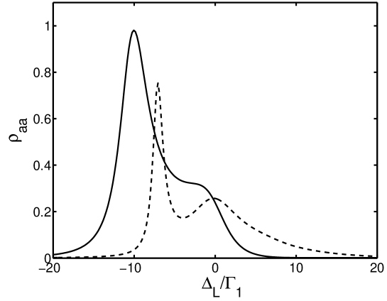
Figure 13: The steady-state population of the maximally entangled antisymmetric state $|{a}\rangle$ for $\Omega=10\Gamma_{1},\Omega_{12}=10\Gamma_{1}$ and $\Gamma_{2}=\Gamma_{1},\Delta=\Gamma_{1}$ (solid line), $\Gamma_{2}=2\Gamma_{1},\Delta=0$ (dashed line).

We illustrate this effect in Fig. 13, where we plot the steady-state population of the maximally entangled state $|{a}\rangle$ as a function of $\Delta_{L}$ for two different types of nonidentical atoms. In the first case the atoms have the same damping rates $(\Gamma_{1}=\Gamma_{2})$ but different transition frequencies $(\Delta\neq 0)$, while in the second case the atoms have the same frequencies $(\Delta=0)$ but different damping rates $(\Gamma_{1}\neq\Gamma_{2})$. It is seen from Fig. 13 that in both cases the antisymmetric state can be populated even if is not directly driven from the ground state. The population is transferred to $|{a}\rangle$ through the coherent interaction $\Delta_{c}$ which leaves the other excited states completely unpopulated.

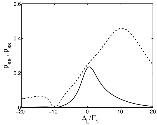
Figure 14: The steady-state populations of the upper state $|{e}\rangle$ (solid line) and the symmetric state $|{s}\rangle$ (dashed line) for $\Gamma_{2}=\Gamma_{1},\Omega=10\Gamma_{1},\Omega_{12}=10\Gamma_{1}$ and $\Delta=\Gamma_{1}$.

This is shown in Fig. 14, where we plot the steady-state populations $\rho_{ss}$ and $\rho_{ee}$ of the states $|{s}\rangle$ and $|{e}\rangle$. It is apparent from Fig. 14 that at $\Delta_{L}=-\Omega_{12}$ the states $|{s}\rangle$ and $|{e}\rangle$ are not populated. However, the population is not entirely trapped in the antisymmetric state $|{a}\rangle$, but rather in a linear superposition of the antisymmetric and ground states. This is illustrated in Fig. 15, where we plot the steady-state population $\rho_{aa}$ for the same parameters as in Fig. 14, but different $\Omega$. Clearly, for a small $\Omega$ the steady-state population $\rho_{aa}\approx\frac{1}{2}$, and the amount of the population increases with increasing $\Omega$. The population $\rho_{aa}$ attains the maximum value $\rho_{aa}\approx 1$ for a very strong driving field.

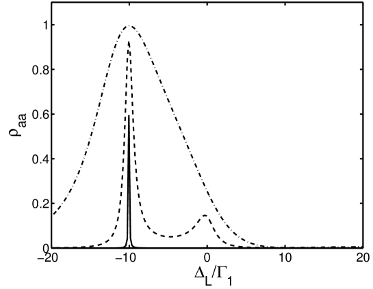
Figure 15: The steady-state population of the antisymmetric state $|{a}\rangle$ for $\Gamma_{2}=\Gamma_{1},\Omega_{12}=10\Gamma_{1},\Delta=\Gamma_{1}$ and different $\Omega$: $\Omega=\Gamma_{1}$ (solid line), $\Omega=5\Gamma_{1}$ (dashed line), $\Omega=20\Gamma_{1}$ (dashed-dotted line).

This result shows that we can relatively easily prepare two nonidentical atoms in the maximally entangled antisymmetric state. The closeness of the prepared state to the ideal one is measured by the fidelity $F$. Here $F$ is equal to the obtained maximum population in the state $\left|a\right\rangle$. For $\Omega\gg\Gamma$ the fidelity of the prepared state is maximal, equal to 1. As we have already mentioned, the system has the advantage that the maximally entangled state $\left|a\right\rangle$ does not decay, i.e. is a decoherence-free state.

7.2.3 Atom-cavity-field interaction

There have been several proposals to generate the antisymmetric state $|{a}\rangle$ in a system of two identical atoms interacting with a single-mode cavity field. In this case, collective effects arise from the interaction between the atoms induced by a strong coupling of the atoms to the cavity mode. An excited atom emits a photon into the cavity mode that is almost immediately absorbed by the second atom. Plenio et al. [155] have considered a system of two atoms trapped inside an optical cavity and separated by a distance much larger than the optical wavelength. This allows for the selective excitation of only one of the atoms. In this scheme the generation of the antisymmetric state relies on the concept of conditional dynamics due to continuous observation of the cavity field. If only one atom is excited and no photon is detected outside the cavity, the atoms are prepared in a dark state [156], which is equivalent to the antisymmetric state $|{a}\rangle$.

In earlier studies, Phoenix and Barnett [157], Kudrayvtsev and Knight [158] and Cirac and Zoller [159] have analyzed two-atom Jaynes-Cummings models for a violation of Bell’s inequality, and have shown that the atoms moving across a single-mode cavity can be prepared in the antisymmetric state via the interaction with the cavity field. In this scheme, the preparation of the antisymmetric state takes place in two steps. In the first step, one atom initially prepared in its excited state $|{e_{1}}\rangle$ is sent through a single-mode cavity being in the vacuum state $|{0}\rangle_{c}$. During the interaction with the cavity mode, the atomic population undergoes the vacuum Rabi oscillations, and the interaction time was varied by selecting different atomic velocities. If the velocity of the atom is such that the interaction time of the atom with the cavity mode is equal to quarter of the vacuum Rabi oscillations, the state of the combined system, the atom plus the cavity mode, is a superposition state

$$|{a_{1}c}\rangle=\frac{1}{\sqrt{2}}\left(|{e_{1}}\rangle|{0}\rangle_{c}-|{g_{1}}\rangle|{1}\rangle_{c}\right)\ .$$ (194)

Hence, the state of the total system, two atoms plus the cavity mode, after the first atom has crossed the cavity is

$$|{\Psi_{1}}\rangle=\frac{1}{\sqrt{2}}\left(|{e_{1}}\rangle|{0}\rangle_{c}-|{g_{1}}\rangle|{1}\rangle_{c}\right)|{g_{2}}\rangle\ .$$ (195)

If we now send the second atom, being in its ground state, with the selected velocity such that during the interaction with the cavity mode the atom undergoes half of the vacuum Rabi oscillation, the final state of the system becomes

$$|{\Psi_{12}c}\rangle = \frac{1}{\sqrt{2}}\left(|{e_{1}}\rangle|{0}\rangle_{c}|{g_{2}}\rangle-|{g_{1}}\rangle|{0}\rangle_{c}|{e_{2}}\rangle\right)$$ (196)

$$= \frac{1}{\sqrt{2}}\left(|{e_{1}}\rangle|{g_{2}}\rangle-|{g_{1}}\rangle|{e_{2}}\rangle\right)|{0}\rangle_{c}=|{a}\rangle|{0}\rangle_{c}\ .$$

Thus, the final state of the system is a product state of the atomic antisymmetric state $|{a}\rangle$ and the vacuum state of the cavity mode. In this scheme the cavity mode is left in the vacuum state which prevents the antisymmetric state from any noise of the cavity. The scheme to entangle two atoms in a cavity, proposed by Cirac and Zoller [159], has recently been realized experimentally by Hagly et al. [33].

Gerry [160] has proposed a similar method based on a dispersive interaction of the atoms with a cavity mode prepared in a coherent state $|{\alpha}\rangle$. The atoms enter the cavity in superposition states

$$|{a_{1}}\rangle = \frac{1}{\sqrt{2}}\left(|{e_{1}}\rangle+i|{g_{1}}\rangle\right)\ ,$$

$$|{a_{2}}\rangle = \frac{1}{\sqrt{2}}\left(|{e_{2}}\rangle-i|{g_{2}}\rangle\right)\ .$$ (197)

After passage of the second atom, the final state of the system is

$$|{\Psi_{12}c}\rangle = \frac{1}{2}\left\{\left(|{g_{1}}\rangle|{g_{2}}\rangle+|{e_{1}}\rangle|{e_{2}}\rangle\right)|{-\alpha}\rangle\right.$$ (198)

$$+\left.i\left(|{e_{1}}\rangle|{g_{2}}\rangle-|{g_{1}}\rangle|{e_{2}}\rangle\right)|{\alpha}\rangle\right\}\ .$$

Thus, if the cavity field is measured and found in the state $|{\alpha}\rangle$, the atoms are in the antisymmetric state. If the cavity field is found in the state $|{-\alpha}\rangle$, the atoms are in the entangled state

$$|{\Psi_{12}(-\alpha)}\rangle=\frac{1}{2}\left(|{g_{1}}\rangle|{g_{2}}\rangle+|{e_{1}}\rangle|{e_{2}}\rangle\right)\ .$$ (199)

The state (199) is called as a two photon entangled state. In section 9, we will discuss another method of preparing the system in the two-photon entangled state based on the interaction of two atoms with a squeezed vacuum field.

7.3 Entanglement of two distant atoms

In the previous subsection, we have discussed different excitation processes which can prepare two atoms in the antisymmetric state. The analysis involved single mode cavities, but ignored spontaneous emission from the atoms and the cavity damping. Here, we will extend this analysis to include spontaneous emission from the atoms and the cavity damping [161]. We will show that two atoms separated by an arbitrary distance $r_{12}$ and interacting with a strongly damped cavity mode can behave as the Dicke model even if there is no assumed interaction between the atoms.

Consider two identical atoms separated by a large distance such that $\Gamma_{12}\approx 0$ and $\Omega_{12}\approx 0$. The interatomic axis is oriented perpendicular to the direction of the cavity mode (cavity axis) which is driven by an external coherent laser field of the Rabi frequency $\Omega$. The atoms are coupled to the cavity mode with coupling constant $g$, and damped at the rate $\Gamma$ by spontaneous emission to modes other than the privileged cavity mode. For simplicity, we assume that the frequencies of the laser field $\omega_{L}$ and the cavity mode $\omega_{c}$ are both equal to the atomic transition frequency $\omega_{0}$. The master equation for the density operator $\hat{\rho}_{ac}$ of the system of two atoms plus cavity field has the form

$$\frac{\partial\hat{\rho}_{ac}}{\partial t} = -\frac{1}{2}i\Omega\left[\hat{a}+\hat{a}^{\dagger},\hat{\rho}_{ac}\right]-\frac{1}{2}ig\left[S^{-}\hat{a}^{\dagger}+\hat{a}S^{+},\hat{\rho}_{ac}\right]$$ (200)

$$-\frac{1}{2}\Gamma\hat{L}_{a}\hat{\rho}_{ac}-\frac{1}{2}\Gamma_{c}\hat{L}_{c}\hat{\rho}_{ac}\ ,$$

where

$$\hat{L}_{a}\hat{\rho}_{ac} = \sum_{i=1}^{2}\left(\hat{\rho}_{ac}S_{i}^{+}S_{i}^{-}+S_{i}^{+}S_{i}^{-}\hat{\rho}_{ac}-2S_{i}^{-}\hat{\rho}_{ac}S_{i}^{+}\right)\ ,$$

$$\hat{L}_{c}\hat{\rho}_{ac} = \hat{a}^{\dagger}\hat{a}\hat{\rho}_{ac}+\hat{\rho}_{ac}\hat{a}^{\dagger}\hat{a}-2\hat{a}\hat{\rho}_{ac}\hat{a}^{\dagger}\ ,$$ (201)

are operators representing the damping of the atoms by spontaneous emission and of the field by cavity decay, respectively; $\hat{a}$ and $\hat{a}^{\dagger}$ are the cavity-mode annihilation and creation operators, $S^{\pm}=S^{\pm}_{1}+S^{\pm}_{2}$ are collective atomic operators, and $\Gamma_{c}$ is the cavity damping rate.

To explore the dynamics of the atoms, we assume the ”bad-cavity” limit of $\Gamma_{c}\gg g\gg\Gamma$. This enables us to adiabatically eliminate the cavity mode and obtain a master equation for the reduced density operator of the atoms. We make the unitary transformation

$$\hat{\rho}_{T} = \hat{D}(-\eta)\hat{\rho}_{ac}\hat{D}(\eta)\ ,$$ (202)

where

$$\hat{D}(\eta)=e^{\eta\left(\hat{a}+\hat{a}^{\dagger}\right)}$$ (203)

is the displacement operator, and $\eta=\Omega/\Gamma_{c}$.

The master equation for the transformed operator reduces to

$$\frac{\partial\hat{\rho}_{T}}{\partial t} = \frac{1}{2}ig\eta\left[S^{+}+S^{-},\hat{\rho}_{T}\right]-\frac{1}{2}ig\left[S^{-}\hat{a}^{\dagger}+\hat{a}S^{+},\hat{\rho}_{T}\right]$$ (204)

$$-\frac{1}{2}\Gamma\hat{L}_{a}\hat{\rho}_{T}-\frac{1}{2}\Gamma_{c}\hat{L}_{c}\hat{\rho}_{T}\ .$$

We now introduce the photon number representation for the density operator $\hat{\rho}_{T}$ with respect to the cavity mode

$$\hat{\rho}_{T}=\sum_{m,n=0}^{\infty}\rho_{mn}|{m}\rangle\langle{n}|\ ,$$ (205)

where $\rho_{mn}$ are the density matrix elements in the basis of the photon number states of the cavity mode. Since the cavity mode is strongly damped, we can neglect populations of the highly excited cavity modes and limit the expansion to $m,n=1$. Under this approximation, the master equation (204) leads to the following set of coupled equations of motion for the density matrix elements

$$\dot{\rho}_{00} = \hat{L}\rho_{00}-\frac{1}{2}ig\left(S^{+}\rho_{10}-\rho_{01}S^{-}\right)+\Gamma_{c}\rho_{11}\ ,$$

$$\dot{\rho}_{10} = \hat{L}\rho_{10}-\frac{1}{2}ig\left(S^{-}\rho_{00}-\rho_{11}S^{-}\right)-\frac{1}{2}\Gamma_{c}\rho_{10}\ ,$$

$$\dot{\rho}_{11} = \hat{L}\rho_{11}-\frac{1}{2}ig\left(S^{-}\rho_{01}-\rho_{10}S^{+}\right)-\Gamma_{c}\rho_{11}\ ,$$ (206)

where $\hat{L}\rho_{ij}=\frac{1}{2}ig\eta\left[S^{+}+S^{-},\rho_{ij}\right]-\frac{1}{2}\Gamma\hat{L}_{a}\rho_{ij}$.

We note that the field-matrix elements $\rho_{mn}$ are still operators with respect to the atoms. Moreover

$$\rho_{00}+\rho_{11}={\rm Tr}_{F}\left(\hat{\rho}_{T}\right)=\hat{\rho}$$ (207)

is the reduced density operator of the atoms.

For the case of a strong cavity damping the most populated state of the cavity field is the ground state $|{0}\rangle$, and then we can assume that the coherence $\rho_{10}$ changes slowly in time, so that we can take $\dot{\rho}_{10}=0$. Hence, we find that

$$\rho_{10}\approx-\frac{ig}{\Gamma_{c}}\left(S^{-}\rho_{00}-\rho_{11}S^{-}\right)\ .$$ (208)

Substituting this solution to $\dot{\rho}_{00}$ and $\dot{\rho}_{11}$, we get

$$\dot{\rho}_{00} = \hat{L}\rho_{00}+\Gamma_{c}\rho_{11}-\frac{g^{2}}{2\Gamma_{c}}\left(S^{+}S^{-}\rho_{00}+\rho_{00}S^{+}S^{-}-2S^{+}\rho_{11}S^{-}\right)\ ,$$

$$\dot{\rho}_{11} = \hat{L}\rho_{11}-\Gamma_{c}\rho_{11}+\frac{g^{2}}{2\Gamma_{c}}\left(2S^{-}\rho_{00}S^{+}-S^{-}S^{+}\rho_{11}-\rho_{11}S^{-}S^{+}\right)\ .$$ (209)

Adding these two equations together and neglecting population of the state $|{1}\rangle$, we obtain the master equation for the reduced density operator of the atoms as

$$\frac{\partial\hat{\rho}}{\partial t} = \frac{1}{2}ig\eta\left[S^{+}+S^{-},\hat{\rho}\right]-\frac{1}{2}\Gamma\hat{L}_{a}\hat{\rho}$$ (210)

$$-\frac{g^{2}}{2\Gamma_{c}}\left(S^{+}S^{-}\hat{\rho}+\hat{\rho}S^{+}S^{-}-2S^{-}\hat{\rho}S^{+}\right)\ .$$

The first term in Eq. (210) describes the interaction of the atoms with the driving field of an effective Rabi frequency $g\eta$. The second term represents the usual damping of the atoms by spontaneous emission, whereas the last term describes the damping of the collective system with an effective damping rate $g^{2}/\Gamma_{c}$. If we choose the parameters such that the collective damping is much larger than the spontaneous rates of the single atoms, the second term in Eq. (210) can be ignored, and then the master equation (210) describes the time evolution of the collective two-atom system. Thus, two independent atoms located inside a strongly damped one-mode cavity behave as a single collective small sample model (Dicke model) with the damping rate $g^{2}/\Gamma_{c}$. This model, however, requires that the atoms are strongly coupled to the cavity mode $(g\gg\Gamma)$ and are located inside the cavity such that the interatomic axis is perpendicular to the direction of the cavity mode and the driving field.

7.4 Preparation of a superposition of the antisymmetric and the ground states

In the section 7.2.2, we have shown that two nonidentical two-level atoms can be prepared in an arbitrary superposition of the maximally entangled antisymmetric state $|{a}\rangle$ and the ground state $|{g}\rangle$

$$|{\Phi}\rangle=\gamma|{a}\rangle+\sqrt{1-|\gamma|^{2}}|{g}\rangle\ .$$ (211)

However, the preparation of the superposition state requires that the atoms have different transition frequencies. Recently, Beige et al. [162] have proposed a scheme in which the superposition state $|{\Phi}\rangle$ can be prepared in a system of two identical atoms placed at fixed positions inside an optical cavity.

Here, we discuss an alternative scheme where the superposition state $|{\Phi}\rangle$ can be generated in two identical atoms driven in free space by a coherent laser field. This can happen when the atoms are in nonequivalent positions in the driving field, i.e. the atoms experience different intensities and phases of the driving field. For a comparison, we first consider a specific geometry for the driving field, namely that the field is propagated perpendicularly to the atomic axis $(\vec{k}_{L}\cdot\vec{r}_{12}=0)$. We find from Eq. (159), that in this case the collective states are populated with the population distribution $\rho_{ee}=\rho_{aa}<\rho_{ss}$. The population distribution changes dramatically when the driving field propagates in directions different from perpendicular to the interatomic axis [85, 90, 91]. In this situation the populations strongly depend on the interatomic separation and the detuning $\Delta_{L}$. This can produce the interesting modification that the collective states can be selectively populated. We show this by solving numerically the system of 15 equations for the density matrix elements. The populations are plotted against the detuning $\Delta_{L}$ in Fig. 16 for the laser field propagating in the direction of the interatomic axis. We see from Fig. 16 that the collective states $|{s}\rangle$ and $|{e}\rangle$ are populated at $\Delta_{L}=0$ and $\Delta_{L}=\Omega_{12}$. The antisymmetric state is significantly populated at $\Delta_{L}=-\Omega_{12}$, and at this detuning the populations of the states $|{s}\rangle$ and $|{e}\rangle$ are close to zero. Since $\rho_{aa}<1$, the population is distributed between the antisymmetric and the ground states, and therefore at $\Delta_{L}=-\Omega_{12}$ the system is in a superposition of the maximally entangled state $|{a}\rangle$ and the ground state $|{g}\rangle$.

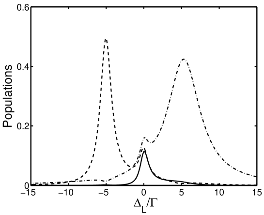
Figure 16: The steady-state populations of the collective atomic states of two identical atoms as a function of $\Delta_{L}$ for the driving field propagating in the direction of the interatomic axis, $\Omega=2.5\Gamma$, $r_{12}/\lambda=0.08$ and $\bar{\mu}\perp\bar{r}_{12}$: $\rho_{ee}$ (solid line), $\rho_{aa}$ (dashed line), $\rho_{ss}$ (dashed-dotted line).

Turchette et al. [32] have recently realized experimentally a superposition state of the ground state and a non-maximally entangled antisymmetric state in two trapped ions. In the experiment two trapped barium ions were sideband cooled to their motional ground states. Transitions between the states of the ions were induced by Raman pulses using co-propagating lasers. The ions were at positions that experience different Rabi frequencies $\Omega_{1}$ and $\Omega_{2}$ of the laser fields. By preparing the initial motional ground state with one ion excited $|{e_{1}}\rangle|{g_{2}}\rangle|{0}\rangle$, and applying the laser fields for a time $t$, the following entangled state $|{\Psi\left(t\right)}\rangle$ was created

$$|{\Psi\left(t\right)}\rangle = -\frac{i\Omega_{2}}{\Omega}\sin\left(\Omega t\right)|{g}\rangle|{1}\rangle+\left\{\left[\frac{\Omega_{2}^{2}}{\Omega^{2}}\left(\cos\Omega t-1\right)+1\right]|{e_{1}}\rangle|{g_{2}}\rangle\right.$$ (212)

$$+\left.\left[\frac{\Omega_{1}\Omega_{2}}{\Omega^{2}}\left(\cos\Omega t-1\right)\right]|{g_{1}}\rangle|{e_{2}}\rangle\right\}|{0}\rangle\ ,$$

where $\Omega^{2}=\Omega_{1}^{2}+\Omega_{2}^{2}$.

For $\Omega t=\pi$ the entangled state (212) reduces to a non-maximally entangled antisymmetric state

$$|{\Psi_{a}}\rangle=\left[\frac{\Omega_{1}^{2}-\Omega_{2}^{2}}{\Omega^{2}}|{e_{1}}\rangle|{g_{2}}\rangle-\frac{2\Omega_{1}\Omega_{2}}{\Omega^{2}}|{g_{1}}\rangle|{e_{2}}\rangle\right]|{0}\rangle\ .$$ (213)

Franke et al. [163] have proposed to use the non-maximally entangled state (213) to demonstrate the intrinsic difference between quantum and classical information transfers. The difference arises from the different ways in which the probabilities occur and is particularly clear in terms of entangled states.

8 Detection of the entangled states

In this section we describe two possible methods for detection of entangled states of two interacting atoms. One is the observation of angular intensity distribution of the fluorescence field emitted by the system of two interacting atoms. The other is based on quantum interference in which one observes interference pattern of the emitted field. Beige et al. [18] have proposed a scheme, based on the quantum Zeno effect, to observe a decoherence-free state in a system of two three-level atoms located inside an optical cavity. The two schemes discussed here involve two two-level atoms in free space.

8.1 Angular fluorescence distribution

It is well known that the fluorescence field emitted from a two-atom system exhibits strong directional properties [11, 47, 91, 149]. This property can be used to detect an internal state of two interacting atoms. To show this, we consider the fluorescence intensity, defined in Eq. (73), that in terms of the density matrix elements of the collective atomic system can be written as

$$I\left(\vec{R},t\right) = u(\vec{R})\left\{\left(\rho_{ee}+\rho_{ss}\right)\left[1+\cos\left(kr_{12}\cos\theta\right)\right]\right.$$ (214)

$$+\left.\left(\rho_{ee}+\rho_{aa}\right)\left[1-\cos\left(kr_{12}\cos\theta\right)\right]\right.$$

$$+\left.i\left(\rho_{sa}-\rho_{as}\right)\sin\left(kr_{12}\cos\theta\right)\right\}\ ,$$

where $\theta$ is the angle between the observation direction $\vec{R}$ and the vector $\vec{r}_{12}$.

The first term in Eq. (214) arises from the fluorescence emitted on the $|{e}\rangle\rightarrow|{s}\rangle\rightarrow|{g}\rangle$ transitions, which involve the symmetric state. The second term arises from the $|{e}\rangle\rightarrow|{a}\rangle\rightarrow|{g}\rangle$ transitions through the antisymmetric state. These two terms describe two different channels of transitions for which the angular distribution is proportional to $\left[1\pm\cos\left(kr_{12}\cos\theta\right)\right]$. The last term in Eq. (214) originates from interference between these two radiation channels. It is evident from Eq. (214) that the angular distribution of the fluorescence field depends on the population of the entangled states $|{s}\rangle$ and $|{a}\rangle$. Moreover, independent of the interatomic separation $r_{12}$, the antisymmetric state does not radiate in the direction perpendicular to the atomic axis, as for $\theta=\pi/2$ the factor $\left[1-\cos\left(kr_{12}\cos\theta\right)\right]$ vanishes. In contrast, the symmetric state radiates in all directions. Hence, the spatial distribution of the fluorescence field is not spherical unless $\rho_{ss}=\rho_{aa}$ and then the angular distribution is spherically symmetric independent of the interatomic separation. Therefore, an asymmetry in the angular distribution of the fluorescence field would be a compelling evidence that the entangled states $|{s}\rangle$ and $|{a}\rangle$ are not equally populated. If the fluorescence is detected in the direction perpendicular to the interatomic axis the observed intensity (if any) would correspond to the fluorescence field emitted from the symmetrical state $|{s}\rangle$ and/or the upper state $|{e}\rangle$. On the other hand, if there is no fluorescence detected in the direction perpendicular to the atomic axis, the population is entirely in a superposition of the antisymmetric state $|{a}\rangle$ and the ground state $|{g}\rangle$.

Guo and Yang [164, 165] have analyzed spontaneous decay from two atoms initially prepared in an entangled state. They have shown that the time evolution of the population inversion, which is proportional to the total radiation intensity (75), depends on the degree of entanglement of the initial state of the system. In Sections 4.1.1 and 4.1.2, we have shown that in the case of two non-identical atoms the time evolution of the total radiation intensity $I\left(t\right)$ can exhibit quantum beats which result from the presence of correlations between the symmetric and antisymmetric states. In fact, quantum beats are present only if initially the system is in a non-maximally entangled state, and no quantum beats are predicted for maximally entangled as well as unentangled states.

8.2 Interference pattern with a dark center

An alternative way to detect entangled states of a two-atom system is to observe an interference pattern of the fluorescence field emitted in the direction $\vec{R}$, not necessary perpendicular to the interatomic axis.

This scheme is particularly useful for detection of the symmetric or the antisymmetric state. To show this, we consider the visibility in terms of the density matrix elements of the collective atomic system as

$${\cal{V}}=\frac{\rho_{ss}-\rho_{aa}}{\rho_{ss}+\rho_{aa}+2\rho_{ee}}\ .$$ (215)

This simple formula shows that the sign of ${\cal{V}}$ depends on the population difference between the symmetric and antisymmetric states. For $\rho_{ss}>\rho_{aa}$ the visibility ${\cal{V}}$ is positive, and then the interference pattern exhibits a maximum (bright center), whereas for $\rho_{ss}<\rho_{aa}$ the visibility ${\cal{V}}$ is negative and then there is a minimum (dark center). The optimum positive (negative) value is ${\cal{V}}=1$ $({\cal{V}}=-1)$, and there is no interference pattern when ${\cal{V}}=0$. The later happens when $\rho_{ss}=\rho_{aa}$.

Similar to the fluorescence intensity distribution, the visibility can provide an information about the entangled states of a two-atom system. When the system is prepared in the antisymmetric state or in a superposition of the antisymmetric and the ground states, $\rho_{ss}=\rho_{ee}=0$, and then the visibility has the optimum negative value ${\cal{V}}=-1$. On the other hand, when the system is prepared in the symmetric state or in a linear superposition of the symmetric and ground states, the visibility has the maximum positive value ${\cal{V}}=1$.

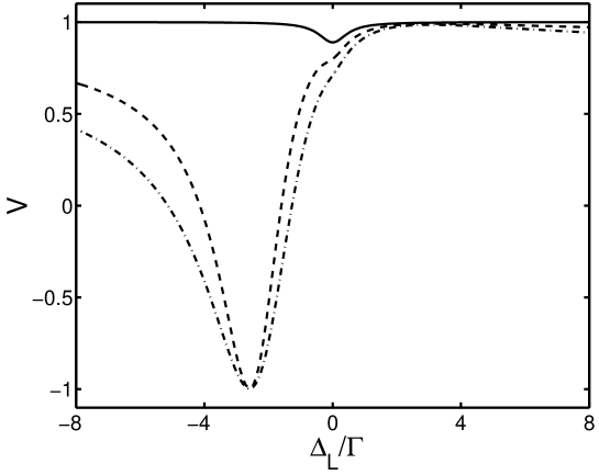
Figure 17: The visibility $V$ as a function of $\Delta_{L}$ for $r_{12}=0.1\lambda,\Omega=0.5\Gamma$ and various angles $\theta_{L}$; $\theta_{L}=\pi/2$ (solid line), $\theta_{L}=\pi/4$ (dashed line), $\theta_{L}=0$ (dashed-dotted line).

The earliest theoretical studies of the fringe visibility involved a coherent driving field which produces an interference pattern with a bright center. Recently, Meyer and Yeoman [166] have shown that in contrast to the coherent excitation, the incoherent field produces an interference pattern with a dark center. Dung and Ujihara [149] have shown that the fringe contrast factor can be negative for spontaneous emission from two undriven atoms, with initially one atom excited. Interference pattern with a dark center can also be obtained with a coherent driving field [147]. This happens when the atoms experience different phases and/or intensities of the driving field. To show this, we solve numerically the master equation (42) for the steady-state density matrix elements of the driven system of two atoms. The visibility $V$ is plotted in Fig. 17 as a function of the detuning $\Delta_{L}$ for $r_{12}=0.1\lambda,\Omega=0.25\Gamma$ and various angles $\theta_{L}$ between the interatomic axis and the direction of propagation of the laser field. The visibility $V$ is positive for most values of $\Delta_{L}$, except $\Delta_{L}\approx-\Omega_{12}$. At this detuning the parameter $V$ is negative and reaches the optimum negative value $V=-1$ indicating that the system produces interference pattern with a dark center. In Fig. 18, we plot the populations of the symmetric and antisymmetric states for the same parameters as in Fig 17. It is evident from Fig. 18 that at $\Delta_{L}=-\Omega_{12}$ the antisymmetric state is significantly populated, whereas the population of the symmetric state is close to zero. This population difference leads to negative values of $V$, as predicted by Eq. (215) and seen in Fig. 17. Experimental observation of the interference pattern with a dark center would be an interesting demonstration of the controled excitation of a two-atom system to the entangled antisymmetric state.

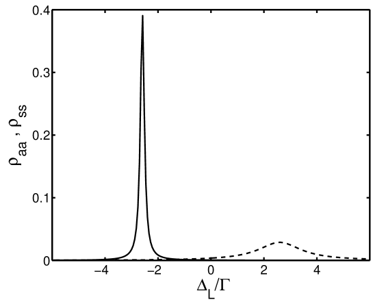
Figure 18: Populations of the symmetric and antisymmetric states for the same parameters as in Fig. 17, with $\theta_{L}=0$.

9 Two-photon entangled states

In our discussions to date on entanglement creation in two-atom systems, we have focused on different methods of creating entangled states of the form

$$|{\Psi}\rangle=c_{1}|{e_{1}}\rangle|{g_{2}}\rangle\pm c_{2}|{g_{1}}\rangle|{e_{2}}\rangle\ .$$ (216)

As we have shown in Sec. 3.1, entangled states of the above form are generated by the dipole-dipole interaction between the atoms and the preparation of these states is sensitive to the difference $\Delta$ between the atomic transition frequencies and to the atomic decay rates. These states are better known as the symmetric and antisymmetric collective atomic states.

Apart from the symmetric and antisymmetric states, there are two other collective states of the two-atom system: the ground state $|{g}\rangle=|{g_{1}}\rangle|{g_{2}}\rangle$ and the upper state $|{e}\rangle=|{e_{1}}\rangle|{e_{2}}\rangle$, which are also product states of the individual atomic states. These states are not affected by the dipole-dipole interaction $\Omega_{12}$.

In this section, we discuss a method of creating entanglement between these two states of the general form

$$|{\Upsilon}\rangle=c_{g}|{g}\rangle\pm c_{e}|{e}\rangle\ ,$$ (217)

where $c_{g}$ and $c_{e}$ are transformation parameters such that $|c_{g}|^{2}+|c_{e}|^{2}=1$. The entangled states of the form (217) are known in literature as pairwise atomic states [24, 25, 26, 27] or multi-atom squeezed states [23]. According to Eq. (67), the collective ground and excited states are separated in energy by $2\hbar\omega_{0}$, and therefore we can call the states $|{\Upsilon}\rangle$ as two-photon entangled (TPE) states.

The two-photon entangled states cannot be generated by a simple coherent excitation. A coherent field applied to the two-atom system couples to one-photon transitions. The problem is that coherent excitation populates not only the upper state $|{e}\rangle$ but also the intermediate states $|{s}\rangle$ and $|{a}\rangle$, see Eq. (159). The two-photon entangled states (217) are superpositions of the collective ground and excited states with no contribution from the intermediate collective states $|{s}\rangle$ and $|{a}\rangle$.

The two-photon behavior of the entangled states (217) suggests that the simplest technique for generating the TPE states would be by applying a two-photon excitation process. An obvious candidate is a squeezed vacuum field which is characterized by strong two-photon correlations which would enable the transition $|{g}\rangle\rightarrow|{e}\rangle$ to occur effectively in a single step without populating the intermediate states. We will illustrate this effect by analyzing the populations of the collective atomic states of a two-atom system interacting with a squeezed vacuum field.

9.1 Populations of the entangled states in a squeezed vacuum

The general master equation (36) allows us to calculate the populations of the collective atomic states and coherences, which gives information about the stationary state of a two-atom system. We first consider a system of two identical atoms, separated by an arbitrary distance $r_{12}$ and interacting with a squeezed vacuum field. For simplicity, we assume that the carrier frequency $\omega_{s}$ of the squeezed vacuum field is resonant to the atomic transition frequency $\omega_{0}$, and the squeezed field is perfectly matched to the atoms, $D(\omega_{s})=1$ and $\theta_{s}=\pi$.

From the master equation (36), we find the following equations of motion for the populations of the collective states and the two-photon coherences of the collective system of two identical atoms

$$\dot{\rho}_{ee} = -2\Gamma\left(\tilde{N}+1\right)\rho_{ee}+\tilde{N}\left[\left(\Gamma+\Gamma_{12}\right)\rho_{ss}+\left(\Gamma-\Gamma_{12}\right)\rho_{aa}\right]+\Gamma_{12}|\tilde{M}|\rho_{u}\ ,$$

$$\dot{\rho}_{ss} = \left(\Gamma+\Gamma_{12}\right)\left\{\tilde{N}-\left(3\tilde{N}+1\right)\rho_{ss}-\tilde{N}\rho_{aa}+\rho_{ee}-|\tilde{M}|\rho_{u}\right\}\ ,$$

$$\dot{\rho}_{aa} = \left(\Gamma-\Gamma_{12}\right)\left\{\tilde{N}-\left(3\tilde{N}+1\right)\rho_{aa}-\tilde{N}\rho_{ss}+\rho_{ee}+|\tilde{M}|\rho_{u}\right\}\ ,$$

$$\dot{\rho}_{u} = 2\Gamma_{12}|\tilde{M}|-\left(2\tilde{N}+1\right)\Gamma\rho_{u}$$ (218)

$$-2|\tilde{M}|\left[\left(\Gamma+2\Gamma_{12}\right)\rho_{ss}-\left(\Gamma-2\Gamma_{12}\right)\rho_{aa}\right]\ ,$$

where $\tilde{N}=\tilde{N}\left(\omega_{0}\right)$, $\tilde{M}=\tilde{M}\left(\omega_{0}\right)$ and $\rho_{u}=\rho_{eg}\exp(-i\phi_{s})+\rho_{ge}\exp(i\phi_{s})$.

It is seen from Eq. (218) that the evolution of the populations depends on the two-photon coherencies $\rho_{eg}$ and $\rho_{ge}$, which can transfer the population from the ground state $|{g}\rangle$ directly to the upper state $|{e}\rangle$ leaving the states $|{s}\rangle$ and $|{a}\rangle$ unpopulated. The evolution of the populations depends on $\Gamma_{12}$, but is completely independent of the dipole-dipole interaction $\Omega_{12}$.

Similar to the interaction with the ordinary vacuum, discussed in Sec. 3.1, the steady-state solution of Eqs. (218) depends on whether $\Gamma_{12}=\Gamma$ or $\Gamma_{12}\neq\Gamma$. Assuming that $\Gamma_{12}=\Gamma$ and setting the left-hand side of equations (218) equal to zero, we obtain the steady-state solutions for the populations and the two-photon coherence in the Dicke model. A straightforward algebraic manipulation of Eqs. (218) leads to the following steady-state solutions

$$\rho_{ee} = \frac{\tilde{N}^{2}\left(2\tilde{N}+1\right)-\left(2\tilde{N}-1\right)|\tilde{M}|^{2}}{\left(2\tilde{N}+1\right)\left(3\tilde{N}^{2}+3\tilde{N}+1-3|\tilde{M}|^{2}\right)}\ ,$$

$$\rho_{ss} = \frac{\tilde{N}\left(\tilde{N}+1\right)-|\tilde{M}|^{2}}{3\tilde{N}^{2}+3\tilde{N}+1-3|\tilde{M}|^{2}}\ ,$$

$$\rho_{u} = \frac{2|\tilde{M}|}{\left(2\tilde{N}+1\right)\left(3\tilde{N}^{2}+3\tilde{N}+1-3|\tilde{M}|^{2}\right)}\ .$$ (219)

The steady-state populations depend strongly on the squeezing correlations $\tilde{M}$. For a classical squeezed field with the maximal correlations $\tilde{M}=\tilde{N}$ the steady-state populations reduces to

$$\rho_{ss} = \frac{\tilde{N}}{3\tilde{N}+1}\ ,$$

$$\rho_{ee} = \frac{2\tilde{N}^{2}}{\left(2\tilde{N}+1\right)\left(3\tilde{N}+1\right)}\ .$$ (220)

It is easily to check that in this case the populations obey a Boltzmann distribution with $\rho_{gg}>\rho_{ss}>\rho_{ee}$. Moreover, in the limit of low intensities $(\tilde{N}\ll 1)$ of the field, the population $\rho_{ee}$ is proportional to $\tilde{N}^{2}$, showing that in classical fields the population exhibits a quadratic dependence on the intensity.

The population distribution is qualitatively different for a quantum squeezed field with the maximal correlations $|\tilde{M}|^{2}=\tilde{N}(\tilde{N}+1)$. In this case, the stationary populations of the excited collective states are

$$\rho_{ss} = 0\ ,$$

$$\rho_{ee} = \frac{\tilde{N}}{\left(2\tilde{N}+1\right)}\ .$$ (221)

Clearly, the symmetric state is not populated. In this case the populations no longer obey the Boltzmann distribution. The population is distributed only between the ground state $|{g}\rangle$ and the upper state $|{e}\rangle$. Moreover, it can be seen from Eq. (221) that for a weak quantum squeezed field the population $\rho_{ee}$ depends linearly on the intensity. This distinctive feature reflects the direct modifications of the two-photon absorption that the nonclassical photon correlations enable the transition $|{g}\rangle\rightarrow|{e}\rangle$ to occurs in a ”single step” proportional to $\tilde{N}$. In other words, the nonclassical two-photon correlations entangle the ground state $|{g}\rangle$ and the upper state $|{e}\rangle$ with no contribution from the symmetric state $|{s}\rangle$.

The question we are interested in concerns the final state of the system and its purity. To answer this question, we apply Eq. (219) and find that in the steady-state, the density matrix of the system is given by

$$\hat{\rho} = \left(\begin{array}[]{ccc}\rho_{gg}&0&\rho_{ge}\\ 0&\rho_{ss}&0\\ \rho_{eg}&0&\rho_{ee}\end{array}\right)\ ,$$ (225)

where $\rho_{ij}$ are the non-zero steady-state density matrix elements.

It is evident from Eq. (225) that in the squeezed vacuum the density matrix of the system is not diagonal due to the presence of the two-photon coherencies $\rho_{ge}$ and $\rho_{eg}$. This indicates that the collective states $|{g}\rangle$, $|{s}\rangle$ and $|{e}\rangle$ are no longer eigenstates of the system. The density matrix can be rediagonalized by including $\rho_{eg}$ and $\rho_{ge}$ to give the new (entangled) states

$$|{\Upsilon_{1}}\rangle = \left[\left(P_{1}-\rho_{ee}\right)|{g}\rangle+\rho_{eg}|{e}\rangle\right]/\left[\left(P_{1}-\rho_{ee}\right)^{2}+\left|\rho_{eg}\right|^{2}\right]^{\frac{1}{2}}\ ,$$

$$|{\Upsilon_{2}}\rangle = \left[\rho_{ge}|{g}\rangle+\left(P_{2}-\rho_{gg}\right)|{e}\rangle\right]/\left[\left(P_{2}-\rho_{gg}\right)^{2}+\left|\rho_{eg}\right|^{2}\right]^{\frac{1}{2}}\ ,$$

$$|{\Upsilon_{3}}\rangle = |{s}\rangle\ ,$$ (226)

where the diagonal probabilities are

$$P_{1} = \frac{1}{2}\left(\rho_{gg}+\rho_{ee}\right)+\frac{1}{2}\left[\left(\rho_{gg}-\rho_{ee}\right)^{2}+4\left|\rho_{eg}\right|^{2}\right]^{\frac{1}{2}}\ ,$$

$$P_{2} = \frac{1}{2}\left(\rho_{gg}+\rho_{ee}\right)-\frac{1}{2}\left[\left(\rho_{gg}-\rho_{ee}\right)^{2}+4\left|\rho_{eg}\right|^{2}\right]^{\frac{1}{2}}\ ,$$

$$P_{3} = \rho_{ss}\ .$$ (227)

In view of Eqs. (221) and (226), it is easy to see that the squeezed vacuum causes the system to decay into entangled states which are linear superpositions of the collective ground state $|{g}\rangle$ and the upper state $|{e}\rangle$. The intermediate symmetric state remains unchanged under the squeezed vacuum excitation. In general, the states (226) are mixed states. However, for perfect correlations $|\tilde{M}|^{2}=\tilde{N}(\tilde{N}+1)$ the populations $P_{2}$ and $P_{3}$ are zero leaving the population only in the state $|{\Upsilon_{1}}\rangle$. Hence, the state $|{\Upsilon_{1}}\rangle$ is a pure state of the system of two atoms driven by a squeezed vacuum field. From Eqs. (226), we find that the pure entangled state $|{\Upsilon_{1}}\rangle$ is given by [167]

$$|{\Upsilon_{1}}\rangle=\frac{1}{\sqrt{2\tilde{N}+1}}\left[\sqrt{\tilde{N}+1}|{g}\rangle+\sqrt{\tilde{N}}|{e}\rangle\right]\ .$$ (228)

The pure state (228) is non-maximally entangled state, it reduces to a maximally entangled state for $\tilde{N}\gg 1$. The entangled state is analogous to the pairwise atomic state [24, 25, 26, 27] or the multi-atom squeezed state [23], (see also Ref. [29]), predicted in the small sample model of two coupled atoms.

The pure entangled state $|{\Upsilon_{1}}\rangle$ is characteristic not only of the two-atom Dicke model, but in general of the Dicke model of an even number of atoms [168]. The $N$-atom Dicke system interacting with a squeezed vacuum can decay to a state which the density operator is given by

$$\hat{\rho} = C_{n}\left(\mu S^{-}+\nu S^{+}\right)^{-1}\left(\mu S^{+}+\nu S^{-}\right)^{-1}\ ,$$ (229)

if $N$ is odd, or

$$\hat{\rho}=|{\Upsilon}\rangle\langle{\Upsilon}|\ ,$$ (230)

if $N$ is even, where $C_{n}$ is the normalization constant, $S^{\pm}$ are the collective atomic operators, $\mu^{2}=\nu^{2}+1=\tilde{N}+1$, and $|{\Upsilon}\rangle$ is defined by

$$\left(\mu S^{-}+\nu S^{+}\right)|{\Upsilon}\rangle=0\ .$$ (231)

Thus, for an even number of atoms the stationary state of the system is the pure pairwise atomic state.

9.2 Effect of the antisymmetric state on the purity of the system

The pure entangled state $|{\Upsilon_{1}}\rangle$ can be obtained for perfect matching of the squeezed modes to the atoms and interatomic separations much smaller than the optical wavelength. To achieve perfect matching, it is necessary to squeeze of all the modes to which the atoms are coupled. That is, the squeezed modes must occupy the whole $4\pi$ solid angle of the space surrounding the atoms. This is not possible to achieve with the present experiments in free space, and in order to avoid the difficulty cavity environments have been suggested [54, 55]. Inside a cavity the atoms interact strongly only with the privileged cavity modes. By the squeezing of these cavity modes, which occupy only a small solid angle about the cavity axis, it would be possible to achieve perfect matching of the squeezed field to the atoms.

There is, however, the practical problem to fulfil the second requirement that interatomic separations should be much smaller than the resonant wavelength. This assumption may prove difficult in experimental realization as with the present techniques two atoms can be trapped within distances of the order of a resonant wavelength [13, 14, 15, 16]. As we have shown in Sec. 3.1, the dynamics of such a system involve the antisymmetric state and are significantly different from the dynamics of the Dicke model.

For two atoms separated by an arbitrary distance $r_{12}$, the collective damping $\Gamma_{12}\neq\Gamma$, and then the steady-state solutions of Eqs. (218) are

$$\rho_{ee} = \frac{\tilde{N}^{2}}{\left(2\tilde{N}+1\right)^{2}}+\frac{a^{2}|\tilde{M}|^{2}\left(4\tilde{N}+1\right)}{G}\ ,$$

$$\rho_{ss} = \frac{\tilde{N}\left(\tilde{N}+1\right)}{\left(2\tilde{N}+1\right)^{2}}-\frac{a|\tilde{M}|^{2}\left[2\left(2\tilde{N}+1\right)^{2}-a\right]}{G}\ ,$$

$$\rho_{aa} = \frac{\tilde{N}\left(\tilde{N}+1\right)}{\left(2\tilde{N}+1\right)^{2}}+\frac{a|\tilde{M}|^{2}\left[2\left(2\tilde{N}+1\right)^{2}+a\right]}{G},$$

$$\rho_{u} = \frac{2a\left(2\tilde{N}+1\right)^{3}|\tilde{M}|}{G}\ ,$$ (232)

where $a=\Gamma_{12}/\Gamma$, and

$$G=\left(2\tilde{N}+1\right)^{2}\left\{\left(2\tilde{N}+1\right)^{4}+4|\tilde{M}|^{2}\left[a^{2}-\left(2\tilde{N}+1\right)^{2}\right]\right\}\ .$$ (233)

Figure 19: The steady-state populations of the collective atomic states as a function of $r_{12}$ for (a) quantum squeezed field with $|\tilde{M}|^{2}=\tilde{N}(\tilde{N}+1)$, (b) classical squeezed field with $|\tilde{M}|=\tilde{N}$, and $\tilde{N}=0.05$, $\bar{\mu}\perp\bar{r}_{12}$: $\rho_{ee}$ (solid line), $\rho_{aa}$ (dashed line), $\rho_{ss}$ (dashed-dotted line).

This result shows that the antisymmetric state is populated in the steady-state even for small interatomic separations $(\Gamma_{12}\approx\Gamma)$. For large interatomic separations $\Gamma_{12}\approx 0$, and then the symmetric and antisymmetric states are equally populated. When the interatomic separation decreases, the population of the state $|{a}\rangle$ increases, whereas the population of the state $|{s}\rangle$ decreases and $\rho_{ss}=0$ for very small interatomic separations. These features are illustrated in Fig. 19(a), where we plot the steady-state populations as a function of the interatomic separation for the maximally correlated quantum squeezed field. We see that the collective states are unequally populated and in the case of small $r_{12}$, the state $|{a}\rangle$ is the most populated state of the system, whereas the state $|{s}\rangle$ is not populated. In Fig. 19(b), we show the populations for the equivalent maximally correlated classical squeezed field, and in this case all states are populated independent of $r_{12}$.

This fact can lead to a destruction of the purity of the stationary state of the system. To show this, we calculate the quantity

$${\rm Tr}\left(\hat{\rho}^{2}\right)=\rho_{gg}^{2}+\rho_{ss}^{2}+\rho_{aa}^{2}+\rho_{ee}^{2}+\left|\rho_{u}\right|^{2}\ ,$$ (234)

which determines the purity of the system. Tr$(\hat{\rho}^{2})=1$ corresponds to a pure state of the system, while Tr$(\hat{\rho}^{2})<1$ corresponds to a mixed state. Tr$(\hat{\rho}^{2})=1/4$ describes a completely mixed state of the system. In Fig. 20, we display Tr$(\hat{\rho}^{2})$ as a function of the interatomic separation $r_{12}$ for perfect correlations $|\tilde{M}|^{2}=\tilde{N}(\tilde{N}+1)$ and various $\tilde{N}$. Clearly, the system is in a mixed state independent of the interatomic separation. Moreover, the purity decreases as $\tilde{N}$ increases.

Figure 20: Tr$(\hat{\rho}^{2})$ as a function of the interatomic separation for $|\tilde{M}|^{2}=\tilde{N}(\tilde{N}+1)$, $\bar{\mu}\perp\bar{r}_{12}$ and different $\tilde{N}$: $\tilde{N}=0.05$ (solid line), $\tilde{N}=0.5$ (dashed line), $\tilde{N}=5$ (dashed-dotted line).

For small interatomic separation, the mixed state of the system is composed of two states: the TPE state $|{\Upsilon_{1}}\rangle$ and the antisymmetric state $|{a}\rangle$. We illustrate this by diagonalizing the steady-state density matrix of the system

$$\hat{\rho} = \left(\begin{array}[]{cccc}\rho_{gg}&0&0&\rho_{ge}\\ 0&\rho_{aa}&0&0\\ 0&0&\rho_{ss}&0\\ \rho_{eg}&0&0&\rho_{ee}\end{array}\right)\ ,$$ (239)

from which we find the new (entangled) states

$$|{\Upsilon_{1}}\rangle = \left[\left(P_{1}-\rho_{ee}\right)|{g}\rangle+\rho_{eg}|{e}\rangle\right]/\left[\left(P_{1}-\rho_{ee}\right)^{2}+\left|\rho_{eg}\right|^{2}\right]^{\frac{1}{2}}\ ,$$

$$|{\Upsilon_{2}}\rangle = \left[\rho_{ge}|{g}\rangle+\left(P_{2}-\rho_{gg}\right)|{e}\rangle\right]/\left[\left(P_{2}-\rho_{gg}\right)^{2}+\left|\rho_{eg}\right|^{2}\right]^{\frac{1}{2}}\ ,$$

$$|{\Upsilon_{3}}\rangle = |{s}\rangle\ ,$$

$$|{\Upsilon_{4}}\rangle = |{a}\rangle\ ,$$ (240)

where the diagonal probabilities (populations of the entangled states) are

$$P_{1} = \frac{1}{2}\left(\rho_{gg}+\rho_{ee}\right)+\frac{1}{2}\left[\left(\rho_{gg}-\rho_{ee}\right)^{2}+4\left|\rho_{eg}\right|^{2}\right]^{\frac{1}{2}}\ ,$$

$$P_{2} = \frac{1}{2}\left(\rho_{gg}+\rho_{ee}\right)-\frac{1}{2}\left[\left(\rho_{gg}-\rho_{ee}\right)^{2}+4\left|\rho_{eg}\right|^{2}\right]^{\frac{1}{2}}\ ,$$

$$P_{3} = \rho_{ss}\ ,$$

$$P_{4} = \rho_{aa}\ .$$ (241)

Figure 21: Populations of the entangled states (240) as a function of the interatomic separation for (a) quantum squeezed field with $|\tilde{M}|^{2}=\tilde{N}(\tilde{N}+1)$, (b) classical squeezed field with $|\tilde{M}|=\tilde{N}$, and $\bar{\mu}\perp\bar{r}_{12}$, $\tilde{N}=0.5$. In both frames $P_{1}$ (solid line), $P_{2}$ (dashed line), $P_{3}$ (dashed-dotted line), $P_{4}$ (dotted line).

Note, that the states $|{\Upsilon_{1}}\rangle,|{\Upsilon_{2}}\rangle$ and $|{\Upsilon_{3}}\rangle$ are the same as for the small sample model, discussed in the preceding section. This means that the presence of the antisymmetric state does not affect the two-photon entangled states, but it can affect the population distribution between the states and the purity of the system. In Fig. 21, we plot the populations $P_{i}$ of the states $|{\Upsilon_{i}}\rangle$ as a function of the interatomic separation. The figure demonstrates that in the case of a quantum squeezed field the atoms are driven into a mixed state composed of only two entangled states $|{\Upsilon_{1}}\rangle$ and $|{a}\rangle$, and there is a vanishing probability that the system is in the states $|{\Upsilon_{2}}\rangle$ and $|{s}\rangle$. In contrast, for a classical squeezed field, shown in Fig. 21(b), the atoms are driven to a mixed state composed of all the entangled states.

Following the discussion presented in Sec. 3.1, we can argue that the system can decay to the pure TPE state $|{\Upsilon_{1}}\rangle$ with the interatomic separation included. This can happen when the observation time is shorter than $\Gamma^{-1}$. The antisymmetric state $\left|a\right\rangle$ decays on a time scale $\sim\left(\Gamma-\Gamma_{12}\right)^{-1}$, and for $\Gamma_{12}\approx\Gamma$ the decay rate of the antisymmetric state is much longer than $\Gamma^{-1}$. By contrast, the state $\left|s\right\rangle$ decays on a time scale $\sim\left(\Gamma+\Gamma_{12}\right)^{-1},$ which for $\Gamma_{12}\approx\Gamma$ is shorter than $\Gamma^{-1}$. Clearly, for observation times shorter than $\Gamma^{-1},$ the antisymmetric state does not participate in the interaction and the system reaches the steady-state only between the triplet states. Thus, for perfect matching of the squeezed modes to the atoms the symmetric state is not populated and then the system is in the pure TPE state $|{\Upsilon_{1}}\rangle$.

9.3 Two-photon entangled states for two non-identical atoms

We now extend the analysis of the population distribution in a squeezed vacuum to the case of two nonidentical atoms. For two nonidentical atoms with $\Delta\neq 0$ and $\Gamma_{1}=\Gamma_{2}=\Gamma$, the master equation (36) leads to the following equations of motion for the density matrix elements

$$\dot{\rho}_{ee} = -2\Gamma\left(\tilde{N}+1\right)\rho_{ee}+\tilde{N}\left[\Gamma\left(\rho_{ss}+\rho_{aa}\right)+\Gamma_{12}\left(\rho_{ss}-\rho_{aa}\right)e^{i\Delta t}\right]$$

$$+\Gamma_{12}|\tilde{M}|\left(\rho_{eg}e^{-i\left[2\left(\omega_{s}-\omega_{0}\right)t+\phi_{s}\right]}+\rho_{ge}e^{i\left[2\left(\omega_{s}-\omega_{0}\right)t+\phi_{s}\right]}\right)\ ,$$

$$\dot{\rho}_{ss} = \left(\Gamma+\Gamma_{12}e^{i\Delta t}\right)\left[\tilde{N}-\left(3\tilde{N}+1\right)\rho_{ss}-\tilde{N}\rho_{aa}+\rho_{ee}\right]$$

$$-\Gamma|\tilde{M}|\left(\rho_{eg}e^{-i\left[2\left(\omega_{s}-\omega_{1}\right)t+\phi_{s}\right]}+\rho_{ge}e^{i\left[2\left(\omega_{s}-\omega_{1}\right)t+\phi_{s}\right]}\right)$$

$$-\Gamma_{12}|\tilde{M}|\left(\rho_{eg}e^{-i\left[2\left(\omega_{s}-\omega_{0}\right)t+\phi_{s}\right]}+\rho_{ge}e^{i\left[2\left(\omega_{s}-\omega_{0}\right)t+\phi_{s}\right]}\right)\ ,$$

$$\dot{\rho}_{aa} = \left(\Gamma-\Gamma_{12}e^{i\Delta t}\right)\left[\tilde{N}-\left(3\tilde{N}+1\right)\rho_{aa}-\tilde{N}\rho_{ss}+\rho_{ee}\right]$$

$$+\Gamma|\tilde{M}|\left(\rho_{eg}e^{-i\left[2\left(\omega_{s}-\omega_{1}\right)t+\phi_{s}\right]}+\rho_{ge}e^{i\left[2\left(\omega_{s}-\omega_{1}\right)t+\phi_{s}\right]}\right)$$

$$-\Gamma_{12}|\tilde{M}|\left(\rho_{eg}e^{-i\left[2\left(\omega_{s}-\omega_{0}\right)t+\phi_{s}\right]}+\rho_{ge}e^{i\left[2\left(\omega_{s}-\omega_{0}\right)t+\phi_{s}\right]}\right)\ ,$$

$$\dot{\rho}_{eg} = \left(\dot{\rho}_{ge}\right)^{\ast}=\Gamma_{12}|\tilde{M}|e^{i\left[2\left(\omega_{s}-\omega_{1}\right)t+\phi_{s}\right]}-\left(2\tilde{N}+1\right)\Gamma\rho_{eg}$$ (242)

$$-\Gamma|\tilde{M}|e^{i\left[2\left(\omega_{s}-\omega_{1}\right)t+\phi_{s}\right]}\left(\rho_{ss}-\rho_{aa}\right)$$

$$-2\Gamma_{12}|\tilde{M}|e^{i\left[2\left(\omega_{s}-\omega_{0}\right)t+\phi_{s}\right]}\left(\rho_{ss}+\rho_{aa}\right)\ ,$$

where $\omega_{0}=\frac{1}{2}\left(\omega_{1}+\omega_{2}\right)$.

Equations (242) contain time-dependent terms which oscillate at frequencies exp$(\pm i\Delta t)$ and exp$[\pm 2i(\omega_{s}-\omega_{0})t+\phi_{s}]$. If we tune the squeezed vacuum field to the middle of the frequency difference between the atomic frequencies, i.e. $\omega_{s}=(\omega_{1}+\omega_{2})/2$, the terms proportional to exp$[\pm 2i(\omega_{s}-\omega_{0})t+\phi_{s}]$ become stationary in time. None of the other time dependent components is resonant with the frequency of the squeezed vacuum field. Consequently, for $\Delta\gg\Gamma$, the time-dependent components oscillate rapidly in time and average to zero over long times. Therefore, we can make a secular approximation in which we ignore the rapidly oscillating terms, and find the following steady-state solutions [169]

$$\rho_{ee} = \frac{1}{4}\left\{\frac{\left(2\tilde{N}-1\right)}{2\tilde{N}+1}+\frac{1}{\left[\left(2\tilde{N}+1\right)^{2}-4a^{2}|\tilde{M}|^{2}\right]}\right\}\ ,$$

$$\rho_{ss} = \rho_{aa}=\frac{1}{4}\left\{1-\frac{1}{\left[\left(2\tilde{N}+1\right)^{2}-4a^{2}|\tilde{M}|^{2}\right]}\right\}\ ,$$

$$\rho_{u} = \frac{2a|\tilde{M}|}{\left(2\tilde{N}+1\right)\left[\left(2\tilde{N}+1\right)^{2}-4a^{2}|\tilde{M}|^{2}\right]}\ .$$ (243)

Equations (243) are quite different from Eqs. (232) and show that in the case of non-identical atoms the symmetric and antisymmetric states are equally populated independent of the interatomic separation. These are, however, some similarities to the steady-state solutions of the Dicke model that for small interatomic separations $\rho_{ss}=\rho_{aa}\approx 0$, and then only the collective ground and the upper states are populated.

To conclude this section, we point out that by employing two spatially separated non-identical atoms of significantly different transition frequencies $(\Delta\gg\Gamma)$, it is possible to achieve the pure TPE state with the antisymmetric state fully participating in the interaction.

10 Mapping of entangled states of light on atoms

The generation of the pure TPE state is an example of mapping of a state of quantum correlated light onto an atomic system. The two-photon correlations contained in the squeezed vacuum field can be completely transferred to the atomic system and can be measured, for example, by detecting fluctuations of the fluorescence field emitted by the atomic system. Squeezing in the fluorescence field is proportional to the squeezing in the atomic dipole operators (spin squeezing) which, on the other hand, can be found from the steady-state solutions for the density matrix elements.

10.1 Mapping of photon correlations

Equation (243) shows that the collective damping parameter $\Gamma_{12}$ plays the role of a degree of the correlation transfer from the squeezed vacuum to the atomic system. For large interatomic separations, $\Gamma_{12}\approx 0$, and there is no transfer of the correlations to the system. In contrast, for very small separations, $\Gamma_{12}\approx\Gamma$, and then the correlations are completely transferred to the atomic system.

However, the complete transfer of the correlations does not necessary mean that the two-photon correlations are stored in the pure TPE state. This happens only for two nonidentical atoms in the Dicke model, where the steady-state is the pure TPE state. For identical atoms separated by a finite distance $r_{12}$ only a part of the correlations can be stored in the antisymmetric state. This can be shown, for example, by calculating of the interference pattern of the fluorescence field emitted by the system. Using the steady-state solutions (232), we find that the visibility in the interference pattern is given by [170]

$${\cal{V}}=-\frac{2a|\tilde{M}|^{2}}{\tilde{N}\left(2\tilde{N}+1\right)^{3}+2|\tilde{M}|^{2}\left[a^{2}+\left(2\tilde{N}+1\right)-\left(2\tilde{N}+1\right)^{2}\right]}\ .$$ (244)

Figure 22: The visibility ${\cal{V}}$ as a function of the interatomic separation $r_{12}$ for (a) a quantum squeezed field with $|\tilde{M}|^{2}=\tilde{N}(\tilde{N}+1)$, (b) a classical squeezed field with $|\tilde{M}|=\tilde{N}$, $\bar{\mu}\perp\bar{r}_{12}$ and different $\tilde{N}$: $\tilde{N}=0.05$ (solid line), $\tilde{N}=0.5$ (dashed line), $\tilde{N}=5$ (dashed-dotted line).

The visibility is negative indicating that the squeezing correlations are mostly stored in the antisymmetric state. In Fig. 22, we plot the visibility ${\cal{V}}$ as a function of the interatomic separation for a quantum squeezed field with $|\tilde{M}|^{2}=\tilde{N}(\tilde{N}+1)$, Fig. 22(a), and a classical squeezed field with $|\tilde{M}|=\tilde{N}$, Fig. 22(b). An interference pattern with a dark center is observed for small interatomic separations $(r_{12}<\lambda/2)$ and with the quantum squeezed field the visibility attains the maximal negative value of ${\cal{V}}\approx-0.7$ for $r_{12}<0.3\lambda$. According to Eq. (234), at these interatomic separations the antisymmetric state is the most populated state of the system. The value ${\cal{V}}=-0.7$ compared to the possible negative value ${\cal{V}}=-1$ indicates that $70\%$ of the squeezing correlations are stored in the antisymmetric state. In Fig. 22(b), we show the visibility for a classical squeezed field with $|\tilde{M}|=\tilde{N}$. The visibility is much smaller than that in the quantum squeezed field and vanishes when $\tilde{N}\rightarrow\infty$. In contrast, for the quantum squeezed field $V$ approaches $-1/2$ when $\tilde{N}\rightarrow\infty$. Thus, the visibility can provide the information about the degree of nonclassical correlations stored in the entangled state $|{a}\rangle$.

10.2 Mapping of the field fluctuations

The fluctuations of the electric field are determined by the normally ordered variance of the field operators as [29, 30, 31]

$$\langle:\left(\Delta E_{\theta}\right)^{2}:\rangle=\sum_{\vec{k}s}E_{k}\left(2\langle\hat{a}_{\vec{k}s}^{\dagger}\hat{a}_{\vec{k}s}\rangle+\langle\hat{a}_{\vec{k}s}\hat{a}_{\vec{k}s}\rangle e^{2i\theta}+\langle\hat{a}_{\vec{k}s}^{\dagger}\hat{a}_{\vec{k}s}^{\dagger}\rangle e^{-2i\theta}\right)\ .$$ (245)

Using the correlation functions (17) of the three-dimensional squeezed vacuum field and choosing $\theta=\pi/2$, the variance of the incident squeezed vacuum field can be written as

$$\left\langle:\left(\Delta E^{in}_{\pi/2}\right)^{2}:\right\rangle=2E_{0}\left(\tilde{N}-|\tilde{M}|\right)\ ,$$ (246)

where $E_{0}$ is a constant. Since $|\tilde{M}|=\sqrt{\tilde{N}(\tilde{N}+1)}>\tilde{N}$, the variance (246) is negative indicating that the incident field is in a squeezed state.

On the other hand, the normally ordered variance of the emitted fluorescence field can be expressed in terms of the density matrix elements of the two-atom system as

$$\left\langle:\left(\Delta E^{out}_{\theta}\right)^{2}:\right\rangle=E_{0}\left(2\rho_{ss}+2\rho_{ee}+|\rho_{u}|\cos 2\theta\right)\ .$$ (247)

Using the steady-state solutions (219) and choosing $\theta=\pi/2$, we find

$$\left\langle:\left(\Delta E^{out}_{\pi/2}\right)^{2}:\right\rangle=2E_{0}\frac{\left(\tilde{N}-|\tilde{M}|\right)}{2\tilde{N}+1}\ .$$ (248)

Thus, at low intensities of the squeezed vacuum field $(\tilde{N}\ll 1)$ the fluctuations in the incident field are perfectly mapped onto the atomic system. For large intensities $(\tilde{N}>1)$, the thermal fluctuations of the atomic dipoles dominate over the squeezed fluctuations resulting in a reduction of squeezing in the fluorescence field.

The idea of mapping the field fluctuations on the collective system of two atoms have been extended to multi-level atoms. For example, Kozhekin et al. [171] proposed a method of mapping of quantum states onto an atomic system based on the stimulated Raman absorption of propagating quantum light by a cloud of three-level atoms. Hald et al. [172, 173] have experimentally observed the squeezed spin states of trapped three-level atoms in the $\Lambda$ configuration, irradiated by a squeezed field. The observed squeezed spin states have been generated via entanglement exchange with the squeezed field that was completely absorbed by the atoms. The exchange process was, however, accomplished by spontaneous emission and only a limited amount of spin squeezing was achieved. Fleischhauer et al. [174] have considered a similar system of three-level atoms and have found that quantum states of single-photon fields can be mapped onto entangled states of the field and the collective states of the atoms. This effect arises from a substantial reduction of the group velocity of the field propagating through the atomic system, which results in a temporary storage of a quantum state of the field in atomic spins. These models are two examples of the continuing fruitful investigation of entanglement and reversible storage of information in collective atomic systems.

11 Conclusions

In this paper, we have reviewed the recent work on entanglement and nonclassical effects in two-atom systems. We have discussed different schemes for generation of nonclassical states of light and preparation of two interacting atoms in specific entangled state. In particular, we have presented different methods of preparing two atoms in the antisymmetric state which is an example of a decoherence-free entangled state. The ability to prepare two-atom system in the decoherence-free state represents the ultimate quantum control of a physical system and opens the door for a number of applications ranging from quantum information, quantum computing to high-resolution spectroscopy. However, the practical implementation of entanglement in information processing and quantum computation requires coherent manipulation of a large number of atoms, which is not an easy task. Although the two-atom systems, discussed in this review, are admittedly elementary models, they offers some advantages over the multiatom problem. Because of their simplicity, we have obtained detailed and almost exact solutions that can be easily interpreted physically, and thus provide insight into the behavior of more complicated multiatom systems. Moreover, many results discussed in this review is analogous to phenomena that one would expect in multiatom systems. For example, the nonexponential decay of the total radiation intensity from two nonidentical atoms is an elementary example of superradiant pulse formation, and a manifestation of the presence of coherences between the collective entangled states. A number of theoretical studies have been performed recently on entanglement and irreversible dynamics of a large number of atoms [18, 171, 172, 173, 174, 175, 176, 177, 178, 179, 180]. These studies, however, have been limited to the Dicke model that ignores antisymmetric states of a multi-atom system. Nevertheless, the calculations have shown that population (information) can be stored in the collective atomic states or in the so called dark-state polaritons [181, 182], which are quasiparticles associated with electromagnetically induced transparency in multi-level atomic systems.

References

- [1] M.B. Plenio and V. Vedral, Contemp. Phys. 39, 431 (1998).
- [2] E. Schrödinger, Naturwissenschaften 23, 807 (1935).
- [3] A. Barenco and A. Ekert, J. Mod. Opt. 42, 1253 (1995).
- [4] S.F. Pereira, Z.Y. Ou, and H.J. Kimble, Phys. Rev. A 62, 042311 (2000).
- [5] A. Ekert, Phys. Rev. Lett. 67, 661 (1991).
- [6] A. Barenco, Contemp. Phys. 37, 375 (1996).
- [7] L.K. Grover, Phys. Rev. Lett. 79, 325 (1997).
- [8] J.J. Bollinger, W.M. Itano, D.J. Wineland, and D.J. Heinzen, Phys. Rev. A 54, R4649 (1996).
- [9] S.F. Huelga, C. Macchiavello, T. Pellizzari, A.K. Ekert, M.B. Plenio, and J.I. Cirac, Phys. Rev. Lett. 79, 3865 (1997).
- [10] R.H. Dicke, Phys. Rev. 93, 99 (1954).
- [11] Z. Ficek, R. Tanaś, and S. Kielich, Physica 146A, 452 (1987).
- [12] V. Buzek, Phys. Rev. A 39, 2232 (1989).
- [13] U. Eichmann, J.C. Bergquist, J.J. Bollinger, J.M. Gilligan, W.M. Itano, D.J. Wineland, and M.G. Raizen, Phys. Rev. Lett. 70, 2359 (1993).
- [14] R.G. DeVoe and R.G. Brewer, Phys. Rev. Lett. 76, 2049 (1996).
- [15] D.J. Berkeland, in Laser Spectroscopy edited by R. Blatt, J. Eschner, D. Leibfried and F. Schmidt-Kaler (World Scientific, Singapore, 1999), p. 352.
- [16] D. Riesch, K. Abich, W. Neuhauser, Ch. Wunderlich, and P.E. Toschek, Phys. Rev. A 65, 053401 (2002).
- [17] G.S. Agarwal, Phys. Rev. A 2, 2038 (1970).
- [18] A. Beige, D. Braun, B. Tregenna, and P.L. Knight, Phys. Rev. Lett. 85, 1762 (2000).
- [19] U. Akram, Z. Ficek, and S. Swain, Phys. Rev. A 62, 013413 (2000).
- [20] G.K. Brennen, C.M. Caves, P.S. Jessen, and I.H. Deutsch, Phys. Rev. Lett. 82, 1060 (1999).
- [21] G.K. Brennen, I.H. Deutsch, and P.S. Jessen, Phys. Rev. A 61, 062309 (2000).
- [22] B. Tregenna, A. Beige, and P.L. Knight, Phys. Rev. A 65, 032305 (2002).
- [23] S.M. Barnett and M.A. Dupertuis, J. Opt. Soc. Am. B 4, 505 (1987).
- [24] G.M. Palma and P.L. Knight, Phys. Rev. A 39, 1962 (1989).
- [25] A.K. Ekert, G.M. Palma, S.M. Barnett, and P.L. Knight, Phys. Rev. A 39, 6026 (1989).
- [26] G.S. Agarwal and R.R. Puri, Phys. Rev. A 41, 3782 (1990).
- [27] Z. Ficek, Phys. Rev. A 42, 611 (1990).
- [28] Z. Ficek, Phys. Rev. A 44, 7759 (1991).
- [29] A.S. Parkins, in Modern Nonlinear Optics, Part II, eds. M. Evans and S. Kielich (Wiley, New York, 1993), p.607.
- [30] Z. Ficek and P.D. Drummond, Physics Today (September 1997), p.34.
- [31] B.J. Dalton, Z. Ficek, and S. Swain, J. Mod. Opt. 46, 379 (1999).
- [32] Q.A. Turchette, C.S. Wood, B.E. King, C.J. Myatt, D. Leibfried, W.M. Itano, C. Monroe, and D.J. Wineland, Phys. Rev. Lett. 81, 3631 (1998).
- [33] E. Hagley, X. Maitre, G. Nogues, C. Wunderlich, M. Brune, J.M. Raimond, and S. Haroche, Phys. Rev. Lett. 79, 1 (1997).
- [34] J.M. Raimond, M. Brune, and S. Haroche, Rev. Mod. Phys. 73, 565 (2001).
- [35] A. Kuzmich, L. Mandel, and N.P. Bigelow, Phys. Rev. Lett. 85, 1594 (2000).
- [36] S. Osnaghi, P. Bertet, A. Auffeves, P. Maioli, M. Brune, J.M. Raimond, and S. Haroche, Phys. Rev. Lett. 87, 037902 (2001).
- [37] F. Yamaguchi, P. Milman, M. Brune, J.M. Raimond, and S. Haroche, Phys. Rev. A 66, 010302(R) (2002).
- [38] T. Pellizzari, Phys. Rev. Lett. 79, 5242 (1997).
- [39] A. Sorensen and K. Molmer, Phys. Rev. A 58, 2745 (1998).
- [40] S.J. van Enk, H.J. Kimble, J.I. Cirac, and P. Zoller, Phys. Rev. A 59, 2659 (1999).
- [41] A.S. Parkins and H.J. Kimble, Phys. Rev. A 61, 052104 (2000).
- [42] S. Mancini and S. Bose, Phys. Rev. A 64, 032308 (2001).
- [43] I.E. Protsenko, G. Reymond, N. Schlosser, and P. Grangier, Phys. Rev. A 65, 052301 (2002).
- [44] H. Pu and P. Meystre, Phys. Rev. Lett. 85, 3987 (2000).
- [45] L.M. Duan, A. Sorensen, J.I. Cirac, and P. Zoller, Phys. Rev. Lett. 85, 3991 (2000).
- [46] N. Schlosser, G. Reymond, I. Protsenko, and P. Grangier, Nature 411, 1024 (2001).
- [47] R.H. Lehmberg, Phys. Rev. A 2, 883; 2, 889 (1970).
- [48] W.H. Louisell, Statistical Properties of Radiation, (Wiley, New York, 1973).
- [49] G.S. Agarwal, Quantum Statistical Theories of Spontaneous Emission and their Relation to other Approaches, edited by G. Höhler, Springer Tracts in Modern Physics, Vol. 70, (Springer-Verlag , Berlin, 1974).
- [50] H. Carmichael, An Open Systems Approach to Quantum Optics, Lecture Notes in Physics, Vol. 18, (Springer-Verlag , Berlin, 1993).
- [51] J. Dalibard, Y. Castin, and K. Molmer, Phys. Rev. Lett. 68, 580 (1992).
- [52] M.B. Plenio and P.L. Knight, Rev. Mod. Phys. 70, 101 (1998).
- [53] A.S. Parkins and C.W. Gardiner, Phys. Rev. A 40, 2534 (1989).
- [54] Q.A. Turchette, N.Ph. Georgiades, C.J. Hood, H.J. Kimble, and A.S. Parkins, Phys. Rev. A 58, 4056 (1998).
- [55] N.Ph. Georgiades, E.S. Polzik and H.J. Kimble, Phys. Rev. A 59, 123 (1999).
- [56] M. Born and E. Wolf, Principles of Optics (Macmillan, New York, 1964), Chap.7.
- [57] A. Yariv, Quantum Electronics (Wiley, New York, 1989).
- [58] Z. Ficek and P.D. Drummond, Europhys. Lett. 24, 455 (1993).
- [59] Z. Ficek and P.D. Drummond, Phys. Rev. A 43, 6247 (1991); 43, 6258 (1991).
- [60] L. Allen and J.H. Eberly, Resonance Fluorescence and Two-Level Atoms, (Wiley, New York, 1975).
- [61] P.W. Milonni and P.L. Knight, Phys. Rev. A 10, 1096 (1974).
- [62] P.W. Milonni and P.L. Knight, Phys. Rev. A 11, 1090 (1975).
- [63] M.O. Scully and M.S. Zubairy, Quantum Optics, (Cambridge University Press, Cambridge, 1997), p. 13.
- [64] G.J. Milburn, Phys. Rev. A 34, 4882 (1986).
- [65] G.W. Ford and R.F. O’Connell, J. Opt. Soc. Am. B 4, 1710 (1987).
- [66] G.M. Palma and P.L. Knight, Optics Commun. 73, 131 (1989).
- [67] M.J. Stephen, J. Chem. Phys. 40, 669 (1964).
- [68] A. Hutchinson and H.F. Hameka, J. Chem. Phys. 41, 2006 (1964).
- [69] G. Kurizki and A. Ben-Reuven, Phys. Rev. A 36, 90 (1987).
- [70] I.V. Bargatin, B.A. Grishanin, and V.N. Zadkov, Phys. Rev. A 61, 052305 (2000).
- [71] S.U. Addicks, A. Beige, M. Dakna, and G.C. Hegerfeldt, Eur. Phys. J. D 15, 393 (2001).
- [72] T. Rudolph, I. Yavin, and H. Freedhoff, quant-ph/0206067.
- [73] M. Lewenstein and T.W. Mossberg, Phys. Rev. A 37, 2048 (1988).
- [74] G. Kurizki, A.G. Kofman, and V. Yudson, Phys. Rev. A 53, R35 (1996).
- [75] Z. Ficek, B. J. Dalton and M. R. B. Wahiddin, J. Mod. Opt. 44, 1005 (1997).
- [76] A. Messikh, R. Tanaś, and Z. Ficek, Phys. Rev. A 61, 033811 (2000).
- [77] G.M. Nikolopoulos and P. Lambropoulos, J. Mod. Opt. 49, 61 (2002).
- [78] H.T. Dung, L. Knöll, and D.G. Welsch, quant-ph/0205056.
- [79] H.S. Freedhoff, J. Phys. B 22, 435 (1989).
- [80] A. Beige and G.C. Hegerfeldt, Phys. Rev. A 58, 4133 (1998).
- [81] C. Cabrillo, J.I. Cirac, P. Garcia-Fernandez, and P. Zoller, Phys. Rev. A 59, 1025 (1999).
- [82] C. Schön and A. Beige, Phys. Rev. A 64, 023806 (2001).
- [83] Z. Ficek, R. Tanaś, and S. Kielich, Optics Commun. 36, 121 (1981).
- [84] Z. Ficek, R. Tanaś, and S. Kielich, Optica Acta 30, 713 (1983).
- [85] H.S. Freedhoff, Phys. Rev. A 26, 684 (1982).
- [86] L. Mandel and E. Wolf, Optical Coherence and Quantum Optics, (Cambridge, New York, 1995).
- [87] A.S.J. Amin and J.G. Cordes, Phys. Rev. A 18, 1298 (1978).
- [88] Z. Ficek, R. Tanaś, and S. Kielich, in LASERS-80, ed. C.B.Collins (STS Press, McLean, Virginia, 1981) p.800.
- [89] Z. Ficek, R. Tanaś, and S. Kielich, Optica Acta 33, 1149 (1986).
- [90] Z. Ficek and B.C. Sanders, Phys. Rev. A 41, 359 (1990).
- [91] T.G. Rudolph, Z. Ficek, and B.J. Dalton, Phys. Rev. A 52, 636 (1995).
- [92] G. Lenz and P. Meystre, Phys. Rev. A 48, 3365 (1993).
- [93] R. Bonifacio and L.A. Lugiato, Phys. Rev. A 11, 1507 (1975).
- [94] M. Gross and S. Haroche, Phys. Rep. 93, 301 (1982).
- [95] J.H. Eberly and N.E. Rehler, Phys. Rev. A 2, 1607 (1970).
- [96] B. Coffey and R. Friedberg, Phys. Rev. A 17, 1033 (1978).
- [97] Th. Richter, Ann. Phys. 38, 106 (1981).
- [98] H. Blank, M. Blank, K. Blum, and A. Faridani, Phys. Lett. A105, 39 (1984).
- [99] E. De Angelis, F. De Martini, and P. Mataloni, J. Opt. B: Quantum Semiclass. Opt. 2, 149 (2000).
- [100] P. Zhou and S. Swain, J. Opt. Soc. Am. B 15, 2593 (1998).
- [101] H.J. Carmichael and D.F. Walls, J. Phys. B 9, 1199 (1976).
- [102] H.J. Kimble and L. Mandel, Phys. Rev. A 13, 2123 (1976).
- [103] D.F. Walls, Nature 280, 451 (1979).
- [104] R. Loudon, Rep. Progr. Phys. 43, 913 (1980).
- [105] J. Perina, in Progress in Optics, edited by E. Wolf, Vol. XVIII, (North Holland, Amsterdam, 1980), p. 128.
- [106] H. Paul, Rev. Mod. Phys. 54, 1061 (1982).
- [107] D.F. Walls and P. Zoller, Phys. Rev. Lett. 47, 709 (1981).
- [108] L. Mandel, Phys. Rev. Lett. 49, 136 (1982).
- [109] H.J. Kimble, M. Dagenais, and L. Mandel, Phys. Rev. Lett. 39, 691 (1977).
- [110] H.J. Kimble, M. Dagenais, and L. Mandel, Phys. Rev. A 18, 201 (1978).
- [111] J.D. Cresser, J. Hager, G. Leuchs, M.S. Rateike, and H. Walther, in Dissipative Systems in Quantum Optics, edited by R. Bonifacio, (Springer, Berlin, 1982).
- [112] F. Diedrich and H. Walther, Phys. Rev. Lett. 58, 203 (1987).
- [113] G.T. Foster, S.L. Mielke, and L.A. Orozco, Phys. Rev. A 61, 053821 (2000).
- [114] R.M. Slusher, L.W. Hollberg, B. Yurke, J.C. Mertz and J.F. Valley, Phys. Rev. Lett. 55, 2409 (1985).
- [115] Special issue of J. Mod. Optics 34, nos. 6/7 (1987).
- [116] Special issue of J. Opt. Soc. Am. B 4, no. 10 (1987).
- [117] V.V. Dodonov, J. Opt. B: Quantum Semiclass. Opt. 4, R1 (2002).
- [118] M. Lax, Phys. Rev. 172, 350 (1968).
- [119] G.S. Agarwal, L.M. Narducci, D.H. Feng, and R. Gilmore, Phys. Rev. Lett. 42, 1260 (1979).
- [120] S.J. Kilin, J. Phys. B 13, 2653 (1980).
- [121] S.S. Hassan, G.P. Hildred, R.R. Puri, and S.V. Lawande, J. Phys. B 15, 1029 (1982).
- [122] J.G. Cordes, J. Phys. B 15, 4349 (1982).
- [123] J.G. Cordes, J. Phys. B 20, 1433 (1987).
- [124] H.S. Freedhoff, Phys. Rev. A 19, 1132 (1979).
- [125] G.C. Hegerfeldt and D. Seidel, J. Opt. B: Quantum Semiclass. Opt. 4, 245 (2002).
- [126] S.V. Lawande, B.N. Jagatap, and R.R. Puri, J. Phys. B 18, 1711 (1985).
- [127] T. Richter, Optica Acta 29, 265 (1982).
- [128] T. Richter, Optica Acta 30, 1769 (1983).
- [129] Z. Ficek, R. Tanaś, and S. Kielich, Phys. Rev. A 29, 2004 (1984).
- [130] Z. Ficek, R. Tanaś, and S. Kielich, J. Physique 48, 1697 (1987).
- [131] Z. Ficek, R. Tanaś, and S. Kielich, J. Opt. Soc. Am. B 1, 882 (1984).
- [132] S.M. Barnett and P.L. Knight, Phys. Script. 21, 5 (1988).
- [133] B.J. Dalton, Z. Ficek, and P.L. Knight, Phys. Rev. A 50, 2646 (1994).
- [134] T. Richter, Optica Acta 31, 1045 (1984).
- [135] Z. Ficek and R. Tanaś, Quantum Opt. 6, 95 (1994).
- [136] G.V. Varada and G.S. Agarwal, Phys. Rev. A 45, 6721 (1992).
- [137] A. Beige, C. Schön, and J. Pachos, Fortschr. Phys. 50, 594 (2002).
- [138] T. Richter, Optics Commun. 80, 285 (1991).
- [139] A. Javan, E.A. Ballik, and W.L. Bond, J. Opt. Soc. Am. 52, 96 (1962).
- [140] M.S. Lipsett and L. Mandel, Nature 199, 553 (1963).
- [141] R. Gosh and L. Mandel, Phys. Rev. Lett. 59, 1903 (1987).
- [142] C.K. Hong, Z.Y. Ou, and L. Mandel, Phys. Rev. Lett. 59, 2044 (1987).
- [143] Z.Y. Ou and L. Mandel, Phys. Rev. Lett. 62, 2941 (1989).
- [144] Th. Richter, Phys. Rev. A 42, 1817 (1990).
- [145] M.O. Scully and K. Drühl, Phys. Rev. A 25, 2208 (1982).
- [146] T. Wong, S.M. Tan, M.J. Collett and D.F. Walls, Phys. Rev. A 55, 1288 (1997).
- [147] T. Rudolph and Z. Ficek, Phys. Rev. A 58, 748 (1998).
- [148] P. Kochan, H.J. Carmichael, P.R. Morrow and M.G. Raizen, Phys. Rev. Lett. 75, 45 (1995).
- [149] H.T. Dung and K. Ujihara, Phys. Rev. Lett. 84, 254 (2000).
- [150] Z. Ficek, R. Tanaś, and S. Kielich, J. Mod. Opt. 35, 81 (1988).
- [151] C. Skornia, J. von Zanthier, G.S. Agarwal, E. Werner, and H. Walther, Phys. Rev. A 64, 063801 (2001).
- [152] G.S. Agarwal, J. von Zanthier, C. Skornia, and H. Walther, Phys. Rev. A 65, 053826 (2002).
- [153] L. Mandel, Phys. Rev. 134, A10 (1964).
- [154] A. Beige, S.F. Huelga, P.L. Knight, M.B. Plenio, and R.C. Thompson, J. Mod. Opt. 47, 401 (2000).
- [155] M.B. Plenio, S.F. Huelga, A. Beige, and P.L. Knight, Phys. Rev. A 59, 2468 (1999).
- [156] G.J. Yang, O. Zobay, and P. Meystre, Phys. Rev. A 59, 4012 (1999).
- [157] S.J.D. Phoenix and S.M. Barnett, J. Mod. Opt. 40, 979 (1993).
- [158] I.K. Kudrayvtsev and P.L. Knight, J. Mod. Opt. 40, 1673 (1993).
- [159] J.I. Cirac and P. Zoller, Phys. Rev. A 50, R2799 (1994).
- [160] C.C. Gerry, Phys. Rev. A 53, 2857 (1996).
- [161] J. Wang, PhD Thesis, The University of Queensland, 2001.
- [162] A. Beige, W.J. Munro, and P.L. Knight, Phys. Rev. A 62, 052102 (2000); 64, 049901 (2001).
- [163] S. Franke, G. Huyet, and S.M. Barnett, J. Mod. Opt. 47, 145 (2000).
- [164] G.C. Guo and C.P. Yang, Physica A260, 173 (1998).
- [165] C.P. Yang and G.C. Guo, Physica A273, 352 (1999).
- [166] G.M. Meyer and G. Yeoman, Phys. Rev. Lett. 79, 2650 (1997).
- [167] G.M. Palma and P.L. Knight, Phys. Rev. A 39, 1962 (1989).
- [168] G.S. Agarwal and R.R. Puri, Phys. Rev. A 41, 3782 (1990).
- [169] Z. Ficek and M.R.B. Wahiddin, Optics Commun. 134, 387 (1997).
- [170] Z. Ficek and R. Tanaś, Optics Commun. 153, 245 (1998).
- [171] A.E. Kozhekin, K. Molmer, and E. Polzik, Phys. Rev. A 62, 033809 (2000).
- [172] J. Hald, J.L. Sorensen, L. Leich, and E.S. Polzik, Opt. Express 2, 93 (1998).
- [173] J. Hald, J.L. Sorensen, C. Schori, and E.S. Polzik, Phys. Rev. Lett. 83, 1319 (1999).
- [174] M. Fleischhauer, S.F. Yelin, and M.D. Lukin, Optics Commun. 179, 395 (2000).
- [175] S. Schneider and G.J. Milburn, Phys. Rev. A 65, 042107 (2002).
- [176] A. Beige, S. Bose, D. Braun, S.F. Huelga, P.L. Knight, M.B. Plenio, and V. Verdal, J. Mod. Opt. 47, 2583 (2000).
- [177] C.A. Sackett, D. Kielpinski, B.E. King, C. Langer, V. Meyer, C.J. Myatt, M. Rowe, Q.A. Turchette, W.M. Itano, D.J. Wineland, and I.C. Monroe, Nature 404, 256 (2000).
- [178] M.D. Lukin, M. Fleischhauer, R. Cote, L.M. Duan, D. Jaksch, J.I. Cirac, and P. Zoller, Phys. Rev. Lett. 87, 037901 (2001).
- [179] M. Fleischhauer and C. Mewes, Lecture notes of the Enrico-Fermi School, Varenna, 2001.
- [180] X. Wang and K. Molmer, Eur. Phys. J. D 18, 385 (2002).
- [181] M. Fleischhauer and M.D. Lukin, Phys. Rev. A 65, 022314 (2002).
- [182] M. Fleischhauer and S. Gong, Phys. Rev. Lett. 88, 070404 (2002).