A tomographic approach to quantum nonlocality

Abstract

We propose a tomographic approach to study quantum nonlocality in continuous variable quantum systems. On one hand we derive a Bell-like inequality for measured tomograms. On the other hand, we introduce pseudospin operators whose statistics can be inferred from the data characterizing the reconstructed state, thus giving the possibility to use standard Bell’s inequalities. Illuminating examples are also discussed.

keywords: entanglement, nonlocality, quantum tomography, measurement theory.

1 Introduction

In their famous paper of 1935 [1], Einstein, Podolsky, and Rosen (EPR) questioned the completeness of quantum mechanics (QM). Their argument was based on the premise of no action at a distance (locality) and realism. Several years later Bell [2] showed that the prediction of QM are incompatible with the premises of local realism (or local hidden variable theories).

Experiments [3] based on Bell’s result support QM, indicating the failure of local hidden variable theories. Quantitative tests used mainly Bohm’s (dichotomic) version [4] of the EPR entangled states instead of the original EPR states with continuous degrees of freedom.

In recent years, systems with continuous variable has attracted much atttention in connection with the burgeoning field of quantum information [5]. In such a field EPR entanglement and quantum nonlocality are of practical importance. Nevertheless, the generalization of Bell’s inequalities to quantum systems with continuous variabbles still remains a challenging issue.

In continuous variable bipartite quantum systems, EPR aspects can arise when trying to infer quadratures of one subsystem from those of the other [6]. These can be tested by exploiting the Heisenberg uncertainty principle [6]. Such approach has been employed in Refs.[7, 8]. Few other theoretical proposals use the field quadrature measurements [9, 10, 11], while a phase space approach to quantum nonlocality has been developed [12] and tested [13].

On the other hand quantum tomography [14] provides a useful tool to reach a complete state knowledge. Such knowledge could then be used for nonlocal tests. Some aspects of EPR problem have been considered in tomographic approach in [15].

Here, we propose to use the tomographic data to do nonlocal tests. At first instance, we shall develop an inequality based on the tomograms. However, this will result quite difficult to violate. A state does not have to violate all possible Bell’s inequalities to be considered quantum nonlocal; rather, a given state is nonlocal when it violates any Bell’s inequality [16]. Thus the degree of quantum nonlocality that we can uncover crucially depends not only on the given quantum state, but also on the Bell operator [17]. Then, we shall introduce pseudospin operators whose statistics can be inferred from the data characterizing the reconstructed state, thus giving the possibility to use standard Bell’s inequalities. We shall also present some illuminating examples.

2 Quantum tomography revisited

A quantum state is described by the density operator $\rho$ or by any its phase space representation like the Wigner function $W(q,p)$, where $q$, $p$ are canonical conjugate variables. Quantum tomography is a technique which allows to recover the quantum state from a set of measured probability distributions. The latter, sometimes called tomograms, are line projections of the Wigner function. Such projections can be parametrized through a symplectic transform [18]. Practically, the tomograms can be expressed as

$$w(X,\mu,\nu)=\int W(q,p)\delta(X-q\mu-p\nu)\,dq\,dp\,,$$ (1)

where $\mu,\;\nu\in{\bf R}$, are the parameters of the symplectic transformation and $X$ is a stochastic variable. It represents the random outcomes of the measurement of the observable $X=\mu q+\nu p$, and $w$ results the probability distribution associated to such observable. It is worth noting that the above symplectic transformation, once thought as composition of rotations and squeezing, can be realized in optical systems [19]. A remarkable property of the tomograms (1) is their homogeneity.

To get the phase space picture of the quantum state one has to invert the relation (1), obtaining

$$W(q,p)=\int w(X,\mu,\nu)e^{-i\mu q-i\nu p+iX}\,dX\,d\mu\,d\nu\,.$$ (2)

This simply results an inverse Fourier transform. Neverthless, it becomes a more involved inverse transform, namely an inverse Radon transform, when reducing the symplectic transformation to a mere rotation, i.e., $\mu=\cos\theta$, $\nu=\sin\theta$. This is the case of optical homodyne tomography (OHT).

By expanding the density operator in terms of a complete set of operators, it is also be possible to directly relate the quantum state to the tomograms, that is

$$\rho=\int w(X,\mu,\nu)K(X,\mu,\nu)\,dX\,d\mu\,d\nu\,,$$ (3)

where the kernel operator takes the form

$$K(X,\mu,\nu)=\frac{1}{2\pi}\lambda^{2}\exp\left(-i\lambda X+i\lambda^{2}\frac{\mu\nu}{2}\right)\exp(i\lambda\mu q)\exp(i\lambda\nu p)\,.$$ (4)

Here, $\lambda$ can be set equal to unity; this freedom reflects the overcompleteness of the information obtainable by means of all possible tomograms (1).

In OHT it is preferable to use Eq. (3) instead of Eq. (2) since the kernel in the latter case is unbounded, thus requiring the use of an artificial cutoff to directly sample the Wigner function. On the contrary, Eq. (3) allows a direct sample of the density matrix elements on the basis where $K$ results bounded [20].

3 Bell-like inequality for tomograms

The above arguments can be generalized to the case of a bipartite two-mode system [21]. In such a case the tomograms will be given by

$$w(X_{1},\mu_{1}, \nu_{1} ,X_{2},\mu_{2},\nu_{2})=\int dq_{1}dp_{1}\int W(q_{1},p_{1},q_{2},p_{2})\times$$ (5)

$$\times \delta(X_{1}-q_{1}\mu_{1}-p_{1}\nu_{1})\delta(X_{2}-q_{2}\mu_{2}-p_{2}\nu_{2})\,dq_{2}dp_{2}\,,$$

where $\mu_{1}$, $\nu_{1}$, $\mu_{2}$, $\nu_{2}$ are parameters. Let us restrict to the case of OHT, and suppose to perform homodyne detection in both subsystems $1$ and $2$. Then, $\mu_{1}=\cos\theta_{1}$, $\nu_{1}=\sin\theta_{1}$, $\mu_{2}=\cos\theta_{2}$, $\nu_{2}=\sin\theta_{2}$, where $\theta_{1}$, $\theta_{2}$ are the rotation angles related to the local oscillators phase. As a consequence we have $w(X_{1},\mu_{1},\nu_{1},X_{2},\mu_{2},\nu_{2})$ $\to w(X_{1},\theta_{1},X_{2},\theta_{2})$.

We now classify the results of the measurements to be $+$ if the quadrature result $X$ is greater than zero, and $-$ otherwise [9]. Then, we can construct the following probabilities from the tomograms

$$w_{++}(\theta_{1},\theta_{2}) = \int\limits_{0}^{\infty}\,dX_{1}\,\int\limits_{0}^{\infty}w(X_{1},\theta_{1},X_{2},\theta_{2})\,dX_{2}\,,$$ (6)

$$w_{+-}(\theta_{1},\theta_{2}) = \int\limits_{0}^{\infty}\,dX_{1}\,\int\limits_{-\infty}^{0}w(X_{1},\theta_{1},X_{2},\theta_{2})\,dX_{2}\,,$$ (7)

$$w_{-+}(\theta_{1},\theta_{2}) = \int\limits_{-\infty}^{0}\,dX_{1}\,\int\limits_{0}^{\infty}w(X_{1},\theta_{1},X_{2},\theta_{2})\,dX_{2}\,,$$ (8)

$$w_{--}(\theta_{1},\theta_{2}) = \int\limits_{-\infty}^{0}\,dX_{1}\,\int\limits_{-\infty}^{0}w(X_{1},\theta_{1},X_{2},\theta_{2})\,dX_{2}\,.$$ (9)

Then, the Bell’s inequalities can be written in terms of the above probabilities. In particular, the CHSH inequality [22] can be written as

$$B\equiv\left|E(\theta_{1},\theta_{2})+E(\theta_{1},\theta_{2}^{\prime})+E(\theta_{1}^{\prime},\theta_{2})-E(\theta_{1}^{\prime},\theta_{2}^{\prime})\right|\leq 2\,,$$ (10)

where now

$$E(\theta_{1},\theta_{2})=w_{++}(\theta_{1},\theta_{2})-w_{+-}(\theta_{1},\theta_{2})-w_{-+}(\theta_{1},\theta_{2})+w_{--}(\theta_{1},\theta_{2}).$$ (11)

4 Reconstructed data and pseudo-Spin operators

As discussed in Section 2, measuring tomograms allows to statistically sample the density matrix elements at least in some basis, e.g. Fock basis. This represents a complete knowledge of the state, also for a bipartite system. Then, such information, say the density matrix elements in Fock basis, can be used to derive the statistics of any hermitian operator, even if this is not directly measurable. The price one has to pay is the large amount of data needs to collect.

Let us now see how these arguments can be fruitful applied to the problem of quantum nonlocality. We introduce the local pseudo-spin operators [23]

$$S_{x}^{(j)} = \sum_{n=0}^{\infty}\Bigl{(}|2n\rangle_{j}\langle 2n+1|+|2n+1\rangle_{j}\langle 2n|\Bigr{)}\,,$$

$$S_{y}^{(j)} = -i\sum_{n=0}^{\infty}\Bigl{(}|2n\rangle_{j}\langle 2n+1|-|2n+1\rangle_{j}\langle 2n|\Bigr{)}\,,$$ (12)

$$S_{z}^{(j)} = \sum_{n=0}^{\infty}(-)^{n}|n\rangle_{j}\langle n|\,,$$

where $j=1,2$ and $|n\rangle_{j}$ are Fock states. The operators (4) obey the commutation relation of spin-$\frac{1}{2}$ algebra, namely

$$\left[S_{x}^{(j)},S_{y}^{(j^{\prime})}\right]=2\,i\,\delta_{j,j^{\prime}}\;\varepsilon_{xyz}\,S_{z}^{(j)}\,,$$ (13)

with $\varepsilon_{xyz}$ the totally antisymmetric tensor. Spin tomography approach was considered e.g. in [24].

In terms of the operators (4) the CHSH inequality [22] reads in its standard form, that is

$$\mathcal{B}\equiv|\mathcal{E}({\bf u},{\bf v})+\mathcal{E}({\bf u}^{\prime},{\bf v})+\mathcal{E}({\bf u},{\bf v}^{\prime})-\mathcal{E}({\bf u}^{\prime},{\bf v}^{\prime})|\leq 2\,,$$ (14)

with

$$\mathcal{E}({\bf u},{\bf v})=\Big{\langle}\left({\bf u}\cdot{\bf S}^{(1)}\right)\left({\bf v}\cdot{\bf S}^{(2)}\right)\Big{\rangle}\,.$$ (15)

Here ${\bf u}$, ${\bf u}^{\prime}$, ${\bf v}$, ${\bf v}^{\prime}$ are unit vectors in ${\bf R}^{3}$, while ${\bf S}^{(j)}\equiv(S_{x}^{(j)},S_{y}^{(j)},S_{z}^{(j)})$ and the dot indicates the ordinary scalar product in ${\bf R}^{3}$. Furthermore, the angle brackets in Eq. (15) denote the average over the density matrix elements assumed available from tomographic reconstruction.

Let us now study the possible violations of inequality (14) for the two preceeding examples. For simplicity, we consider the directions ${\bf u}$, ${\bf u}^{\prime}$, ${\bf v}$, ${\bf v}^{\prime}$ coplanar, in the plane $x-z$, so that

$$\mathcal{E}({\bf u},{\bf v})=\Big{\langle}\left(S_{z}^{(1)}\cos\theta_{u}+S_{x}^{(1)}\sin\theta_{u}\right)\left(S_{z}^{(2)}\cos\theta_{v}+S_{x}^{(2)}\sin\theta_{v}\right)\Big{\rangle}\,,$$ (16)

where $\theta_{u}$ ($\theta_{v}$) is the relative angle betweeen ${\bf u}$ (${\bf v}$) and ${\bf z}$.

5 Examples

Let us going to study the possible violations of the inequalities (10) and (15) in three paradigmatic cases.

5.1 Example A

We first consider the two-mode squeezed vacuum state which can be generated in the non-degenerate optical parametric amplifier [25]

$$|\psi\rangle=\sqrt{1-\lambda^{2}}\sum_{n=0}^{\infty}\lambda^{n}|n\rangle_{1}|n\rangle_{2}\,,$$ (17)

where $\lambda=\tanh s$ and $s$ is the squeezing parameter. Such state can also be described by the following Wigner function

$$W(q_{1},p_{1},q_{2},p_{2}) = \frac{4}{\pi^{2}}\exp\Bigl{(}-e^{-2s}\left[(q_{1}-q_{2})^{2}+(p_{1}+p_{2})^{2}\right]\Bigr{.}$$ (18)

$$- \Bigl{.}e^{2s}\left[(q_{1}+q_{2})^{2}+(p_{1}-p_{2})^{2}\right]\Bigr{)}\,.$$

Notice that for $s\to\infty$ the state (18) becomes precisely the EPR state.

Inserting Eq. (18) into Eq. (5) we obtain

$$w(X_{1},\theta_{1},X_{2},\theta_{2})=\frac{2}{\pi}N\exp\left(-2aX_{1}^{2}-2aX_{2}^{2}-4aX_{1}X_{2}\right)\,,$$ (19)

where

$$a = \frac{\cosh(2s)}{\cosh^{2}(2s)-\sinh^{2}(2s)\cos^{2}(\theta_{1}+\theta_{2})}\,,$$

$$b = \frac{\sinh(2s)\cos(\theta_{1}+\theta_{2})}{\cosh^{2}(2s)-\sinh^{2}(2s)\cos^{2}(\theta_{1}+\theta_{2})}\,,$$ (20)

$$N = \sqrt{a^{2}-b^{2}}\,.$$

In this case, the tomograms depend only on the sum of the parameters.

Using the position of Eqs. (6) we obtain

$$w_{++}(\theta_{1},\theta_{2}) = w_{--}(\theta_{1},\theta_{2})=\frac{1}{4\pi}\left[\pi-2\arctan\left(\frac{b}{N}\right)\right]\,,$$ (21)

$$w_{+-}(\theta_{1},\theta_{2}) = w_{-+}(\theta_{1},\theta_{2})=\frac{1}{4\pi}\left[\pi+2\arctan\left(\frac{b}{N}\right)\right]\,,$$ (22)

where the signs in front of $\pi$ refers to $\pi/2\leq(\theta_{1}+\theta_{2})\leq\pi/2$, and should be adjusted accordingly to the range of $(\theta_{1}+\theta_{2})$.

In Fig. 1(a) we show the behavior of the functions (21)-(22) vs $\theta_{1}+\theta_{2}$ for different values of $\lambda$. As we can see they never exceed the value $1/2$, thus the quantities $E$, in Eq. (11), will be always confined between $1$ and $-1$. In turns, the inequality (10) will be never violated. This results seems in agreement with Bell’s conclusions stating that the original EPR state does not exhibit nonlocality because its Wigner function is positive everywhere, and as such allows a hidden variable description [2]. However, we shall see that is simply a matter of the type of measurements.

For the state (17), Eq. (16) becomes

$$\mathcal{E}({\bf u},{\bf v})=\cos\theta_{u}\cos\theta_{v}+\frac{2\lambda}{1+\lambda^{2}}\sin\theta_{u}\sin\theta_{v}\,.$$ (23)

Then, in Fig. 1(b) we show $\mathcal{B}$ for different values of $\lambda$. In this case the EPR state show its nonlocality. Indeed a maximal violation of inequality (14) is achieved for $\lambda\to 1$ ($s\to\infty$).

(a) The quantity $w_{++}(\theta_{1},\theta_{2})$ of Eq. (22) is shown vs $(\theta_{1}+\theta_{2})$ for different values of $\lambda$. The quantity $w_{+-}(\theta_{1},\theta_{2})$ has identical behavior with an offset of $\pi$ in $(\theta_{1}+\theta_{2})$.

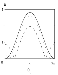
(b) The quantity $\mathcal{B}$ of Eq. (23) is shown vs $\theta_{u}$ for different values of $\lambda$. The other parameters are $\theta_{v}=\pi/4$, $\theta_{u^{\prime}}=-\pi/2$ and $\theta_{v^{\prime}}=-\pi/4$.

Figure 1: Example A (dashed line $\lambda=0.20$, dotted line $\lambda=0.54$, solid line $\lambda=0.96$)

5.2 Example B

As second example we consider the entangled superposition

$$|\psi\rangle=\frac{1}{\sqrt{2}}\left(|0\rangle_{1}|0\rangle_{2}+|n\rangle_{1}|n\rangle_{2}\right)\,.$$ (24)

Since $|0\rangle$ and $|n\rangle$ are orthogonal for $n\neq 0$, the state (24) resembles a spin triplet state. The corresponding Wigner function is

$$W(q_{1},p_{1},q_{2},p_{2}) = \frac{1}{2\pi^{2}}\biggl{(}1+\frac{2^{n}}{n!}{(q_{1}-ip_{1})}^{n}{(q_{2}-ip_{2})}^{n}+\biggr{.}$$

$$+ \frac{2^{n}}{n!}{(q_{1}+ip_{1})}^{n}{(q_{2}+ip_{2})}^{n}+$$

$$+ \biggl{.}L_{n}(2q^{2}_{1}+2p^{2}_{1})L_{n}(2q^{2}_{2}+2p^{2}_{2})\biggr{)}\,e^{-q^{2}_{1}-q^{2}_{2}-p^{2}_{1}-p^{2}_{2}}.$$

where $L_{n}$ indicates the Laguerre polynomial of order $n$. By means of Eqs. (5) and (5.2) we get the tomogram of the state under consideration

$$w(X_{1},\theta_{1},X_{2},\theta_{2}) = \frac{1}{2\pi}\biggl{(}1+\frac{H_{n}(X_{1})H_{n}(X_{2})}{2^{n-1}n!}\cos n(\theta_{1}-\theta_{2})+\biggr{.}$$ (26)

$$+ \biggl{.}\frac{H^{2}_{n}(X_{1})H^{2}_{n}(X_{2})}{2^{2n}{(n!)}^{2}}\biggr{)}e^{-X^{2}_{1}-X^{2}_{2}}.$$

where $H_{n}$ indicates the Hermite polynomial of order $n$. Using the position of Eqs. (6) we obtain probabilities $w_{\pm\pm}(\theta_{1},\theta_{2})$

$$w_{++}(\theta_{1},\theta_{2}) = w_{--}(\theta_{1},\theta_{2})=\frac{1}{4}+\frac{H^{2}_{n-1}(0)}{\pi 2^{n}n!}\cos n(\theta_{1}+\theta_{2}),$$ (27)

$$w_{+-}(\theta_{1},\theta_{2}) = w_{-+}(\theta_{1},\theta_{2})=\frac{1}{4}-\frac{H^{2}_{n-1}(0)}{\pi 2^{n}n!}\cos n(\theta_{1}+\theta_{2}).$$ (28)

In Fig. 2(a) we show the behavior of the $w_{++}$ vs $\theta_{1}+\theta_{2}$ for different values of $n$. Also in this case they never exceed the value $1/2$, thus the quantities $E$, in Eq. (11), will be always confined between $1$ and $-1$, and the Bell’s inequality (10) will be satisfied.

For the state (24), Eq. (16) becomes

$$\mathcal{E}({\bf u},{\bf v})=\left\{\begin{array}[]{ll}\cos(\theta_{u}-\theta_{v})&n=1,\\ \cos\theta_{u}\cos\theta_{v}&n>1.\end{array}\right.$$ (29)

Then, in Fig. 2(b) we show $\mathcal{B}$ for the case of $n=1$. The nonclassical character of the entangled state (24) becomes now manifest.

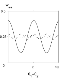
(a) The quantity $w_{++}(\theta_{1},\theta_{2})$ of Eq. (27) is shown vs $(\theta_{1}+\theta_{2})$ for different values of $n$ (dashed line $n=1$, dotted line $n=3$, solid line $n=5$).

(b) The quantity ${\cal B}$ derived from Eq. (29) is shown vs $\theta_{u}$ for case of $n=1$. The other parameters are $\theta_{v}=0$, $\theta_{u^{\prime}}=\pi$ and $\theta_{v^{\prime}}=\pi/2$.

Figure 2: Example B

5.3 Example C

As a third, and last, example we consider a pair-coherent state [26], namely

$$|\psi\rangle=N\int\limits^{2\pi}_{0}|re^{i\varphi}\rangle|re^{-i\varphi}\rangle\,d\varphi,$$ (30)

where norm $N$ is

$$N=\frac{e^{r^{2}}}{2\pi\sqrt{I_{0}(2r^{2})}}$$ (31)

with $I_{n}$ the modified Besssel function of order $n$. The state (30) represents two coherent states, of the same amplitude $r\in{\bf R}$, having a well defined phase relation although their own phase is random.

The Wigner function corresponding to the state (30) is

$$W(q_{1},p_{1},q_{2},p_{2})=\frac{N^{2}}{\pi^{2}}e^{-2r^{2}}\exp(-q^{2}_{1}-p^{2}_{1}-q^{2}_{2}-p^{2}_{2})\times$$ (32)

$$\times \int\limits^{2\pi}_{0}\int\limits^{2\pi}_{0}\exp\Bigl{(}\sqrt{2}r(q_{1}-ip_{1})(e^{i\varphi}+e^{-i\varphi^{\prime}})+\sqrt{2}r(q_{2}-ip_{2})(e^{-i\varphi}+e^{i\varphi^{\prime}})\Bigr{)}\times$$

$$\times \exp\Bigl{(}r^{2}[2\cos(\varphi-\varphi^{\prime})-\cos(2\varphi)-\cos(2\varphi^{\prime})]\Bigr{)}\,d\varphi\,d\varphi^{\prime}.$$

The tomogram of the state (30) is

$$w(X_{1},\theta_{1},X_{2},\theta_{2})=\frac{N^{2}}{\pi}e^{-2r^{2}}{|I(X_{1},\theta_{1},X_{2},\theta_{2})|}^{2}e^{-X^{2}_{1}-X^{2}_{2}},$$ (33)

where the integral $I(X_{1},\theta_{1},X_{2},\theta_{2})$ reads

$$I(X_{1},\theta_{1},X_{2},\theta_{2}) = \int\limits^{2\pi}_{0}\exp\Big{[}-\frac{r^{2}}{2}\left(e^{2i(\varphi-\theta_{1})}+e^{-2i(\varphi+\theta_{2})}\right)+\Big{.}$$ (34)

$$+ \Bigl{.}\sqrt{2}r\left(X_{1}e^{i(\varphi-\theta_{1})}+X_{2}e^{-i(\varphi+\theta_{2})}\right)\Big{]}\,d\varphi\,.$$

Using the procedure shown in the Appendix together with some algebra, we can obtain from Eq. (33) the following expressions for the probabilities $w_{\pm\pm}(\theta_{1},\theta_{2})$:

$$w_{\pm\pm}(\theta_{1},\theta_{2}) = \frac{N^{2}}{4}e^{-2r^{2}}\int\limits^{2\pi}_{0}\int\limits^{2\pi}_{0}\exp\Bigl{(}2r^{2}\cos(\varphi_{1}+\varphi_{2})\Bigr{)}\times$$

$$\times \left(1\mp{\rm erf}\left(\frac{r}{\sqrt{2}}\left[e^{i(\varphi_{1}-\varphi_{0})}+e^{i(\varphi_{2}+\varphi_{0})}\right]\right)\right)\times$$

$$\times \left(1\mp{\rm erf}\left(\frac{r}{\sqrt{2}}\left[e^{-i(\varphi_{1}+\varphi_{0})}+e^{-i(\varphi_{2}-\varphi_{0})}\right]\right)\right)\,d\varphi_{1}\,d\varphi_{2}\,,$$

where ${\rm erf}$ denotes the error function and $\varphi_{0}=(\theta_{1}+\theta_{2})/2$. Notice that the first (second) $\pm$ on the l.h.s. corresponds to the first (second) $\mp$ under the integral on the r.h.s.

The probabilities (5.3) are no longer bounded between the values $\{0,1/2\}$, thus, they can lead to violation of Bell’s inequalities. In particular, we show in Fig. 3(a) the dependence of $B$ from $r$ revealing violation of the CHSH inequality in a small range of the amplitude $r$. This result recall that of Ref. [9] where the state (30) was shown to violate another Bell’s inequality.

For the state (30), Eq. (16) becomes

$$\mathcal{E}({\bf u},{\bf v})=\cos\theta_{u}\cos\theta_{v}+r^{2}\left(1-\frac{J_{0}(2r^{2})}{I_{0}(2r^{2})}\right)\sin\theta_{u}\sin\theta_{v}\,,$$ (36)

where $J_{n}$ denotes the Bessel function of order $n$. Then, in Fig. 3(b) we show $\cal{B}$ for $r=1.05$. The violation of CHSH inequality becomes now more pronounced.

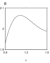
(a) The quantity $B$ derived from Eq. (5.3) is shown vs $r$ for parameters $\theta_{u}=\pi/2$, $\theta_{v}=-\pi/4$, $\theta_{u^{\prime}}=0$, $\theta_{v^{\prime}}-3\pi/4$.

(b) The quantity ${\cal B}$ derived from Eq. (36) is shown vs $\theta_{u}$ for parameters $r=1.05$, $\theta_{v}=0$, $\theta_{u^{\prime}}=\pi$, $\theta_{v^{\prime}}=\pi/2$.

Figure 3: Example C

6 Conclusions

In conclusions we have presented a tomographic approach to the quantum nonlocality of a bipartite continuous variable system. At first instance we have proposed a rough use of tomograms for testing violation of local hidden variable theory. In such a case one does not really need of a complete set of tomograms. However, the presence of purely quantum correlations are not easily recognizable. As matter of fact, the EPR state does not show the nonlocal character, while a pair-coherent state does.

Then, we have proposed to exploit the tomographically reconstructed state to get the statistics of pseudo-spin operators. This, practically, maps a continuous variable system into a discrete variable system making possible the use of standard Bell’s inequalities. This seeems a more powerful approach, but the price one ought to pay is the large amount of data (a complete set of tomograms) needed to reconstruct the state. In such a case the EPR state completely shows its nonlocal character. Also the pair-coherent state evidenciates much larger violations [27].

Our result opens possibilities for testing QM against local hidden variable theories using very efficient detection methods like homodyne detection [25].

Finally, the present approach could be straightforward extended to multipartite systems, e.g. making possible test of Grenberger-Horne-Zeilinger theorem [28] in continuous variables version [29]. Moreover, it could be useful to characterize quantum states used in information processing [5].

Appendix

By refering to Eq. (34) we note that the exponent of the imaginary argument is periodic, and since the integral is taken over a period of the exponent we can shift the angle argument as $\varphi-(\theta_{1}-\theta_{2})/2\to\varphi$ so the integral takes the form

$$I(X_{1},\theta_{1},X_{2},\theta_{2}) = \int\limits^{2\pi}_{0}\exp\Big{[}-\frac{r^{2}}{2}e^{-2i\varphi_{0}}\left(e^{2i\varphi}+e^{-2i\varphi}\right)+\Big{.}$$ (37)

$$+ \Big{.}\sqrt{2}re^{-i\varphi_{0}}\left(X_{1}e^{i\varphi}+X_{2}e^{-i\varphi}\right)\Big{]}\,d\varphi\,,$$

where we have set

$$\varphi_{0}=\frac{\theta_{1}+\theta_{2}}{2}\,.$$ (38)

Then, the integral can be rewritten as

$$I(X_{1},\theta_{1},X_{2},\theta_{2}) = \int\limits^{2\pi}_{0}\exp\left[-\frac{{(\alpha e^{i\varphi})}^{2}}{2}+\sqrt{2}\alpha e^{i\varphi}X_{1}\right]\times$$ (39)

$$\times \exp\left[-\frac{{(\alpha e^{-i\varphi})}^{2}}{2}+\sqrt{2}\alpha e^{-i\varphi}X_{2}\right]\,d\varphi\,,$$

where we have set

$$\alpha=re^{-i\varphi_{0}}\,.$$ (40)

Expanding each exponent in the above integral into a series of Hermite polynomials, and taking into account the equality

$$\int\limits^{2\pi}_{0}e^{i(n-m)\varphi}\,d\varphi=2\pi\delta_{n,m}\,,$$ (41)

we obtain the following expression

$$I(X_{1},\theta_{1},X_{2},\theta_{2})=2\pi\sum^{\infty}_{n=0}\frac{H_{n}(X_{1})H_{n}(X_{2})}{2^{n}{(n!)}^{2}}\alpha^{2n}\,.$$ (42)

Let us now consider two generic series

$$f(x_{1})=\sum\limits^{\infty}_{n=0}f_{n}x_{1}^{n}\quad{\rm and}\quad g(x_{2})=\sum\limits^{\infty}_{m=0}g_{m}x_{2}^{m}\,,$$ (43)

whose product yields

$$h(x_{1},x_{2})=f(x_{1})g(x_{2})=\sum^{\infty}_{n,m=0}f_{n}g_{m}x_{1}^{n}x_{2}^{m}\,.$$ (44)

How to express the sum of diagonal elements

$$s(x_{1},x_{2})=\sum^{\infty}_{n=0}f_{n}g_{n}x_{1}^{n}x_{2}^{n}$$ (45)

in terms of the $h(x_{1},x_{2})$ ? The answer is found by taking into account the equality (41), and it reads

$$s(x_{1},x_{2})=\frac{1}{2\pi}\int\limits^{2\pi}_{0}h\left(x_{1}e^{i\varphi},x_{2}e^{-i\varphi}\right)\,d\varphi\,.$$ (46)

The sum in right-hand side of Eq. (42) is the sum of diagonal terms of the product of two following series

$$f_{k}(\alpha)=\sum^{+\infty}_{n=0}\frac{H_{n}(X_{k})}{n!}{\left(\frac{\alpha}{\sqrt{2}}\right)}^{n}\quad k=1,2.$$ (47)

If we apply the formula (46) to this sum we obtain the representation (37) for it which we have started from. To obtain probabilities $w_{++}$ etc. we represent ${|I(X_{1},\theta_{1},X_{2},\theta_{2})|}^{2}$ in the following way:

$${|I|}^{2}=\int\limits^{2\pi}_{0}\int\limits^{2\pi}_{0}f_{1}(\alpha e^{i\varphi_{1}})f^{*}_{1}(\alpha e^{i\varphi_{1}})f_{2}(\alpha e^{i\varphi_{2}})f^{*}_{2}(\alpha e^{i\varphi_{2}})\,d\varphi_{1}\,d\varphi_{2}.$$ (48)

To calculate probability $w_{++}$ we need to take the following integral:

$$\int\limits^{2\pi}_{0}\int\limits^{2\pi}_{0}{|I(X_{1},\theta_{1},X_{2},\theta_{2})|}^{2}e^{-X^{2}_{1}-X^{2}_{2}}\,d\varphi_{1}\,d\varphi_{2},$$ (49)

and analogously for other probabilities. Swap integration order in these integrals we obtain the expression (5.3).

References

References

• [1] A. Einstein, B. Podolsky, N. Rosen, Phys. Rev. 47, 777 (1935).
• [2] J. S. Bell, Physics 1, 195 (1965); J. S. Bell, Speakable and Unspeakable in Quantum Mechanics, (Cambridge University Press, Cambridege, 1987).
• [3] A. Aspect, P. Grangier and G. Roger, Phys. Rev. Lett. 49, 91 (1982); A. Aspect, J. Dalibard and G. Roger, Phys. Rev. Lett. 49, 1804 (1982); Z. Y. Ou and L. Mandel, Phys. Rev. Lett. 61, 50 (1988); Y. H. Shih and C. O. Alley, Phys. Rev. Lett. 61, 2921 (1988); J. G. Rarity and P. R. Tapster, Phys. Rev. Lett. 64, 2495 (1990); J. Brendel, E. Mohler and W. Martienssen, Europhys. Lett. 20, 575 (1992); P. G. Kwiat, A. M. Steinberg and R. Y. Chiao, Phys. Rev. A 47, 2472 (1993); T. E. Kiess, Y. H. Shih, A. V. Sergienko and C. O. Alley, Phys. Rev. Lett. 71, 3893 (1993); P. G. Kwiat, K. Mattle, H. Weinfurter and A. Zeilinger, Phys. Rev. Lett. 75, 4337 (1995); D. V. Strekalov, T. B. Pittman, A. V. Sergienko, Y. Shih and P. G. Kwiat, Phys. Rev. A 54, 1 (1996).
• [4] D. Bohm, Quantum Theory, (Prentice Hall, Englewood Cliffs, NJ, 1951).
• [5] S. L. Braunstein and A. K. Pati, Quantum Information Theory with Continuous Variables, (Kluwer Academic Publishers, Dodrecht, 2001).
• [6] M. D. Reid and P. Drummond, Phys. Rev. Lett. 60, 2731 (1988); M. D. Reid, Phys. Rev. A 40, 913 (1989).
• [7] Z. Y. Ou, S. F. Pereira, H. J. Kimble and K. C. Peng, Phys. Rev. Lett. 68, 3663 (1992).
• [8] V. Giovannetti, S. Mancini and P. Tombesi, Europhys. Lett. 54, 559 (2001).
• [9] A. Gilchrist, P. Deruar and M. D. Reid, Phys. Rev. Lett. 80, 3169 (1998).
• [10] W. J. Munro and G. J. Milburn, Phys. Rev. Lett. 81, 4285 (1998).
• [11] J. Wenger, M. Hafezi, F. Grosshans, R. Tualle-Brouri and P. Grangier, Phys. Rev. A 67, 012105 (2003).
• [12] K. Banaszek and K. Wodkiewicz, Phys. Rev. A 58, 4345 (1998); K. Banaszek and K. Wodkiewicz, Phys. Rev. Lett. 82, 2009 (1999).
• [13] A. Kuzmich, I. A. Walmsley and L. Mandel, Phys. Rev. Lett. 85, 1349 (2000).
• [14] see e.g., Special Issue: Quantum State Preparation and Measurement, J. Mod. Opt. 44, N.11/12 (1997); D. G. Welsch, W. Vogel and T. Opatrny, Progress in Optics XXXIX, 63 (1999).
• [15] V. V. Andreev and V. I. Manko, J. Opt. B 2, 122 (2000).
• [16] H. Jeong, J. Lee and M. S. Kim, Phys. Rev. A 61, 052101 (2000).
• [17] S. L. Braunstein, A. Mann and M. Revzen, Phys. Rev. Lett. 68, 3259 (1992).
• [18] S. Mancini, V. I. Man’ko and P. Tombesi, Quantum and Semiclass. Opt. 7, 615 (1995); S. Mancini, V. I. Man’ko and P. Tombesi, Quantum and Semiclass. Opt. 9, 987 (1997).
• [19] S. Mancini, V. I. Man’ko and P. Tombesi, J. Mod. Opt. 44, 2281 (1997).
• [20] G. M. D’Ariano, U. Leonhardt and H. Paul, Phys. Rev. A 52 R1801 (1995).
• [21] G. M. D’Ariano, S. Mancini, V. I. Man’ko and P. Tombesi, Quantum and Semiclass. Opt. 8, 1017 (1996); M. G. Raymer, D. F. McAlister and U. Leonhardt, Phys. Rev. A 54, 2397 (1996).
• [22] J. F. Clauser, M. A. Horne, A. Shimony and R. A. Holt, Phys. Rev. Lett. 23 880 (1969).
• [23] L. Mista, R. Filip and J. Fiurasek, Phys. Rev. A 65, 062315 (2002); Z. B. Chen, J. W. Pan, G. Hou and Y. D. Zhang, Phys. Rev. Lett. 88, 040406 (2002).
• [24] V.V.Dodonov and V.I.Man’ko, Phys. Lett. A 229, 335 (1997).
• [25] D. F. Walls and G. J. Milburn, Quantum Optics, (Springer, Berlin, 1995).
• [26] G. Agarwal, Phys. Rev. Lett. 57, 827 (1986).
• [27] S. Mancini and P. Tombesi, Quant. Inf. and Comp. 3, 106 (2003).
• [28] D. M. Greenberger, M. A. Horne, A. Shimony and A. Zeilinger, Am. J. Phys. 58, 1131 (1990).
• [29] Z. B. Chen and Y. D. Zhang, Phys. Rev. A 65, 044102 (2002).