The non-Markovian stochastic Schrödinger equation for the position unraveling

Abstract

An important and well established area of quantum optics is the theory of Markovian stochastic Schrödinger equations (or by another name quantum trajectory theory). Recently stochastic Schrödinger equations have been developed for non-Markovian systems. In this paper we extend the current known stochastic Schrödinger equations for non-Markovian systems to include the position unraveling. We also discuss and illustrate that this stochastic Schrödinger equation can have an interpretation under both the orthodox and the de Broglie-Bohm hidden variable interpretation of quantum mechanics. We conclude that only the de Broglie-Bohm hidden variable theory provides a continuous-in-time interpretation of the non-Markovian stochastic Schrödinger equation.

I Introduction

In nature we are more likely to find a system interacting with an environment than isolated. Hence a common problem in physics (especially in the area of quantum optics) is to model open quantum systems Car93 . These systems consist of a small system (the system of interest) immersed in a lager system, which we refer to as the environment or bath. Due to the large Hilbert space of the bath it is convenient to describe the system by its reduced state. The reduced state is defined as

$$\rho_{\rm red}(t)={\rm Tr}_{\rm bath}[|{\Psi(t)}\rangle\langle{\Psi(t)}|],$$ (1)

where $|{\Psi(t)}\rangle$ is the combined system-bath state, found from the Schrödinger equation.

It has been shown Nak58 ; Zwa60 by a projection-operator method that we can write a general (non-Markovian) master equation for the reduced state as

$$d_{t}{\rho}_{\rm red}(t)=-\frac{i}{\hbar}[\hat{H}_{\rm int}(t),\rho_{\rm red}(t)]+\int_{t_{0}}^{t}\hat{\cal K}(t,s)\rho_{\rm red}(s)ds,$$ (2)

where $\hat{H}_{\rm int}(t)$ is a system operator in some interaction picture and $\hat{\cal K}(t,s)$ is the ‘memory time’ superoperator. It operators on the reduced state ${\rho}_{\rm red}(t)$ and represents how the bath affects the system. The problem with this equation is that in general the effect of $\hat{\cal K}(t,s)$ on ${\rho}_{\rm red}(t)$ can not be explicitly evaluated.

Recently non-Markovian stochastic Schrödinger equations (SSEs) DioGisStr98 ; StrDioGis99 ; GamWis02a ; GamWis02b ; Bud00 ; BasGhi02 ; Bas03 have been proposed which allow an alternative procedure for solving the reduced state. A non-Markovian SSEs is a stochastic equation for the system state $|{\psi_{z}({t})}\rangle$, conditioned on some noise function $z(t,s)$. (The double time argument in $z$ will be explained in Sec. III.) The SSE has the property that when the outer product of $|{\psi_{z}({t})}\rangle$ is averaged over all the possible $z(t,s)$ one obtains $\rho_{\rm red}$(t). That is,

$$\rho_{\rm red}(t)=E[|{\psi_{z}({t})}\rangle\langle{\psi_{z}({t})}|],$$ (3)

where $E[...]$ denotes an ensemble average over all possible $z(t,s)$’s.

When using non-Markovian SSEs to solve the reduced state it turns out that in general we can not explicitly evaluate $|{\psi_{z}({t})}\rangle$GamWis02b . That is, we can only explicitly write a non-Markovian SSE for situations where a reduced state can be found exactly be other means. However as shown in Ref. YuDioGisStr99 one can perform a post-Markov perturbation to the non-Markovian SSE, which allows approximate results for $\rho_{\rm red}(t)$ when the system is close to being Markovian. In Ref. GamWis02b we illustrated a different perturbation method that allows a perturbative result even when the system is strongly non-Markovian. However it is only valid for certain environment correlation functions (memory functions).

Here we are not interested in how to solve current non-Markovian SSEs. The aim of this paper is to firstly extend the known non-Markovian unravelings (different functional forms of $z(t,s)$) to include what we label the ‘position’ unraveling, and then secondly to outline a non-local hidden variable interpretation of this non-Markovian SSE. This hidden variable interpretation is similar to the de Broglie-Bohm interpretation of quantum mechanics deB30 ; Boh52 ; Hol93 . In other work we will supply a general hidden variable interpretation to include the coherent and quadrature unravelings GamWis03c . These unravelings are important to the quantum optics community as they have as their Markovian limit heterodyne and homodyne detection. The position unraveling which is presented here does not have a well defined Markovian limit.

II General dynamics for non-Markovian SSEs

The aim of this section is to outline the model used to develop non-Markovian SSEs. The results of this paper are only applicable to situations when the dynamics of the open quantum system can be described by the total Hamiltonian

$$\hat{H}_{\rm sys}(t)\otimes\hat{1}+\hat{1}\otimes\hat{H}_{\rm bath}+\hat{V},$$ (4)

where $\hat{H}_{\rm sys}(t)=\hat{H}_{\Omega}+\hat{H}(t)$ is the system Hamiltonian, and the bath is modelled by a collection of harmonic oscillators (for optical open quantum systems this corresponds to the electromagnetic field). In terms of dimensionless position ($\hat{X}_{k}$) and momentum ($\hat{Y}_{k}$) operators, the Hamiltonian for the bath is

$$\hat{H}_{\rm bath}=\sum_{k}^{K}\frac{\hbar\omega_{k}}{2}(\hat{X}_{k}^{2}+\hat{Y}_{k}^{2}),$$ (5)

where $K$ is the total number of modes in the bath. These dimensionless operators have the commutator $[\hat{X}_{j},\hat{Y}_{k}]=i\delta_{j,k}$.

The interaction Hamiltonian, $\hat{V}$ we assume is linear. By this we mean it has the form

$$\hat{V}=i\hbar\sum_{k}^{K}\Big{[}\hat{L}g^{*}_{k}\frac{(\hat{X}_{k}-i\hat{Y}_{k})}{\sqrt{2}}-\hat{L}^{\dagger}g_{k}\frac{(\hat{X}_{k}+i\hat{Y}_{k})}{\sqrt{2}}\Big{]},$$ (6)

where $g_{k}$ is the coupling strength of the $k^{\rm th}$ mode to the system.

For calculation purposes we define an interaction frame such that the fast dynamics placed on the state by the Hamiltonians $\hat{H}_{\Omega}$ and $\hat{H}_{\rm bath}$ is moved to the operators. The unitary operator for this transformation is

$$\hat{U}_{0}(t,t_{0})=e^{-i(\hat{H}_{\Omega}\otimes\hat{1}+\hat{1}\otimes\hat{H}_{\rm bath})(t-t_{0})/\hbar}.$$ (7)

This allows us to write the Schrödinger equation as

$$d_{t}|{{\Psi}(t)}\rangle=-\frac{i}{\hbar}[\hat{H}_{\rm int}(t)+\hat{V}_{\rm int}(t)]|{\Psi(t)}\rangle,$$ (8)

where $\hat{H}_{\rm int}(t)$ is $H(t)$ in the interaction frame and

$$\hat{V}_{\rm int}(t) = i\hbar\sum_{k}^{K}\Big{[}\hat{L}g_{k}^{*}e^{i\Omega_{k}(t-t_{0})}\frac{(\hat{X}_{k}-i\hat{Y}_{k})}{\sqrt{2}}$$ (9)

$$-\hat{L}^{\dagger}g_{k}e^{-i\Omega_{k}(t-t_{0})}\frac{(\hat{X}_{k}+i\hat{Y}_{k})}{\sqrt{2}}\Big{]},$$

with $\Omega_{k}=\omega_{k}-\Omega$. Here we have finally restricted the form of $\hat{H}_{\Omega}$ to be such that $\hat{L}$ in the interaction frame simply rotates in the complex plane at frequency $\Omega$. That is $\hat{L}_{\rm int}(t)=\hat{L}e^{-i\Omega(t-t_{0})}$.

III Deriving the position non-Markovian SSE

Under the orthodox view Per93 of quantum mechanics the quantum state upon measurement undergoes a change which is consistent with the measurement results. This change in state has been termed a ‘collapse’. Whether this collapse is a real physical event or represents an update in the observer’s knowledge will not be consider here. The central point is that under this view our observation causes the wavefunction for the state to collapse. The standard way to model this collapse is to use quantum measurement theory (QMT) BraKha92 .

III.1 Quantum Measurement Theory

In open quantum systems a measurement is usually performed on the bath rather than directly on the system. Due to the entanglement between the bath and the system the measurement on the bath results in an indirect measurement of the system. For the position unraveling the measurement performed (on the bath) is to measure the set of dimensionless position operators $\{\hat{X}_{k}\}$. To mathematically describe this measurement process we consider the $K$-observables

$$\{{X}_{k}\}=\{(\{x_{k}\},\hat{\pi}_{\{x_{k}\}}=|{\{x_{k}\}}\rangle\langle{\{x_{k}\}}|\otimes{1}_{\rm sys})\}.$$ (10)

Here the eigenvalues $\{x_{k}\}$ represent the actual results of the measurement and the eigenstate $|{\{x_{k}\}}\rangle$ is the multi-mode state the bath is projected into upon measurement. Because this theory is done in the interaction frame the measurement is not exactly a position measurement. It is position defined in the interaction (rotating) frame which in the Schrödinger picture (stationary frame) represents a measurement which cycles between position and momentum.

To find the state of the bath and the system after the measurement we decompose the projector into measurement operators, $\hat{M}_{\{x_{k}\}}$, by $\hat{\pi}_{\{x_{k}\}}=\hat{M}_{\{x_{k}\}}^{\dagger}\hat{M}_{\{x_{k}\}}$. With this measurement operator the combined state after a measurement at time $t$, which yielded results $\{x_{k}\}$ is

$$|{\Psi_{\{x_{k}\}}(t)}\rangle=\frac{\hat{M}_{\{x_{k}\}}|{\Psi(t)}\rangle}{\sqrt{P(\{x_{k}\},t)}},$$ (11)

where $P(\{x_{k}\},t)$ is the probability density and is defined by

$$P(\{x_{k}\},t)=\langle{\Psi(t)}|\hat{\pi}_{\{x_{k}\}}\otimes\hat{1}_{\rm sys}|{\Psi(t)}\rangle.$$ (12)

For the rank-one projector, $|{\{x_{k}\}}\rangle\langle{\{x_{k}\}}|$, the measurement operator which satisfies the above decomposition is $\hat{M}_{\{x_{k}\}}=|{\{n_{k}\}}\rangle\langle{\{x_{k}\}}|$, where $|{\{n_{k}\}}\rangle$ is arbitrary and is the state the bath is left in after the measurement. For most optical situations this will be a vacuum state $|{\{0_{k}\}}\rangle$ (as in optical measurement the detector usually absorbs the photon). This results in the combined state becoming $|{\Psi_{\{x_{k}\}}(t)}\rangle=|{\{0_{k}\}}\rangle|{\psi_{\{x_{k}\}}(t)}\rangle$, where $|{\psi_{\{x_{k}\}}(t)}\rangle$ is defined as

$$|{\psi_{\{x_{k}\}}(t)}\rangle=\frac{\langle\{x_{k}\}|{\Psi(t)}\rangle}{\sqrt{P(\{x_{k}\},t)}},$$ (13)

which we label a conditioned system state. This conditioned system state has the property that

$$\rho_{\rm red}(t)=\int{P(\{x_{k}\},t)}|{\psi_{\{x_{k}\}}(t)}\rangle\langle{\psi_{\{x_{k}\}}(t)}|d\{x_{k}\}.$$ (14)

If we consider $\{x_{k}\}$ to be a set of random variables $\{x_{k}(t)\}$ chosen from the distribution ${P(\{x_{k}\},t)}$ then we can rewrite the reduced state as

$$\rho_{\rm red}(t)=E[|{\psi_{\{x_{k}(t)\}}(t)}\rangle\langle{\psi_{\{x_{k}(t)\}}(t)}|],$$ (15)

where $E$ denotes an average over ${P(\{x_{k}\},t)}$. This is the requirement outlined in Sec. I for a solution to a SSE. This suggests that the time derivative of $|{\psi_{\{x_{k}(t)\}}(t)}\rangle$ will be a non-Markovian SSE. To calculate this we need to be able to generate a self consistent differential equation for $|{\psi_{\{x_{k}(t)\}}(t)}\rangle$. This is complicated and to simplify this procedure we introduce linear quantum measurement theory (LQMT).

III.2 Linear Quantum Measurement Theory

LQMT uses the same principles as QMT except we use an ostensible distribution, $\Lambda(\{x_{k}\})$, in place of the actual distribution GoeGra94 ; Wis96 . Using this distribution the linear conditional state is

$$|{\bar{\psi}_{\{x_{k}\}}(t)}\rangle=\frac{\langle\{x_{k}\}|{\Psi(t)}\rangle}{\sqrt{\Lambda(\{x_{k}\})}}.$$ (16)

The bar above this linear state signifies that the state is unnormalised. As before the reduced state can be written as

$$\rho_{\rm red}(t)=\int{\Lambda(\{x_{k}\})}|{\bar{\psi}_{\{x_{k}\}}(t)}\rangle\langle{\bar{\psi}_{\{x_{k}\}}(t)}|d\{x_{k}\}.$$ (17)

Thus $\rho_{\rm red}(t)=\bar{E}[|{\bar{\psi}_{\{x_{k}(t)\}}(t)}\rangle\langle{\bar{\psi}_{\{x_{k}(t)\}}(t)}|]$ where $\bar{E}$ denotes $\{x_{k}(t)\}$ is chosen from the ostensible distribution $\Lambda(\{x_{k}\})$. Because $\Lambda(\{x_{k}\})$ is time independent $\{x_{k}(t)\}=\{x_{k}(t_{0})\}$ for all $t$ and $d_{t}|{\bar{\psi}_{\{x_{k}\}}(t)}\rangle=\partial_{t}|{\bar{\psi}_{\{x_{k}\}}(t)}\rangle$.

Using Eq. (16) the time derivative of $|{\bar{\psi}_{\{x_{k}\}}(t)}\rangle$ becomes

$$\partial_{t}|{\bar{\psi}_{\{x_{k}\}}(t)}\rangle=\frac{\langle\{x_{k}\}|d_{t}|{\Psi(t)}\rangle}{\sqrt{\Lambda(\{x_{k}\})}}.$$ (18)

Substituting into this Eq. (8) and the Hamiltonian defined in Eq. (9) the differential equation for the linear system state becomes

$$\partial_{t}|{\bar{\psi}_{\{x_{k}\}}(t)}\rangle = \Big{[}-\frac{i}{\hbar}\hat{H}_{\rm int}(t)+\frac{\sum_{k}(\hat{L}g_{k}^{*}x_{k}e^{i\Omega_{k}(t-t_{0})}-\hat{L}^{\dagger}g_{k}x_{k}e^{-i\Omega_{k}(t-t_{0})}}{\sqrt{2}}\Big{]}|{\bar{\psi}_{\{x_{k}\}}(t)}\rangle$$ (19)

$$-\frac{\sum_{k}(\hat{L}g_{k}^{*}e^{i\Omega_{k}(t-t_{0})}+\hat{L}^{\dagger}g_{k}e^{-i\Omega_{k}(t-t_{0})})}{\sqrt{2}}\frac{\partial_{x_{k}}\langle\{x_{k}\}|{\Psi(t)}\rangle}{\sqrt{\Lambda(\{x_{k}\})}}.$$

Choosing the ostensible distribution to be

$$\Lambda(\{x_{k}\})=|\langle{\{x_{k}\}}|\{0_{k}\}\rangle|^{2}=\prod_{k}\frac{\exp(-x_{k}^{2})}{\sqrt{\pi}},$$ (20)

results in

$$\partial_{t}|{\bar{\psi}_{\{x_{k}\}}(t)}\rangle = \Big{[}-\frac{i}{\hbar}\hat{H}_{\rm int}(t)+\sum_{k}\hat{L}g_{k}^{*}x_{k}\sqrt{2}e^{i\Omega_{k}(t-t_{0})}-\frac{\sum_{k}(\hat{L}g_{k}^{*}e^{i\Omega_{k}(t-t_{0})}+\hat{L}^{\dagger}g_{k}e^{-i\Omega_{k}(t-t_{0})})}{\sqrt{2}}\partial_{x_{k}}\Big{]}|{\bar{\psi}_{\{x_{k}\}}(t)}\rangle.$$

Note this ostensible distribution was chosen for simplicity (it is equal to the real distribution at $t=t_{0}$).

To define a SSE from Eq. (III.2) we make the random variables substitution $x_{k}\rightarrow x_{k}(t)$. This transforms the linear state as $|{\bar{\psi}_{\{x_{k}\}}(t)}\rangle\rightarrow|{\bar{\psi}_{\{x_{k}(t)\}}(t)}\rangle$. For the linear SSE the random variable $x_{k}(t)$ must satisfy $\bar{E}[x_{k}(t)]=0$ and $\bar{E}[x_{k}(t)x_{l}(t)]=\delta_{k,l}/2$ for all $t$ (due to Eq. (20)). It can be still argued that, even with this substitution, this is not strictly a SSE as to solve this we must simultaneously solve for all possible $\{x_{k}(t)\}$ (due to the partial derivative in Eq. (III.2)). To make it a SSE we need to replace the derivatives by operators, but before we do this, to keep with past literature, it is convenient to define a noise function $z(t,s)$ as

$$z(t,s) = \sum_{k}g_{k}\sqrt{2}x_{k}(t)e^{-i\Omega_{k}(s-t_{0})},$$ (22)

With this definition we can define the following two bath-correlation function

$$\bar{E}[z(t,s)z^{*}(t,s^{\prime})] = \sum_{k,l}g_{k}g_{l}^{*}2e^{-i\Omega_{k}(s-t_{0})+i\Omega_{k}(s^{\prime}-t_{0})}\bar{E}[x_{k}(t)x_{l}(t)]$$ (23)

$$= \sum_{k}|g_{k}|^{2}e^{-i\Omega_{k}(s-^{\prime}s)}=\alpha(s-s^{\prime}),$$ (24)

$$\bar{E}[z(t,s)z(t,s^{\prime})] = \sum_{k}g_{k}^{2}e^{-i\Omega_{k}(s+s^{\prime}-2t_{0})}=\gamma(s+s^{\prime})$$ (25)

and the $K$ partial derivatives become

$$\partial_{x_{k}} = \int_{t_{0}}^{t}\Big{[}\delta_{z(t,s)}\frac{\delta z(t,s)}{\delta x_{k}(t)}ds+\delta_{z^{*}(t,s)}\frac{\delta z^{*}(t,s)}{\delta x_{k}(t)}ds\Big{]}$$ (26)

$$= \int_{t_{0}}^{t}\sqrt{2}\Big{[}\delta_{z(t,s)}g_{k}e^{-i\Omega_{k}(s-t_{0})}ds+\delta_{z^{*}(s)}g^{*}_{k}e^{i\Omega_{k}(s-t_{0})}ds\Big{]},$$

where $\delta_{z^{*}(t,s)}$ and $\delta_{z^{*}(t,s)}$ are functional derivatives. In terms of the noise function, Eq. (III.2) becomes

$$\partial_{t}|{\bar{\psi}_{z}(t)}\rangle = \Big{\{}-\frac{i}{\hbar}\hat{H}_{\rm int}(t)+\hat{L}z^{*}(t,t)-\hat{L}\int_{t_{0}}^{t}\Big{[}\alpha^{*}(t-s)\delta_{z(t,s)}+\gamma^{*}(t+s)\delta_{z^{*}(t,s)}\Big{]}ds-\hat{L}^{\dagger}\int_{t_{0}}^{t}\Big{[}\alpha(t-s)\delta_{z^{*}(t,s)}$$ (27)

$$+\gamma(t+s)\delta_{z(t,s)}\Big{]}ds\Big{\}}|{\bar{\psi}_{z}(t)}\rangle.$$

Assuming the initial combined state to be $|{\Psi(t_{0})}\rangle=|{\{0\}_{k}}\rangle|{\psi(t_{0})}\rangle$ it is easily shown that $|{\bar{\psi}_{z}(t_{0})}\rangle\equiv|{{\psi}(t_{0})}\rangle$ thus the functional derivative with respect to $z(t,s)$ in the above equation will always have zero contribution. That is, we can rewrite Eq. (27) as

$$\partial_{t}|{\bar{\psi}_{z}(t)}\rangle = \Big{\{}-\frac{i}{\hbar}\hat{H}_{\rm int}(t)+\hat{L}z^{*}(t,t)-\int_{t_{0}}^{t}\Big{[}\hat{L}\gamma^{*}(t+s)$$ (28)

$$+\hat{L}^{\dagger}\alpha(t-s)\Big{]}\delta_{z^{*}(t,s)}ds\Big{\}}|{\bar{\psi}_{z}(t)}\rangle.$$

This equation appears nicer than Eq. (III.2), but it is essentially the same equation and we still have the problem of representing the functional derivative by operators. To do this we make the two ansatzen,

$$\hat{A}_{z}(t)|{\bar{\psi}_{z}(t)}\rangle = \int_{0}^{t}ds\alpha(t-s)\delta_{z^{*}(t,s)}|{\bar{\psi}_{z}(t)}\rangle,$$ (29)

$$\hat{B}_{z}(t)|{\bar{\psi}_{z}(t)}\rangle = \int_{0}^{t}ds\gamma^{*}(t+s)\delta_{z^{*}(t,s)}|{\bar{\psi}_{z}(t)}\rangle.$$ (30)

With these ansatzen the linear non-Markovian SSE for the position unraveling is

$$\partial_{t}|{\bar{\psi}_{z}(t)}\rangle = \Big{\{}-\frac{i}{\hbar}\hat{H}_{\rm int}(t)+\hat{L}z^{*}(t,t)-\hat{L}\hat{B}_{z}(t)$$ (31)

$$-\hat{L}^{\dagger}\hat{A}_{z}(t)\Big{\}}|{\bar{\psi}_{z}(t)}\rangle.$$

In general these two ansatzen can not be solved, but as in coherent and quadrature unravelings GamWis02b ; YuDioGisStr99 there are perturbation techniques which could be extended to include this unraveling and would allow a perturbative solution. This we leave for later work.

III.3 The Non-Markovian SSE

In the above section we have presented the linear SSE for the position unraveling. To generate the actual non-Markovian SSE from this linear equation we have to first of all generate the set of random variable $\{x_{k}(t)\}$, which obey the real distribution $P(\{x_{k}\},t)$. These in general will be time dependent. To do this we use a Girsanov transformation GatGis91 ; DioGisStr98 to relate the real probability distribution with the ostensible one, that is

$$P(\{x_{k}\},t)=\Lambda(\{x_{k}\})\langle{\bar{\psi}_{\{x_{k}\}}(t)}|{\bar{\psi}_{\{x_{k}\}}(t)}\rangle.$$ (32)

Taking the time derivative of this and using Eq. (III.2) gives (after some manipulating)

$$d_{t}P(\{x_{k}\},t) = -\sum_{k}\partial_{x_{k}}\Big{\{}\langle{{\psi}_{\{x_{k}\}}(t)}|[\hat{L}g_{k}^{*}e^{i\Omega_{k}(t-t_{0})}$$ (33)

$$+\hat{L}^{\dagger}g_{k}e^{-i\Omega_{k}(t-t_{0})}]|{{\psi}_{\{x_{k}\}}(t)}\rangle$$

$$\times P(\{x_{k}\},t)\Big{\}}/\sqrt{2}.$$

This is effectively a drift equation for the probability density. It has associated with it the following set of differential equations

$$d_{t}x_{k}(t)={[\langle\hat{L}\rangle_{t}g_{k}^{*}e^{i\Omega_{k}(t-t_{0})}+\langle\hat{L}^{\dagger}\rangle_{t}g_{k}e^{-i\Omega_{k}(t-t_{0})}]}/{\sqrt{2}}$$ (34)

where $\langle\hat{L}\rangle_{t}=\langle{{\psi}_{\{x_{k}(t)\}}(t)}|\hat{L}|{{\psi}_{\{x_{k}(t)\}}(t)}\rangle$. Integrating this gives

$$x_{k}(t) = x_{k}(t_{0})+\int_{t_{0}}^{t}dt^{\prime}[\langle\hat{L}\rangle_{t^{\prime}}g_{k}^{*}e^{i\Omega_{k}(t^{\prime}-t_{0})}$$ (35)

$$+\langle\hat{L}^{\dagger}\rangle_{t^{\prime}}g_{k}e^{-i\Omega_{k}(t^{\prime}-t_{0})}]/{\sqrt{2}},$$

where $x_{k}(t_{0})$ is the random variable associated with the distribution $\langle{\Psi(t_{0})}|\hat{\pi}_{x_{k}}|{\Psi(t_{0})}\rangle$, which for an initial combined state of the form $|{\Psi(t_{0})}\rangle=|{\{0_{k}\}}\rangle|{\psi(t_{0})}\rangle$ is equivalent to the above ostensible distribution, Eq. (20). The noise function for the real distribution, defined in Eq. (22), becomes

$$z(t,s)=z(t_{0},s)+\int_{t_{0}}^{t}dt^{\prime}{[\langle\hat{L}\rangle_{t^{\prime}}\alpha(s-t^{\prime})+\langle\hat{L}^{\dagger}\rangle_{t^{\prime}}\gamma(s+t^{\prime})]}$$ (36)

where $z(t_{0},s)$ is equivalent to the noise function used in the linear non-Markovian SSE.

To generate the non-Markovian SSE we use Eqs. (13) and (16) to rewrite the conditioned state $|{{\psi}_{\{x_{k}(t)\}}(t)}\rangle=|{{\psi}_{\{x_{k}\}}(t)}\rangle|_{\{x_{k}=x_{k}(t)\}}$ as

$$|{{\psi}_{\{x_{k}(t)\}}(t)}\rangle=\frac{|{\bar{\psi}_{\{x_{k}(t)\}}(t)}\rangle}{\sqrt{\langle\bar{\psi}_{\{x_{k}(t)\}}(t)|{\bar{\psi}_{\{x_{k}(t)\}}(t)}\rangle}}.$$ (37)

As long as $\{x_{k}(t)\}$ in $|{\bar{\psi}_{\{x_{k}(t)\}}(t)}\rangle$ are the random variables associated with the real distribution, Eq. (35), this will obey the correct statistics defined in Eq. (15). Using Eq. (31) and the standard definition for a total time derivative gives the following SSE (after some manipulation)

$$d_{t}|{{\psi}_{z}(t)}\rangle = \Big{\{}-\frac{i}{\hbar}\hat{H}_{\rm int}(t)+(\hat{L}-\langle\hat{L}\rangle_{t})z^{*}(t)-(\hat{L}-\langle\hat{L}\rangle_{t})\hat{B}_{z}(t)+\langle(\hat{L}-\langle\hat{L}\rangle_{t})\hat{B}_{z}(t)\rangle_{t}-(\hat{L}^{\dagger}-\langle\hat{L}^{\dagger}\rangle_{t})\hat{A}_{z}(t)$$ (38)

$$+\langle(\hat{L}^{\dagger}-\langle\hat{L}^{\dagger}\rangle_{t})\hat{A}_{z}(t)\rangle_{t}\Big{\}}|{{\psi}_{z}(t)}\rangle,$$

where $|{{\psi}_{z}(t)}\rangle\equiv|{{\psi}_{\{x_{k}(t)\}}(t)}\rangle$. Here we have again used the above ansatzen to remove the partial derivatives with respect to $\{x_{k}\}$. Under the orthodox interpretation, the solution of this equation at time $t$ is the state of the system given that a measurement has been performed on the bath at that time and yielded results $\{x_{k}(t)\}$. Since this measurement would change the bath state, the future evolution of the system would not be the same as if the measurement had not been performed. In other words, the solutions at different times correspond to different physical situation. Thus the linking of these solutions to make a trajectory for the system state is a fiction.

IV SIMPLE APPLICATION

To illustrate that this is a correct unraveling for a non-Markovian open quantum system, in this section we apply this theory to a simple model. The model is a two level atom (TLA) coupled linearly to a single mode bath ($K=1$) with no detuning. To get an exact solution for comparison we first of all solve the total Schrödinger equation for the combined state. For this system the Schrödinger equation in the interaction frame is

$$|{\dot{\Psi}(t)}\rangle=(g^{*}\hat{\sigma}\hat{a}^{\dagger}-g\hat{\sigma}^{\dagger}\hat{a})|{\Psi(t)}\rangle$$ (39)

where $\hat{L}=\hat{\sigma}=|{b}\rangle\langle{e}|$ is the lowering operator for the TLA and $|{e}\rangle$ and $|{b}\rangle$ are the excited and ground states of the TLA. The combined state can be written in terms of photon number states and atomic states as

$$|{\Psi(t)}\rangle=\sum_{s=e,b}\sum_{n}c_{s,n}|{s}\rangle|{n}\rangle.$$ (40)

Substituting this into Eq. (39) and using the fact that since the bath state is initially in a vacuum state the only nonzero amplitudes are $c_{e,0}$, $c_{b,0}$ and $c_{b,1}$, we get the following solutions (with $t_{0}=0$)

$$c_{e,0}(t) = c_{e,0}(0)\cos[|g|(t-t_{0})],$$ (41)

$$c_{b,0}(t) = c_{b,0}(0),$$ (42)

$$c_{b,1}(t) = c_{e,0}(0)\sin[|g|(t-t_{0})]e^{-i\theta},$$ (43)

where $\theta$ is the argument of the complex coupling constant $g$. Thus the reduced state is simply

$$\rho_{\rm red}(t) = c^{2}_{e,o}(t_{0})\cos^{2}[|g|(t-t_{0})]|{e}\rangle\langle{e}|+\{c^{2}_{b,0}(t_{0})+c^{2}_{e,o}(t_{0})\sin^{2}[|g|(t-t_{0})]\}|{b}\rangle\langle{b}|$$ (44)

$$+[c_{e,o}(t_{0})c^{*}_{b,0}(t_{0})|{e}\rangle\langle{b}|+c^{*}_{e,o}(t_{0})c_{b,0}(t_{0})|{b}\rangle\langle{e}|]\cos[|g|(t-t_{0})].$$

The general non-Markovian SSE defined in Eq. (38) for this simple system becomes

$$d_{t}|{{\psi}_{z}(t)}\rangle = \Big{\{}(\hat{\sigma}-\langle\hat{\sigma}\rangle_{t})z^{*}(t)-(\hat{\sigma}-\langle\hat{\sigma}\rangle_{t})\hat{B}_{z}(t)+\langle(\hat{\sigma}-\langle\hat{\sigma}\rangle_{t})\hat{B}_{z}(t)\rangle_{t}-(\hat{\sigma}^{\dagger}-\langle\hat{\sigma}^{\dagger}\rangle_{t})\hat{A}_{z}(t)$$ (45)

$$+\langle(\hat{\sigma}^{\dagger}-\langle\hat{\sigma}^{\dagger}\rangle_{t})\hat{A}_{z}(t)\rangle_{t}\Big{\}}|{{\psi}_{z}(t)}\rangle,$$

where

$$z(t)=g\sqrt{2}x_{1}(t)$$ (46)

and

$$x_{1}(t)=x_{1}(t_{0})+\int_{t_{0}}^{t}dt^{\prime}(g^{*}\langle\hat{\sigma}\rangle_{t^{\prime}}+g\langle\hat{\sigma}^{\dagger}\rangle_{t^{\prime}})/\sqrt{2}.$$ (47)

The value of the random variable $x_{1}(t_{0})$ is determined by the initial distribution

$$P(x_{1},t_{0})=\Lambda(x_{1})=\frac{\exp(-x_{1}^{2})}{\sqrt{\pi}}.$$ (48)

To find functional form of the two operators $\hat{A}_{z}(t)$ and $\hat{B}_{z}(t)$ we use Eqs. (29) and (30) and assume

$$\delta_{z^{*}(s)}|{\bar{\psi}_{z}(t)}\rangle = f(t,s)\hat{\sigma}|{\bar{\psi}_{z}(t)}\rangle,$$ (49)

This results in $\hat{A}_{z}(t)={A}_{z}(t)\hat{\sigma}$, and $\hat{B}_{z}(t)={B}_{z}(t)\hat{\sigma}$, where

$${A}_{z}(t) = \int_{t_{0}}^{t}ds|g|^{2}f(t,s),$$ (50)

$${B}_{z}(t) = \int_{t_{0}}^{t}ds{g^{*}}^{2}f(t,s).$$ (51)

That is ${A}_{z}(t)$ and ${B}_{z}(t)$ are independent of the noise function for this example. Taking the time derivative of these equations gives

$$\dot{A}_{z}(t) = |g|^{2}+\int_{t_{0}}^{t}|g|^{2}\dot{f}(t,s)ds,$$ (52)

$$\dot{B}_{z}(t) = {g^{*}}^{2}+\int_{t_{0}}^{t}{g^{*}}^{2}\dot{f}(t,s)ds.$$ (53)

Here we have used the fact that $f(t,t)=1$ GamWis02a . To find the form of $\dot{f}(t,s)$ we firstly need to define the linear non-Markovian SSE for this system. It is

$$\partial_{t}|{\bar{\psi}_{z}(t)}\rangle=[\hat{\sigma}z^{*}(t)-{A}_{z}(t)\hat{\sigma}^{\dagger}\hat{\sigma}]|{\bar{\psi}_{z}(t)}\rangle,$$ (54)

where $z(t)=g\sqrt{2}x_{1}(t)$ with $x_{1}(t)$ in the linear case being defined to have a value given by $\Lambda(x_{1})$ [see Eq. (48)]. Secondly we use the following consistency conditions

$$\delta_{z^{*}(s)}\partial_{t}|{\bar{\psi}_{z}(t)}\rangle = \partial_{t}\delta_{z^{*}(s)}|{\bar{\psi}_{z}(t)}\rangle.$$ (55)

Substituting Eq. (54) and Eq. (49) into this equation gives the following differential equation

$$\dot{f}(t,s) = f(t,s){A}_{z}(t),$$ (56)

which when substituted into Eqs. (52) and (53) gives

$$\dot{A}_{z}(t) = |g|^{2}+{A}^{2}_{z}(t),$$ (57)

$$\dot{B}_{z}(t) = {g^{*}}^{2}+{B}_{z}(t){A}_{z}(t).$$ (58)

Solving this set of coupled differential equation with the initial conditions ${A}_{z}(t_{0})={B}_{z}(t_{0})=0$ gives ${A}_{z}(t)=|g|\tan[|g|(t-t_{0})]$, and ${B}_{z}(t)=e^{-i2\theta}|g|\tan[|g|(t-t_{0})]$. Thus Eq. (45) is now numerically solvable. An example solution for $|{\psi_{z}(t)}\rangle$ is shown in Fig 1. Here it is observed that unlike a Markov trajectory the evolution is smooth. This is because with only one bath mode the bath correlation time is non-zero. In this figure the quantum state is displayed in the Block representation, that is $x(t)=\langle\hat{\sigma}\rangle_{t}+\langle\hat{\sigma}^{\dagger}\rangle_{t}$, $y(t)=-i\langle\hat{\sigma}\rangle_{t}+i\langle\hat{\sigma}^{\dagger}\rangle_{t}$ and $z(t)=\langle\hat{\sigma}^{\dagger}\hat{\sigma}\rangle_{t}-\langle\hat{\sigma}\hat{\sigma}^{\dagger}\rangle_{t}$. To show that this equation does reproduce the reduced state, the difference between the ensemble average of 1000 trajectories and the reduced state, Eq. (44), is shown in Fig. 2. It is observed that the ensemble averages does reproduce the reduced state within statistical error.

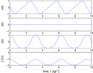
Figure 1: An example trajectory for the position non-Markovian SSE for a TLA in a single mode bath. Also shown is the real (solid) and imaginary (dotted) part of the noise function. Note the imaginary part for this system is equal to zero for all time. All calculations where done numerically with $g=1$, a time step size of 0.0001 and an excited state initial condition.

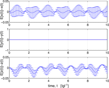
Figure 2: The difference between the ensemble average of 1000 trajectories for the position unraveling and the master equation for a TLA in a single mode bath. Other details are as in figure 1.

V A HIDDEN VARIABLE INTERPRETATION OF THE POSITION NON-MARKOVIAN SSE

In this section we present an alternative interpretation of the position non-Markovian SSE. The hidden variable interpretation we use is similar to the de Broglie-Bohm interpretation. The only difference is our position variables are ‘positions’ in a reference frame which rotates in phase space (the interaction frame). This results in our trajectories for the positions to be different from the standard de Broglie-Bohm trajectories deB30 ; Boh52 ; Hol93 . Moving to this frame simply means that the position states as we have defined them actual correspond to, in a stationary frame, a state which rotates between position and momentum. This is not a problem provided the Schrödinger equation used to develop the trajectories is in the interaction (rotating) frame.

In the standard de Broglie-Bohm theory, position has a reality prior to the measurement and its trajectory is deterministic assuming its initial position is known. To account for the weirdness of quantum mechanics its trajectory can be very non-classical. Specifically, the trajectory is influence by a extra potential, the quantum potential Boh52 ; Hol93 . This quantum potential depends on the solution of the Schrödinger equation, and is why the wavefunction is called the guiding wave deB30 ; Boh52 ; Hol93 . Thus under this interpretation the wavefunction is a real entity.

In this paper we will not be introducing the quantum potential as we can describe the trajectories with reference to only the wavefunction as a guiding wave. To mathematically describe this interpretation we use the fact that since the probability density is continuous in time and configuration space $\{x_{k}~{}\epsilon~{}\Re^{K}\}$ and is a conserved quantity, it must obey a continuity equation,

$$\partial_{t}P(\{x_{j}\},t)=-\sum_{k}\partial_{x_{k}}j_{k}(\{\ x_{j}\},t),$$ (59)

where $j_{k}(\{x_{j}\},t)$ is the current density and is related to the velocity field by $j_{k}(\{x_{j}\},t)=P(\{x_{j}\},t){\rm v}_{k}(\{x_{j}\},t)$. Each individual trajectory is then found by

$$d_{t}{x}_{k}(t)={\rm v}_{k}(\{x_{j}\},t)|_{\{x_{j}=x_{j}(t)\}}.$$ (60)

Thus to find this trajectory we need to know either ${\rm v}_{k}(\{x_{j}\},t)$ or $P(\{x_{j}\},t)$ and $j_{k}(\{x_{j}\},t)$. In previous literature the method is normally to find $P(\{x_{j}\},t)$ and $j_{k}(\{x_{j}\},t)$. Here, however, we propose that ${\rm v}_{k}(\{x_{j}\},t)$ is given by

$${\rm v}_{k}(\{x_{j}\},t)=\frac{{\rm Re}[\langle{\Psi(t)}|\{x_{j}\}\rangle\langle{\{x_{j}\}}|\hat{\rm v}_{k}(t)|{\Psi(t)}\rangle]}{\langle{\Psi(t)}|\{x_{j}\}\rangle\langle\{x_{j}\}|{\Psi(t)}\rangle},$$ (61)

where $\hat{\rm v}_{k}(t)$ is called the velocity operator. It is given by

$$\hat{\rm v}_{k}(t)=-\frac{i}{\hbar}[\hat{X}_{k},\hat{V}_{\rm int}(t)].$$ (62)

Note this is only valid for Hamiltonians with terms which are at most quadratic in $\hat{Y}$ (this is proven in Ref. GamWis03c ). This is not a problem as in nature all fundamental Hamiltonians are of this form.

Up until now we have not said anything about combined systems. If we now include an extra system, the system of interest, but only calculate trajectories for the bath positions, then the following differs slightly from the conventional de Broglie-Bohm theory. Defining the system state as

$$|{\psi_{\{x_{j}\}}(t)}\rangle=\frac{\langle{\{x_{j}\}}|\Psi(t)\rangle}{\sqrt{\langle\Psi(t)|{\{x_{j}\}}\rangle\langle{\{x_{j}\}}|\Psi(t)\rangle}},$$ (63)

the velocity field becomes

$${\rm v}_{k}(\{x_{j}\},t)={\rm Re}[\langle{\psi_{\{x_{j}\}}(t)}|\overrightarrow{\hat{\rm v}_{k}(\{x_{j}\},t)}|{\psi_{\{x_{j}\}}(t)}\rangle],$$ (64)

where

$$\overrightarrow{\hat{\rm v}_{k}(\{x_{j}\},t)}|{\psi_{\{x_{j}\}}(t)}\rangle=\frac{\langle{\{x_{j}\}}|\hat{\rm v}_{k}(t)|{\Psi(t)}\rangle}{\sqrt{\langle\Psi(t)|{\{x_{j}\}}\rangle\langle{\{x_{j}\}}|\Psi(t)\rangle}}.$$ (65)

Note the arrow defines the direction of operation [$\overrightarrow{\hat{\rm v}_{k}(\{x_{j}\},t)}$ will contain partial derivatives the act in the direction of the arrow]. Substituting the velocity field [Eq. (64)] into Eq. (60) results in following differential equation for the bath positions

$$d_{t}{x}_{k}(t)={\rm Re}[\langle{\psi_{\{x_{j}(t)\}}(t)}|\overrightarrow{\hat{v}_{k}(\{x_{j}(t)\},t)}|{\psi_{\{x_{j}(t)\}}(t)}\rangle],$$ (66)

where $|{\psi_{\{x_{j}(t)\}}(t)}\rangle=|{\psi_{\{x_{j}\}}(t)}\rangle|_{\{x_{j}=x_{j}(t)\}}$.

We now make the link that Eq. (63) is mathematically equivalent to Eq. (13) even though they have different physical interpretations. Since in Sec. III we showed that the position non-Markovian SSE is derived from this equation, then the time derivative of Eq. (63) must also give the correct non-Markovian SSE. Thus under this hidden variable interpretation the solution of the position non-Markovian SSE is a real entity which exists for all time and guides the trajectories for the bath positions $\{x_{k}(t)\}$. It gives the ‘conditioned’ system state at all times, as under the de Broglie-Bohm interpretation the bath positions exist even when we do not measure the bath.

To show that Eq. (66) does give the same trajectories as used in the non-Markovian SSE derived from QMT, we used the above definition for $\hat{\rm v}_{k}(t)$ and apply the Hamiltonians defined in Sec. II to them. This gives

$$\hat{\rm v}_{k}(t)=[g_{k}^{*}e^{i\Omega_{k}t}\hat{L}+g_{k}e^{-i\Omega_{k}t}\hat{L}^{\dagger}]/{\sqrt{2}},$$ (67)

which results in a velocity field of the form

$${\rm v}_{k}(\{x_{j}\},t) = [g_{k}^{*}e^{i\Omega_{k}t}\langle{\psi_{\{x_{j}\}}(t)}|\hat{L}|{\psi_{\{x_{j}\}}(t)}\rangle$$

$$+g_{k}e^{-i\Omega_{k}t}\langle{\psi_{\{x_{j}\}}(t)}|\hat{L}^{\dagger}|{\psi_{\{x_{j}\}}(t)}\rangle]/{\sqrt{2}}.$$

Thus the actual trajectories are found from

$$d_{t}x_{k}(t)={[\langle\hat{L}\rangle_{t}g_{k}^{*}e^{i\Omega_{k}t}+\langle\hat{L}^{\dagger}\rangle_{t}g_{k}e^{-i\Omega_{k}t}]}/{\sqrt{2}}$$ (69)

where $\langle\hat{L}\rangle_{t}=\langle{{\psi}_{\{x_{j}(t)\}}(t)}|\hat{L}|{{\psi}_{\{x_{j}(t)\}}(t)}\rangle$, which is the same as Eq. (34).

VI DISCUSSION AND CONCLUSION

In this paper we have firstly extended the theory of non-Markovian SSE to include the position unraveling. In Sec. IV we applied this theory to a simple system, a TLA coupled linearly to a single mode, to show that the position non-Markovian SSE does correctly average to give the reduced state. Although this unraveling does not have a well defined Markovian limit, it is still interesting to look at as it allows us to investigate interpretational questions in quantum mechanics. This is because this unraveling can be interpreted under either the orthodox interpretation or by a non-local hidden variable theory which is similar to the de Broglie-Bohm theory.

Under the orthodox theory the solution of the non-Markovian SSE at time $t$ is the state the system will be in if a measurement was performed on the bath at time $t$ and yielded results $\{x_{k}(t)\}$. Thus the non-Markovian SSE is simply a numerical tool for calculating the correct conditioned system state. In the de Broglie-Bohm hidden variable interpretation the non-Markovian SSE is an evolution equation for the system state (a real state) which guides the trajectories for the baths individual positions $\{x_{k}(t)\}$. Unlike the orthodox theory, these variables exist even when the bath is not measured. We conclude that if a non-trivial (non-numerical tool) interpretation is to be given to this non-Markovian SSE then we must consider the de Broglie-Bohm hidden variable interpretation of quantum mechanics.

- (1) H. J. Carmichael, An Open System Approach to Quantum Optics (Springer, Berlin, 19993).
- (2) S. Nakajima, “On quantum theory of transport phenomena,” Prog. Theor. Phys. 20, 948 (1958).
- (3) R. Zwanzig, “Ensemble method in the theory of irreversibility,” J. Chem. Phys. 33, 1338 (1960).
- (4) L. Diósi, N. Gisin, and W. T. Strunz, “Non-Markovian quantum state diffusion,” Phys. Rev. A 58, 1699 (1998).
- (5) W. T. Strunz, L. Diósi, and N. Gisin, “Open system dynamics with non-Markovian quantum trajectories,” Phys. Rev. Lett. 82, 1801 (1999).
- (6) J. Gambetta and H. M. Wiseman, “Non-Markovian Stochastic Schrödinger equations: generalization to real-valued noise using quantum measurement theory,” Phys. Rev. A 66, 012108 (2002).
- (7) J. Gambetta and H. M. Wiseman, “A perturbative approach to non-Markovian stochastic Schrödinger equations,” Phys. Rev. A 66, 052105 (2002).
- (8) A. A. Budini, “Non-Markovian Gaussian dissipative stochastic wave vector,” Phys. Rev. A 63, 012106, 2000.
- (9) A. Bassi and G. C. Ghirardi, “Dynamical reduction models with general Gaussian noises,” Phys. Rev. A 65, 042114 (2002).
- (10) A. Bassi, “Stochastic Schrödinger equations with general complex Gaussian noises,” Phys. Rev. A 67, 062101 (2003).
- (11) T. Yu, L. Diósi, N. Gisin, and W. T. Strunz, “Non-Markovian quantum state diffusion: perturbation approach,” Phys. Rev. A 60, 91 (1999).
- (12) A. Peres, Quantum theory: concepts and methods (Kluwer Academic, Boston, 1993).
- (13) L. de Broglie, An Introduction to the Study of Wave Mechanics, E. P. Dutton and company, Inc., New York, 1930.
- (14) D. Bohm, “A suggested interpretation of the quantum theory in terms of hidden variables, I & II”, Phys. Rev. 85, 166, 1952.
- (15) P. R. Holland, The quantum theory of motion: an account of the de Broglie- Bohm causal interpretation of quantum mechanics , Cambridge, Cambridge University Press, 1993.
- (16) J. Gambetta and H. M. Wiseman, “The interpretation of non-Markovian stochastic Schrödinger equations as a hidden variable theory,” Phys. Rev. A 68, 062104 (2003).
- (17) V.B. Braginsky and F.Y. Khalili, Quantum Measurement, Cambridge University Press, Cambridge, 1992.
- (18) P. Goetsch and R. Graham, “Linear stochastic wave equations for continuously measured quantum systems”, Phys. Rev. A 50, 5242 (1994).
- (19) H.M. Wiseman, “Quantum trajectories and quantum measurement theory”, Quantum Semiclass. Opt. 8, 205 (1996).
- (20) D. Gatarek and N. Gisin, “Continuous quantum jumps and infinite-dimensional stochastic equations,” J. Math. Phys. 32, 2152 (1991).
- (21) J. Gambetta and H. M. Wiseman, “Modal dynamics for non-orthogonal decompositions,” To be published in Found. Phys. (2003).