Remote preparation of quantum states

Abstract

Remote state preparation is the variant of quantum state teleportation in which the sender knows the quantum state to be communicated. The original paper introducing teleportation established minimal requirements for classical communication and entanglement but the corresponding limits for remote state preparation have remained unknown until now: previous work has shown, however, that it not only requires less classical communication but also gives rise to a trade–off between these two resources in the appropriate setting. We discuss this problem from first principles, including the various choices one may follow in the definitions of the actual resources.

Our main result is a general method of remote state preparation for arbitrary states of many qubits, at a cost of $1$ bit of classical communication and $1$ bit of entanglement per qubit sent. In this “universal” formulation, these ebit and cbit requirements are shown to be simultaneously optimal by exhibiting a dichotomy. Our protocol then yields the exact trade–off curve for memoryless sources of pure states (including the case of incomplete knowledge of the ensemble probabilities), based on the recently established quantum–classical trade–off for visible quantum data compression. A variation of that method allows us to solve the even more general problem of preparing entangled states between sender and receiver (i.e., purifications of mixed state ensembles).

The paper includes an extensive discussion of our results, including the impact of the choice of model on the resources, the topic of obliviousness, and an application to private quantum channels and quantum data hiding.

I Introduction

Teleportation Teleportation implements the transmission of a quantum bit ($1$ qubit) by sending two classical bits ($2$ cbits), while using up quantum correlation amounting to one bit of entanglement ($1$ ebit) – although a description of this state would require an infinite number of cbits, even when assisted by unlimited classical correlation. What is more, in teleportation this description is not needed at all: both the Sender and the Receiver act physically on the state (i.e. by quantum operations: completely positive and trace preserving linear maps), and the process can be used to transmit parts of entangled states faithfully. This and the phenomenon of dense coding Dense:coding prove that one cannot do with less than these resources: both $2$ cbits and $1$ ebit are necessary.

However, allowing the Sender knowledge of the state to be communicated changes the task to what is now known as remote state preparation (r.s.p.) Lo1999 ; Pati ; Zeng:Zhang , and here two new phenomena occur: in BDSSTW it is shown that at the cost of possibly spending more entanglement one can reduce the classical communication to $1$ cbit per qubit in the asymptotics; and there is a trade–off between the classical and the quantum resources needed, of which BDSSTW and Devetak:Berger provide bounds. In the present work we put these results into their definite form by proving a formula for the exact trade–off curve and by improving on the result of BDSSTW to use only $1$ cbit and $1$ ebit per qubit.

By a protocol for remote state preparation (r.s.p.) we shall mean a procedure involving two parties, a Sender who is given a description of a state $\rho\in{\cal X}\subset{\cal S}({\cal K})$ from a subset ${\cal X}$ of the state set ${\cal S}({\cal K})$ of the Hilbert space ${\cal K}$, and a Receiver who have access to a number of resources (both forward and backward classical communication, entanglement, shared randomness or others). The protocol prescribes how to use these in a sequence of steps (based on the previous exchange of messages in the protocol, and on $\rho$ for the Sender), resulting in a state $\widetilde{\rho}$ held by the Receiver. The dimension $D=\dim{\cal K}$ will, in the entire following discussion be the principal asymptotic parameter (i.e., one should think of it as large).

We shall say that the protocol is (deterministic) exact if $\widetilde{\rho}=\rho$ for all choices of $\rho\in{\cal X}$.

It is said to have fidelity $F$ if for all $\rho\in{\cal X}$, $F(\widetilde{\rho},\rho)\geq F$, with the mixed–state fidelity Uhlmann:fidelity ; Jozsa:fidelity $F(\rho,\sigma)=\|\sqrt{\rho}\sqrt{\sigma}\|_{1}^{2}={\operatorname{Tr}}\left(\sqrt{\sqrt{\rho}\sigma\sqrt{\rho}}\right)^{2}$. (Note that for $F=1$ this is the same as an exact protocol.)

A notion in between these two is a probabilistic exact protocol with error $\epsilon$: this means that the protocol additionally produces a flag, accessible to both Sender and Receiver, which indicates “success” or “failure” such that for all $\rho\in{\cal X}$, $\Pr\{\text{``failure''}\}\leq\epsilon$ and $\widetilde{\rho}=\rho$ if the flag is “success”; $\widetilde{\rho}$ is arbitrary otherwise. (Note that such a protocol automatically has fidelity $\geq 1-\epsilon$.)

Sometimes we want to impose a probability distribution $P$ on ${\cal X}$ and we will also consider protocols which have average fidelity $\overline{F}$, meaning

$$\int{\rm d}P(\rho)\,F(\widetilde{\rho},\rho)\geq\overline{F}.$$

Varied as the parameters by which we judge the quality of a protocol are, so are the ways to account for the use of resources: we will come back to this issue later (subsection VI.1), though the following example features not only various quality measures, but also some choices of resource accounting. For the moment we think only about protocols which terminate at a certain prescribed point and the resources are those needed to get to this point in the worst case $\rho\in{\cal X}$.

Example 1 (Column method BDSSTW )

The Sender is given an arbitrary pure state $\psi={{|{\psi}\rangle}\!{\langle{\psi}|}}$ (note that we use state synonymous with density operator; if we want to denote a state vector it will be ${|{\psi}\rangle}$) on a $D$–dimensional space (in BDSSTW $D=2^{n}$, i.e. $n$ qubits), and that Sender and Receiver share sufficiently many maximally entangled states ${|{\Phi_{D}}\rangle}=\frac{1}{\sqrt{D}}\sum_{j=1}^{D}{|{j}\rangle}{|{j}\rangle}$ of Schmidt rank $D$, labelled $1,2,\ldots,K$.

The Sender performs the measurement

$$\big{(}A_{0}=\overline{\psi},A_{1}={\openone}-\overline{\psi}\bigr{)}$$

on each of the $K$ entangled states and records the outcome. Here $\overline{\cdot}$ denotes the complex conjugation with respect to the basis $\{{|{j}\rangle}\}$ used to define $\Phi_{D}$. The probability of a $0$ clearly is $\frac{1}{D}$, the probability of a $1$ is $1-\frac{1}{D}$, hence the probability of $K$ $1$’s in a row (this will be called “failure”) is

$$\Pr\{\text{``failure''}\}=\left(1-\frac{1}{D}\right)^{K}\leq\exp\left(-\frac{K}{D}\right).$$

Thus, if $\log K\geq\log D+\log\log\frac{1}{\epsilon}$, “failure” occurs with probability at most $\epsilon$. If this does not happen, there is at least one $0$ in the measurement results, and it requires $\log K$ cbits to communicate the label of the entangled state where it occurred to the Receiver. For definiteness, let us say that the Sender selects one position of outcome $0$ at random. Simple algebra shows that in this case the Receiver’s reduced state is just $\psi$.

This is an example of a probabilistic exact protocol with asymptotic cost of classical communication of $1$ cbit per qubit and success probability $1-\epsilon$. By ignoring the possibility of failure, it becomes a fidelity $1-\epsilon$ protocol. The protocol requires $K\log D$ ebits, which is exponential in the number of qubits. Most of this however can be recovered (“recycled”) using back communication after completion of the remote state preparation (see BDSSTW ) such that only $O(\log D)$ ebits are irrecoverably lost.

Clearly, to make this method deterministic exact, one must not put a limit on the number of trials $K$ (in which case the communication cost becomes infinite), or we must allow for a deterministic exact procedure in the case of “failure”, e.g. teleportation. As this will increase the worst case communication cost to $2$ cbits per qubit, we are motivated to also consider expected cbit cost, which in this example is $1+2\epsilon$ per qubit.

As an aside to this exposition, one can also consider making the task easier for the Receiver, by only requiring that he is able to simulate any measurement of which he is given a description, performed on the state of which the Sender is given a description: this is known as classical teleportation CGM , and though it is related to our subject it lies outside the scope of the present paper.

The organisation of the rest of the paper is as follows: in section II we present a general method of remote state preparation, which uses $1$ cbit and $1$ ebit per qubit asymptotically. It is based on an efficient state randomisation method (see also PQC ). In section III it is shown that any universal high–fidelity protocol has to use $1$ cbit and $1$ ebit per qubit, asymptotically. The cbit bound is true even if unlimited quantum back communication is allowed, and the ebit bound is proved even in the presence of shared randomness. We proceed to derive the exact trade–off curve between ebits and cbits for an arbitrary ensemble of candidate states, in section IV, using the recently established analogous but simpler trade–off in quantum data compression between qubits and cbits HJW . Section V discusses the corresponding result if ensembles of pure entangled states between the Sender and the Receiver are to be prepared: again, we can prove the exact trade–off between ebits and cbits.

We conclude with a discussion of our findings and open questions in section VI: in particular considerations of the issue of obliviousness (cf. Leung:Shor ) and a discussion of the impact of certain slight changes in the model on our conclusions.

Several appendices contain separate or more technical issues: in appendix A facts about Gaussian distributed vectors are related; appendix B contains the proofs for the central technical result, the state randomisation; in appendix C it is shown that universal description of quantum states by qubits and cbits exhibits only a trivial trade–off between the resources: there is a dichotomy between full quantum with no classical information and no quantum with infinite classical information. Facts about typical subspaces, used in various proofs, are collected in appendix D. Appendix E contains thoughts on further operational links between the qubit/cbit and the ebit/cbit trade–off, based on a conjecture on the compressibility of mixed–state sources. Finally, in appendix F, miscellaneous proofs are collected.

Global notation conventions are: we use ^∗ for the Hermitian adjoint, ^⊤ for the transpose (in some given basis); $\exp$ and $\log$ are to basis $2$ (for the natural basis we use $e$, and the natural logarithm is denoted $\ln$).

II Universal r.s.p.:
1 cbit + 1 ebit $\mathbf{\succ}$ 1 qubit

We begin with a result on universal (approximate) state randomisation by unitaries:

Theorem 2

For Hilbert space ${\cal H}$ of dimension $D$ and $\epsilon>0$ there exist

$$K\leq\left(\frac{10}{\epsilon}\right)^{2}\!D\,\log\left(\frac{20D}{\epsilon}\right)$$

unitaries $U_{k}$ on ${\cal H}$ such that for every state $\varphi$,

$$\frac{1}{K}\sum_{k=1}^{K}U_{k}\varphi U_{k}^{*}\in\left[\frac{1-\epsilon}{D}{\openone};\frac{1+\epsilon}{D}{\openone}\right],$$ (1)

where the closed interval to the right refers to the operator order.

Proof . Select the unitaries independently at random from the Haar measure on the unitary group. Observe that eq. (1) says that for all pure states $\varphi$ and $\psi$,

$$\left|\frac{1}{K}\sum_{k=1}^{K}{\operatorname{Tr}}\bigl{(}U_{k}\varphi U_{k}^{*}\psi\bigr{)}-\frac{1}{D}\right|\leq\frac{\epsilon}{D}.$$

Fix a $\frac{\epsilon}{4D}$–net ${\cal M}$, according to lemma 4. Lemma 3 below allows us to bound

$$\begin{split}\Pr&\left\{\exists\varphi,\psi\!\in{\cal M}\ \left|\frac{1}{K}\sum_{k=1}^{K}{\operatorname{Tr}}\bigl{(}U_{k}\varphi U_{k}^{*}\psi\bigr{)}-\frac{1}{D}\right|>\frac{\epsilon}{2D}\right\}\\ &\phantom{=============:}\leq 2\left(\frac{20D}{\epsilon}\right)^{4D}\!\!\exp\left(-K\frac{\epsilon^{2}}{24}\right)\!.\end{split}$$

With triangle inequality for the trace norm we finally get

$$\begin{split}\Pr&\left\{\exists\varphi,\psi\ \left|\frac{1}{K}\sum_{k=1}^{K}{\operatorname{Tr}}\bigl{(}U_{k}\varphi U_{k}^{*}\psi\bigr{)}-\frac{1}{D}\right|>\frac{\epsilon}{D}\right\}\\ &\phantom{=============}\leq 2\left(\frac{20D}{\epsilon}\right)^{4D}\!\!\exp\left(-K\frac{\epsilon^{2}}{24}\right)\!,\end{split}$$

so if $K$ is as large as stated in the theorem there exist $U_{1},\ldots,U_{K}$ such that eq. (1) is true. $\Box$ The probabilistic and geometrical facts used in the above proof are contained in the following lemmas. The first is applied in the above proof with $p=1$ but the general version is used later on.

Lemma 3

Let $\varphi$ be a pure state, $P$ a rank $p$ projector and let $(U_{k})_{k=1}^{K}$ be an i.i.d. sequence of $U(D)$–valued random variables, distributed according to Haar measure. Then, for $0<\epsilon\leq 1$,

$$\begin{split}\Pr&\left\{\left|\frac{1}{K}\sum_{k=1}^{K}{\operatorname{Tr}}(U_{k}\varphi U_{k}^{*}P)-\frac{p}{D}\right|\geq\frac{\epsilon p}{D}\right\}\\ &\phantom{===============}\leq 2\exp\left(-Kp\frac{\epsilon^{2}}{6}\right).\end{split}$$

Proof . In appendix B. $\Box$

Lemma 4

Let ${\cal H}$ be a Hilbert space of dimension $D$. Then there exists, for every $\epsilon>0$, a set ${\cal M}$ of pure state vectors in ${\cal H}$ of cardinality

$$|{\cal M}|\leq\left(\frac{5}{\epsilon}\right)^{2D}$$

such that for every state vector ${|{\varphi}\rangle}\in{\cal H}$ there exists a state vector ${|{\psi}\rangle}\in{\cal M}$ such that

$$\bigl{\|}\varphi-\psi\bigr{\|}_{1}\leq 2\sqrt{1-F(\varphi,\psi)}\leq 2\bigl{\|}{|{\varphi}\rangle}-{|{\psi}\rangle}\bigr{\|}_{2}\leq\epsilon.$$

Such a set ${\cal M}$ we call $\epsilon$–net.

Proof . In appendix B. $\Box$ A few words of interpretation: it is known AMTdW ; boykin:roychowdhury that if $\epsilon=0$, one needs $K\geq D^{2}$, and this is tight as the example of the generalised Pauli (sometimes called Weyl) operators shows. We call a selection of unitaries as in the theorem “randomising”, because application of a randomly chosen $U_{k}$ results in an almost maximally mixed state. Clearly, this has cryptographic applications, an exploration of which is to be found in our separate paper PQC .

Let us now show how to use this result to build a remote state preparation protocol: first of all, given a pure state $\psi$, one can write down the family of operators

$$A_{k} =\frac{D}{K(1+\epsilon)}U_{k}\overline{\psi}U_{k}^{*}\quad(k=1,\ldots,K)$$

$$A_{\rm failure} ={\openone}-\sum_{k=1}^{K}A_{k}.$$

This is a POVM by virtue of theorem 2.

Protocol $\mathbf{\Pi}$ (Description of $\psi$ at the Sender):

1. The Sender measures the POVM $(A_{k})$ of the above description on her half of the entangled state $\Phi_{D}$. and announces the result (either “failure” or $k=1,\ldots,K$).

2. If the message received is not “failure”, say $k$, the Receiver applies the unitary $U_{k}^{\top}$ to his part of the state $\Phi_{D}$.

Theorem 5

The above protocol realises remote state preparation for an arbitrary state ${|{\psi}\rangle}\in{\cal K}$ exactly with a probability of failure of exactly $\frac{\epsilon}{1+\epsilon}\leq\epsilon$.

In particular, exact probabilistic r.s.p. with error $\epsilon$ is possible using

$$\log D+2\log\frac{10}{\epsilon}+\log\log\frac{20D}{\epsilon}$$ cbits

$$\text{and}\phantom{===========:}\log D$$ ebits.

Proof . It is straightforward to check that the protocol, in case it does not produce a failure, exactly prepares ${|{\psi}\rangle}$ at the Receiver.

For the probability assertions: the event $k$ of the POVM $(A_{k})$ is triggered with probability exactly $\frac{1}{K(1+\epsilon)}$. Hence the probability of failure is

$$1-K\frac{1}{K(1+\epsilon)}=1-\frac{1}{1+\epsilon}=\frac{\epsilon}{1+\epsilon}.$$

The remaining claims are easy consequences of this. $\Box$

Corollary 6

Probabilistic exact remote state preparation is possible with $1$ cbit and $1$ ebit per qubit, asymptotically. $\Box$

III Optimality of cbit and
ebit resources

We will now show that both $1$ ebit and $1$ cbit per qubit are necessary asymptotically for universal r.s.p. protocols with high fidelity. More precisely, we assume a protocol like our protocol $\Pi$ in section II, which takes as input the description of an arbitrary state $\psi$ on a $D$–dimensional space ${\cal K}$, uses an entangled state of Schmidt rank $S$, forward communication of one out of $K$ messages, such that the output states $\widetilde{\rho}$ have fidelity $F$ to the ideal $\psi$.

Regarding the communication resources, causality shows that $K\geq FD$ is necessary, even if unlimited quantum back communication is allowed: this is because the mere capability to remotely prepare an orthogonal basis of states with fidelity $F$ clearly allows the Sender to transmit one out of $D$ classical messages with probability at least $F$ of correct decoding. Imagine now that Sender and Receiver follow the r.s.p. protocol with the modification that each forward communication is skipped and replaced by the Receiver guessing it at random.

In this modification of the protocol, the probability of correct decoding clearly is $\geq\frac{F}{K}$, as the Receiver has only to guess the correct classical communication out of $K$. But the modified protocol involves no forward transmission at all, hence the probability of correctly identifying the Sender’s message — $1$ out of $D$ — is $\leq\frac{1}{D}$: this shows $\frac{1}{D}\geq\frac{F}{K}$.

We have thus proved:

Theorem 7

Any r.s.p. protocol with fidelity $F$ requires classical communication of

$$C=\log K\geq\log D+\log F\text{ cbits,}$$

even if unlimited quantum back communication is allowed. $\Box$

Regarding the entanglement, we have the following result of an extremely strong dichotomy:

Theorem 8

Any r.s.p. protocol using an entangled state of Schmidt rank $S\leq qD$ ($q<F$) requires classical communication of

$$C\geq\frac{q(1-q)}{6}D-O(\log D)\text{ cbits,}$$

even if unlimited shared randomness is available.

On the other hand, there is a protocol with fidelity $F\geq 1-\epsilon$, which uses no entanglement at all (i.e., $S=1$), and classical communication of

$$C\leq\left(4+\log\frac{1}{\epsilon}\right)D\text{ cbits.}$$

Thus, in the asymptotic limit, and with normalised resources $E=\log S/\log D$ and $R=C/\log D$ for the entanglement and communication rates, the rate point $E=1$ marks the threshold between two drastically different regimes: for $E\geq 1$, the classical communication rate $R=1$ is sufficient by corollary 6 and necessary by theorem 7. For any entanglement rate $E<1$, theorem 8 shows that no finite classical communication rate is possible: $R\rightarrow\infty$ with $D\rightarrow\infty$.

Thus, $E\geq 1$ and $R\geq 1$ hold simultaneously and both equalities can be achieved at the same time (theorem 5), unless $R=\infty$ in which case $E=0$. I.e., there is only a trivial trade–off between ebits and cbits.

Proof of theorem 8.  Consider any protocol, using a shared random variable $\nu$, so that the output state $\widetilde{\rho}$ is the mixture of the output states for the various values of $\nu$. Such a protocol clearly has average fidelity $\overline{F}\geq F$, with respect to the uniform (i.e., unitarily invariant) distribution on the pure states:

$$\overline{F}=\int{\rm d}{|{\psi}\rangle}\,F(\widetilde{\rho},{{|{\psi}\rangle}\!{\langle{\psi}|}}).$$

Because of the linearity of the pure state fidelity in $\widetilde{\rho}$, $\overline{F}$ is the probabilistic average of the fidelities $\overline{F}_{\nu}$ of the protocol for the value $\nu$ of the shared random variable. Hence there exists a $\nu$ such that $\overline{F}_{\nu}\geq F$, and we can consider a new protocol, without shared randomness, which has the same fidelity as the original.

Thus, w.l.o.g., we may assume a protocol of the form described in the first paragraph of this section, which uses only the entangled state $\Phi$ and forward classical communication. In general terms, it proceeds by the Sender performing a measurement on her half of $\Phi$ and communicating the outcome $m$ to the Receiver, who then applies a quantum operation $T_{m}$ to his half of $\Phi$. Observe that after the Sender’s measurement the state of the Receiver is collapsed to a state supported on the support of the restriction of $\Phi$, which is a space of dimension $S$. Thus, effectively, the Sender supplies the Receiver with a message $m$ and a state $\xi$ on an $S$–dimensional system, from the combination of which an approximation of $\psi$ is obtained: $\widetilde{\rho}=T_{m}(\xi)$. Once more using bilinearity of the pure state fidelity, we may assume that the choice of the pair $(m,\xi)$ from $\psi$ is deterministic, and that $\xi$ is a pure state. (This no longer describes an r.s.p. protocol, where uncontrollable randomness due to measurements is the rule: what is important here is that this can only enhance the capabilities of the Sender.)

We now invoke theorem 24 from appendix C, which lower bounds the classical communication cost of such a quantum–classical state description: we obtain

$$C\geq\frac{q(1-q)}{6}D-O(\log D),$$

which is our claim.

Conversely, in the situation with no entanglement, pick an $\sqrt{4\epsilon}$–net ${\cal M}$ of cardinality at most $\left(\frac{5}{2\sqrt{\epsilon}}\right)^{2D}$, according to lemma 4. Clearly, a valid protocol is this:

Given a state description of $\psi$, the Sender picks a ${|{\phi}\rangle}\in{\cal M}$ with fidelity $1-\epsilon$ (because lemma 4 is strong enough for that) to $\psi$, and sends the Receiver an identifier for $\phi$, which requires $\log|{\cal M}|$ cbits. $\Box$

IV Ensemble trade–off curve

While in the previous sections we considered universal r.s.p. (even though asymptotic, allowing any input state), in the present and following section we want to look at ensemble asymptotics: we consider an ensemble of quantum states ${\cal E}=\{{|{\psi_{i}}\rangle},p_{i}\}$ on the Hilbert space ${\cal H}$ of dimension $d$, and are interested in r.s.p. of the ensemble $\{{|{\psi_{I}}\rangle},p_{I}\}$ on ${\cal H}^{\otimes n}$, with states and probabilities

$${|{\psi_{I}}\rangle} ={|{\psi_{i_{1}}}\rangle}\otimes\cdots\otimes{|{\psi_{i_{n}}}\rangle},$$

$$p_{I} =p_{i_{1}}\cdots p_{i_{n}},$$

$$I =i_{1}\ldots i_{n},$$

and for large $n$. The notation for letters (lower case) and blocks (upper case) is used throughout this and the following section.

Note that even in the case that the ensemble contains all pure states on ${\cal H}$, the asymptotics will capture only the product states in ${\cal K}={\cal H}^{\otimes n}$, unlike the model of the previous sections.

We shall be interested in protocols which have average fidelity $\overline{F}$, i.e.,

$$\sum_{I}p_{I}{\operatorname{Tr}}\bigl{(}{{|{\psi_{I}}\rangle}\!{\langle{\psi_{I}}|}}\widetilde{\rho}_{I}\bigr{)}\geq\overline{F}.$$ (2)

By the monotonicity of the fidelity under partial traces, this implies the weaker condition

$$\sum_{I}p_{I}\frac{1}{n}\sum_{k=1}^{n}{\operatorname{Tr}}\bigl{(}{{|{\psi_{i_{k}}}\rangle}\!{\langle{\psi_{i_{k}}}|}}{\operatorname{Tr}}_{\neq k}\widetilde{\rho}_{I}\bigr{)}\geq\overline{F},$$ (3)

which we will find useful at times.

Note that by considering average fidelities as we do here, shared randomness becomes automatically useless, because we aim to prepare pure states with high fidelity (compare the proof of theorem 8).

On block–length $n$, a protocol for r.s.p. uses a maximally entangled state $\Phi_{D}$ of Schmidt rank $D$ shared between Sender (A) and Receiver (B). We consider here protocols which use only forward communication: their general form is described by a measurement POVM depending on $I$, ${\bf M}^{I}=(M^{I}_{j})_{j}$ with $j$ running over a set $\{1,\ldots,K\}$: after performing this POVM on her half of $\Phi_{D}$, the Sender communicates $j$, and the Receiver applies a quantum operation $T_{j}$ to his half of $\Phi_{D}$. We write $({\bf M},T)$ to denote such a protocol, sometimes adding a subscript $n$ to indicate the block–length.

The resources used are defined, in a way similar to HJW , as the entanglement rate

$${\operatorname{esupp}\,}({\bf M},T):=\frac{1}{n}\log D,$$

and the communication rate

$${\operatorname{csupp}\,}({\bf M},T):=\frac{1}{n}\log K.$$

(The notation is meant to remind one of “support”, since what we count here is the number of bits necessary to support the entanglement and the classical messages, respectively.) We say that a rate pair $(R,E)$ is achievable if for all $\epsilon,\delta>0$ there exists $n_{0}$ such that for all $n\geq n_{0}$ there are r.s.p. protocols $({\bf M},T)_{n}$ with fidelity $1-\epsilon$ and resources

$${\operatorname{csupp}\,}({\bf M},T) \leq R+\delta,$$

$${\operatorname{esupp}\,}({\bf M},T) \leq E+\delta.$$

This allows us to rigorously define the trade–off function $E^{*}$ by

$$E^{*}(R)=\min\{E|(R,E)\text{ is achievable}\}.$$

A similar trade–off is studied in HJW between cbits and transmitted qubits instead of ebits, which is a visible coding generalisation of the familiar Schumacher quantum data compression Schumacher ; Schumacher:Jozsa : such a protocol consists of a pair $(E_{n},D_{n})$ of encoding and decoding maps. The encoding takes $I$ to a combination of a quantum message supported on $n\,{\operatorname{qsupp}\,}(E_{n},D_{n})$ qubits and a classical message comprising $n\,{\operatorname{csupp}\,}(E_{n},D_{n})$ cbits, while the decoding is a quantum operation acting on these two, with the aim as before, to achieve a large average input–output fidelity.

Defining achievable rate pairs $(R,Q)$ analogous to the above, and letting

$$Q^{*}(R)=\min\{Q|(R,Q)\text{ is achievable}\},$$

we have the following single–letter formula for the quantum–classical trade–off (q.c.t.) curve:

Theorem 9 (Hayden, Jozsa and Winter HJW )

$$Q^{*}(R)=M({\cal E},R):=\min\left\{S(A:B|C)|S(A:C)\leq R\right\},$$ (4)

where the minimisation is over all tripartite states

$$\omega=\sum_{i}p_{i}{{|{i}\rangle}\!{\langle{i}|}}^{A}\otimes\psi_{i}^{B}\otimes\sum_{j}p(j|i){{|{j}\rangle}\!{\langle{j}|}}^{C},$$ (5)

for stochastic matrices $p(j|i)$; $j$ has a range of at most $m+1$ if the ensemble consists of $m$ states.

$$S(A:C) =S(A)+S(C)-S(AC)\text{ and}$$

$$S(A:B|C) =S(AC)+S(BC)-S(ABC)-S(C),$$

are the (conditional) quantum mutual information, defined via the von Neumann entropy $S$, referring implicitely to the state $\omega$: $S(AC)$ is the von Neumann entropy of $\omega$ restricted to $AC$, etc. $\Box$

In brief, once an optimal channel $p(j|i)$ is chosen, the scheme essentially works as sending part of the classical encoding $J=j_{1}\ldots j_{n}$ (only typical) using the Reverse Shannon Theorem BSST , and then Schumacher–compressing the induced “conditional” ensemble

$$\{\psi_{I},q(I|J) =q(i_{1}|j_{1})\cdots q(i_{n}|j_{n})\},\text{ with}$$

$$q(i|j) =\left(\sum_{i}p_{i}p(j|i)\right)^{-1}p_{i}p(j|i),$$

to its von Neumann entropy (note that the ensemble is a product of independent ensembles even though they are not all identical).

For each point $(R,Q)$ on the trade–off curve for the ensemble ${\cal E}$ we can, with the method of the previous section, construct an asymptotic and approximate r.s.p. protocol using $C=R+Q$ cbits and $E=Q$ ebits: We only have to use theorem 5 to remotely prepare the encoded state on $Q$ qubits, using $Q$ ebits and an additional $Q$ cbits, all per qubit.

We can summarise the finding as an upper bound on $E^{*}(R)$, in a strange implicit form:

$$E^{*}(R+Q^{*}(R))\leq Q^{*}(R).$$ (6)

Remark 10

Devetak and Berger Devetak:Berger happened to parametrise the q.c.t. curve for the uniform qubit ensemble. Using teleportation instead of our theorem 5 they obtained r.s.p. protocols using $C+2Q$ cbits and $Q$ ebits.

Using the chain rule $S(A:B|C)+S(A:C)=S(A:BC)$, we can put together theorem 9 and eq. (6) to obtain that

$$E^{*}(R)\leq\min\{S(A:B|C)|S(A:BC)\leq R\}.$$

In fact, we shall show in a moment that equality holds here:

Theorem 11

$$E^{*}(R)=N({\cal E},R):=\min\{S(A:B|C)|S(A:BC)\leq R\},$$ (7)

where the minimisation is over all tripartite states $\omega$ as in eq. (5).

Before we prove this, we state a little lemma collecting some properties of $N$:

Lemma 12

$N$ is convex, continuous and strictly decreasing in the interval where it takes finite positive values, which is $[S(B);S(A)]$. It obeys the following additivity relation for ensembles ${\cal E}_{1}$ and ${\cal E}_{2}$:

$$N({\cal E}_{1}\otimes{\cal E}_{2},R)=\min\bigl{\{}N({\cal E}_{1}\!,\!R_{1})+N({\cal E}_{2}\!,\!R_{2})|R_{1}+R_{2}\!=\!R\bigr{\}}\!.$$ (8)

Proof . In appendix F. $\Box$ Proof of theorem 11.  Only the direction “$\geq$” has to be proved: assume an r.s.p. protocol for block–length $n$ and with average fidelity

$$\overline{F}=\sum_{I}p_{I}{\operatorname{Tr}}\bigl{(}{{|{\psi_{I}}\rangle}\!{\langle{\psi_{I}}|}}\widetilde{\rho_{I}}\bigr{)}\geq 1-\epsilon.$$

Let us describe the protocol again: the Sender performs a measurement on her half of $n(E+\delta)$ EPR–pairs and sends the measurement result $j$ (obtained with probability $p(J|I)$ and collapsing the Receiver’s state to $\sigma_{I,j}$) to the Receiver (using $n(R+\delta)$ classical bits), who performs a quantum operation $T_{j}$ on his half of the EPR–pairs. The state thus produced is $\widetilde{\rho}_{I,j}$ and obviously $\widetilde{\rho}_{I}=\sum_{j}p(j|I)\widetilde{\rho}_{I,j}$.

Now, the post–measurement state, including a classical system $A$ to record $I$, can be written in the general form

$$\sigma=\sum_{I}p_{I}{{|{I}\rangle}\!{\langle{I}|}}^{A}\otimes\sum_{j}p(j|I)\sigma_{I,j}^{B}\otimes{{|{j}\rangle}\!{\langle{j}|}}^{C},$$

where $C$ is the classical system used for communicating $j$.

Entropic quantities of this state are related to the resources required by the protocol: first of all, $S_{\sigma}(A:BC)\leq n(R+\delta)$ because in total $n(R+\delta)$ bits are communicated, and their information cannot be exceeded by the information in what the receiver eventually gets, by causality. Similarly, because all the $\sigma_{I,j}^{B}$ are supported on the $nE$ qubits which form the Receiver’s half of the EPR–pairs, we get

$$n(E+\delta)\geq S_{\sigma}(B)\geq S_{\sigma}(B|C)\geq S_{\sigma}(A:B|C).$$

We may assume that the $T_{j}$ do not affect the system $C$, and because (conditional) mutual informations are non–increasing under local quantum operations, we obtain that

$$n(R+\delta) \geq S_{\widetilde{\rho}}(A:BC),$$ (9)

$$n(E+\delta) \geq S_{\widetilde{\rho}}(A:B|C),$$ (10)

with the state

$$\widetilde{\rho}=\sum_{I}p_{I}{{|{I}\rangle}\!{\langle{I}|}}^{A}\otimes\sum_{j}p(j|I)\widetilde{\rho}_{I,j}^{B}\otimes{{|{j}\rangle}\!{\langle{j}|}}^{C}.$$

(Note that $\widetilde{\rho}_{I,j}=T_{j}(\sigma_{I,j})$ for all $I,j$.) Our goal is now to switch in the latter expression to the ideal states ${{|{\psi_{I}}\rangle}\!{\langle{\psi_{I}}|}}$, arguing that we retain high fidelity to $\widetilde{\rho}$, and then invoking general continuity bounds for the entropy:

More precisely, define

$$\Omega=\sum_{I}p_{I}{{|{I}\rangle}\!{\langle{I}|}}^{A}\otimes\sum_{j}p(j|I){{|{\psi_{I}}\rangle}\!{\langle{\psi_{I}}|}}^{B}\otimes{{|{j}\rangle}\!{\langle{j}|}}^{C}.$$

Then we can estimate

$$\begin{split}\bigl{\|}\Omega-\widetilde{\rho}\bigr{\|}_{1}&=\sum_{I}p_{I}\sum_{j}p(j|I)\bigl{\|}{{|{\psi_{I}}\rangle}\!{\langle{\psi_{I}}|}}-\widetilde{\rho}_{I,j}\bigr{\|}_{1}\\ &\leq\sum_{I}p_{I}\sum_{j}p(j|I)2\sqrt{1-{\operatorname{Tr}}({{|{\psi_{I}}\rangle}\!{\langle{\psi_{I}}|}}\widetilde{\rho}_{I,j})}\\ &\leq\sum_{I}p_{I}2\sqrt{1-{\operatorname{Tr}}({{|{\psi_{I}}\rangle}\!{\langle{\psi_{I}}|}}\widetilde{\rho}_{I})}\\ &\leq 2\sqrt{1-\overline{F}}\leq 2\sqrt{\epsilon},\end{split}$$

where in the second line we have used the inequality $\frac{1}{2}\|\rho-\sigma\|_{1}\leq\sqrt{1-F(\rho,\sigma)}$ for states $\rho,\sigma$ Fuchs:vandeGraaf , and then concavity of the square root function. Because for states $\rho,\sigma$ on a $D$–dimensional system, $\|\rho-\sigma\|_{1}\leq\epsilon\leq\frac{1}{2}$, we have the Fannes inequality fannes $|S(\rho)-S(\sigma)|\leq-\epsilon\log\frac{\epsilon}{D}$, we obtain that there exists a function $f(\epsilon)$, vanishing as $\epsilon\rightarrow 0$, such that

$$n(R+\delta) \geq S_{\Omega}(A:BC)-nf(\epsilon),$$ (11)

$$n(E+\delta) \geq S_{\Omega}(A:B|C)-nf(\epsilon).$$ (12)

The reasoning is that the entropies of combinations of $A$, $B$ and $C$ relative to the states $\Omega$ and $\widetilde{\rho}$, see eqs. (9) and (10), can be estimated against each other by the Fannes inequality, observing that Hilbert space dimensions are of the form $X^{n}$ with a constant $X$.

Hence we get (letting $\delta^{\prime}=\delta+f(\epsilon)$)

$$\begin{split}n(E+\delta^{\prime})&\geq\min_{\Omega}\{S(A:B|C)|S(A:BC)\leq n(R+\delta^{\prime})\}\\ &=N\bigl{(}{\cal E}^{\otimes n},n(R+\delta^{\prime})\bigr{)}\end{split}$$

Now we invoke lemma 12 to estimate further,

$$\begin{split}E+\delta^{\prime}&\geq\frac{1}{n}N\bigl{(}{\cal E}^{\otimes n},n(R+\delta^{\prime})\bigr{)}\\ &=\min\left\{\frac{1}{n}\sum_{k=1}^{n}N({\cal E},R_{k})\left|\frac{1}{n}\sum_{k=1}^{n}R_{k}=R+\delta^{\prime}\right.\right\}\\ &\geq N({\cal E},R+\delta^{\prime}),\end{split}$$

the second line by eq. (8), the third by convexity of $N$. Using the continuity of $N$ with $\delta^{\prime}\rightarrow 0$ (which occurs with $\epsilon,\delta\rightarrow 0$), we arrive at $E\geq N({\cal E},R)$, as desired. $\Box$

Readers of HJW will notice the similarity of the proofs of the lower bounds in theorems 9 and 11. Given that for the upper bound we use an operational transformation of a q.c.t. protocol into an r.s.p. protocol, one may wonder if there is not a proof of the optimality of this reduction by an inverse reduction of an r.s.p. protocol to a q.c.t. protocol. We relate one such attempt in appendix E.

There are two generalisations of theorem 9 which we can transport to obtain more general versions of theorem 11: the first is to lift the restriction to discrete ensembles, which is not really necessary - it is shown in HJW by suitable approximation (using in fact the net lemma 4) that theorem 9 holds true for an arbitrary probability distribution $p$ on the pure states of ${\cal H}$. This shows automatically that theorem 11 also holds in the same form for general ensembles (in general with $\inf$ instead of $\min$).

The second concerns the so–called arbitrarily varying sources (AVS): an ensemble is generally taken to represent some partial knowledge about the states to be encountered, and this model allows us to fine–tune this to even less knowledge: an AVS is a family of probability distributions $p_{s}$, $s\in{\cal S}$ on the space of pure states, with the intention that at each time step each of the distributions $p_{s}$ can occur. One might want to think of an adversary choosing $s^{n}=s_{1}\ldots s_{n}$, thus presenting a given protocol with the distribution of states

$$p_{s^{n}}=p_{s_{1}}\otimes\cdots\otimes p_{s_{n}}.$$

A protocol (of either q.c.t. or r.s.p.) is said to have fidelity $\overline{F}$ if for all choices $s^{n}\in{\cal S}^{n}$,

$$\int{\rm d}p_{s^{n}}(\psi)F({{|{\psi}\rangle}\!{\langle{\psi}|}},\widetilde{\rho})\geq\overline{F},$$

where $\widetilde{\rho}$ is the output state on input $\psi$.

It turns out HJW that for q.c.t. there is still a trade–off in this case, and that $Q^{*}(R)$ is given by the trade–off for the worst–case ensemble distribution from the convex hull ${\bf P}={\rm conv}\{p_{s}|s\in{\cal S}\}$ of the $p_{s}$:

Theorem 13

For an AVS $\{p_{s}\}_{s\in{\cal S}}$, the q.c.t. trade–off curve is given by

$$Q^{*}(R)=\sup_{p\in{\bf P}}Q^{*}(p,R),$$

where $Q^{*}(p,R)$ is the trade–off of theorem 9 as a function of cbit rate $R$ and the ensemble distribution $p$, made explicit. $\Box$

This immediately implies, by the same reasoning, the corresponding theorem for remote state preparation:

Theorem 14

For an AVS $\{p_{s}\}_{s\in{\cal S}}$, the r.s.p. trade–off curve is given by

$$E^{*}(R)=\sup_{p\in{\bf P}}E^{*}(p,R),$$

where $E^{*}(p,R)$ is the trade–off of theorem 11 as a function of cbit rate $R$ and the ensemble distribution $p$, made explicit. $\Box$

In particular, dropping all restrictions, i.e. for the AVS with ${\bf P}=\{\text{all distributions}\}$ (which means that the adversary may pick an arbitrary product state for the protocol), we obtain the “ultimate” trade–off functions ${\bf Q}^{*}$ and ${\bf E}^{*}$: these govern the asymptotic qubit/cbit and ebit/cbit cost of compressing and remotely preparing blocks of arbitrary states. Because we know that $Q^{*}(R)$ for the uniform distribution dominates all other curves with fixed input distribution (HJW , theorem 6.1 and corollary 9.2), we have ${\bf Q}^{*}(R)=Q^{*}(R,\text{uniform})$ and hence ${\bf E}^{*}(R)=E^{*}(R,\text{uniform})$. For qubits we thus can plot ${\bf E}^{*}$ thanks to the results of Devetak and Berger Devetak:Berger (Fig. 1).

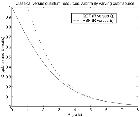
Figure 1: The q.c.t. trade–off curve for qubits vs. cbits according to Devetak and Berger Devetak:Berger (solid) and the implied r.s.p. trade–off for ebits vs. cbits (broken).

A word might be necessary to explain why there is no contradiction between this universal trade–off curve (which evidently exists not just for qubits, but for any qudits; to our knowlegde, however, it hasn’t been worked out explicitly for $d>2$), and the proof of the nonexistence of any finite trade–off in section III. This is because in the present section the task is much less ambitious: we only want to remotely prepare large blocks of (admittedly arbitrary) qubit states, i.e. a long product of pure states in small dimension. The set of product states however is much smaller than the set of all pure states on the large blocks. This fact is sufficient to allow an efficient trade–off between ebits (or qubits) and cbits.

V Preparation of entangled states

It is tempting to consider the generalisation of the previous section to mixed state sources. Observing however that our solution of the pure state case rested on the quantum–classical trade–off for pure state compression HJW — itself a generalisation of Schumacher’s source coding Schumacher — we might be discouraged by the corresponding mixed–state compression being far from resolved. A glimpse of this is provided in appendix E, but see a more detailed discussion in BCFJS ; Jozsa:Winter and references therein.

Instead, we target a seemingly harder problem: the Sender (A) should remotely prepare an entangled state between the Receiver (B) and herself, drawn from an ensemble. Clearly, the Receiver in this way obtains the mixed state ensemble of the reduced states.

In detail, assume an ensemble ${\cal E}=\{{|{\varphi_{i}}\rangle}^{AB},p_{i}\}_{i=1}^{m}$ of pure entangled states generating the i.i.d. source

$$I =i_{1}\ldots i_{n},$$

$${|{\varphi_{I}}\rangle} ={|{\varphi_{i_{1}}}\rangle}\otimes\cdots\otimes{|{\varphi_{i_{n}}}\rangle},$$

$$p_{I} =p_{i_{1}}\cdots p_{i_{n}}.$$

The protocols we consider are of a general form very similar to those in section IV: they allow both parties to use a maximally entangled state $\Phi_{D}$ of Schmidt rank $D$, and consist of a family of instruments davies:lewis ${\bf M}^{I}=(M_{j}^{I})_{j}$ ($j=1,\ldots,M$) for the Sender, i.e. each $M_{j}^{I}$ is a completely positive map, and their sum (over $j$) is a trace preserving map for every $I$ — this conveniently captures the notion of a (partial) measurement with a post–measurement state. Furthermore, there are quantum operations $T_{j}$ for the Receiver. The states prepared in this way are

$$\widetilde{\rho}_{I}=\sum_{j}(M_{j}^{I}\otimes T_{j})\Phi_{D},$$

and as before we demand that the fidelity $\overline{F}\geq 1-\epsilon$, with

$$\sum_{I}p_{I}{\operatorname{Tr}}\bigl{(}\varphi_{I}\widetilde{\rho}_{I}\bigr{)}\geq\overline{F}.$$

And similarly, we call a rate pair $(R,E)$ achievable if for all $\epsilon,\delta>0$ and sufficiently large $n$ there exist r.s.p. protocols with

$$\frac{1}{n}\log M \leq R+\delta,$$

$$\frac{1}{n}\log D \leq E+\delta.$$

Define the trade–off function for the ensemble ${\cal E}$,

$$E^{*}(R)=\min\{E|(R,E)\text{ achievable}\}.$$

We start by describing a protocol to achieve the rate point with the smallest $R$ allowed by causality (a different proof for the achievability of the cbit rate can be found in berry:sanders even though with a method that is very wasteful in terms of entanglement, much like the column method of example 1):

Proposition 15

There exists an r.s.p. protocol which achieves the rate pair

$$R =\chi\bigl{(}\{p_{i},\varphi_{i}^{B}\}\bigr{)},$$

$$E =S\left(\sum_{i}p_{i}\varphi_{i}^{B}\right),$$

with the Holevo quantity $\chi$ of the Receiver’s mixed state ensemble $\{p_{i},\varphi_{i}^{B}\}$.

Proof . Consider a string $I=i_{1}\ldots i_{n}$ of type (i.e. relative letter frequencies) $Q$ — see appendix D for details —, and construct (with $\delta>0$) the conditional typical projector $\Pi^{n}_{\varphi^{B}\!,\delta}(I)$ for $\varphi^{B}_{I}=\varphi^{B}_{i_{1}}\otimes\cdots\otimes\varphi^{B}_{i_{n}}$. By eq. (29), for sufficiently large $n$,

$${\operatorname{Tr}}\bigl{(}\varphi^{B}_{I}\Pi^{n}_{\varphi^{B}\!,\delta}(I)\bigr{)}\geq 1-\epsilon.$$

Construct also the typical projector $\Pi:=\Pi^{n}_{\rho,\delta}$ of the average state $\rho=\sum_{i}Q(i)\varphi^{B}_{i}$: by lemma 26, for sufficiently large $n$,

$${\operatorname{Tr}}\bigl{(}\varphi^{B}_{I}\Pi^{n}_{\rho,\delta}\bigr{)}\geq 1-\epsilon.$$

Hence, if we define (for all $I$ of type $Q$)

$$\pi_{I}:=\Pi^{n}_{\rho,\delta}\Pi^{n}_{\varphi^{B}\!,\delta}(I)\varphi^{B}_{I}\Pi^{n}_{\varphi^{B}\!,\delta}(I)\Pi^{n}_{\rho,\delta},$$

these operators have the properties

$${\operatorname{Tr}}\,\pi_{I} \geq 1-2\epsilon,$$ (13)

$$\pi_{I} \leq\exp\left(-n\bigl{(}S(\varphi^{B}|Q)-\delta\bigr{)}\right)\Pi^{n}_{\rho,\delta},$$ (14)

the latter is obtained by the definition of the conditional typical projector in appendix D; here, $S(\varphi^{B}|Q)=\sum_{i}Q(i)S(\varphi^{B}_{i})$.

Denoting the subspace onto which $\Pi^{n}_{\rho,\delta}$ projects by ${\cal T}$, its dimension, by eq. (27) is bounded

$$D:=\dim{\cal T}\leq\exp\left(n\bigl{(}S(\rho)+\delta\bigr{)}\right).$$ (15)

Now, for the Haar measure ${\rm d}U$ on the unitaries on ${\cal T}$,

$$\int{\rm d}U\,U\pi_{I}^{\top}U^{*}=({\operatorname{Tr}}\,\pi_{I})\frac{1}{D}\Pi.$$

Draw $U_{1},\ldots,U_{K}$ i.i.d. according to the Haar measure. Then, according to lemma 16 stated below,

$$\begin{split}\Pr&\left\{\frac{1}{K}\sum_{k}\frac{U_{k}\pi_{I}^{\top}U_{k}^{*}}{{\operatorname{Tr}}\pi_{I}}\not\in\frac{1}{D}[(1\pm\epsilon)\Pi]\right\}\\ &\phantom{===}\leq 2D\exp\left(-K\exp\bigl{(}-n(\chi+2\delta)\bigr{)}\frac{(1-2\epsilon)\epsilon^{2}}{2}\right),\end{split}$$

with $\chi=S(\rho)-S(\varphi^{B}|Q)$: because we can rescale the $\pi_{I}$ with the factor on the right hand side of eq. (14). Thus, by the union bound, there exist $U_{1},\ldots,U_{K}$ such that for all $I$ of type $Q$,

$$\frac{1-\epsilon}{D}\Pi\leq\frac{1}{K}\sum_{k}\frac{1}{{\operatorname{Tr}}\pi_{I}}U_{k}\pi_{I}^{\top}U_{k}^{*}\leq\frac{1+\epsilon}{D}\Pi,$$ (16)

if $K=(1+n\log m+\log D)\frac{2}{(1-2\epsilon)\epsilon^{2}}\exp\bigl{(}n(\chi+2\delta)\bigr{)}$.

The r.s.p. protocol now works as follows: the Sender, on getting $I$, determines its type $Q$ and sends it to the Receiver. If $\|p-Q\|_{1}>\delta$, the protocol aborts here (this happens with probability $\leq\epsilon$ if $n$ is sufficiently large, by the law of large numbers). For type $Q$ they have agreed on a list of unitaries $U_{1},\ldots,U_{K}$ as in eq. (16): the Sender can construct the measurement POVM

$$A_{k} =\frac{D}{K(1+\epsilon){\operatorname{Tr}}\pi_{I}}U_{k}\pi_{I}^{\top}U_{k}^{*},$$

$$A_{\rm failure} =\Pi-\sum_{k}A_{k},$$

and measures it (non–destructively) on the maximally entangled state $\Phi$ on ${\cal T}^{A}\otimes{\cal T}^{B}$. The outcome “${\rm failure}$” occurs with probability less than $\epsilon$, and in the case of outcome $k$ the Receiver, on learning the value $k$, can apply the unitary $U_{k}^{\top}$: it is straightforward to check that in this case he and the Sender share a purification of $\frac{1}{{\operatorname{Tr}}\pi_{I}}\pi_{I}$. Because of eq. (13) and the gentle measurement lemma 17 below, this state has high fidelity to $\varphi^{B}_{I}$, so by Uhlmann:fidelity ; Jozsa:fidelity she can apply a unitary to her post–measurement state to obtain a high–fidelity approximation of $\varphi^{AB}_{I}$.

Clearly, this protocol has a high average fidelity. In terms of resources, it requires a logarithmic number of bits to communicate the type $Q$ and

$$\log K\leq n\left(\chi\bigl{(}\{Q(i),\varphi_{i}^{B}\}\bigr{)}+f(\delta)\right)$$

to communicate the result of the measurement described above, with a function $f$ which vanishes as $\delta\rightarrow 0$. By eq. (15), it uses

$$\leq n\left(S\bigl{(}\sum_{i}Q(i)\varphi^{B}_{i}\bigr{)}+\delta\right)$$

ebits. With Fannes inequality fannes for $\|p-Q\|_{1}\leq\delta$, we obtain the claim. $\Box$

Lemma 16 (“Operator Chernoff bound” Ahlswede:Winter )

Let $X_{1},\ldots,X_{M}$ be i.i.d. random variables taking values in the operators ${\cal B}({\cal H})$ on the $D$–dimensional Hilbert space ${\cal H}$, $0\leq X_{j}\leq{\openone}$, with $A={\mathbbm{E}}X_{j}\geq\alpha{\openone}$, and let $0<\eta\leq 1/2$. Then

$$\begin{split}\Pr&\left\{\frac{1}{M}\sum_{j=1}^{M}X_{j}\not\in[(1-\eta)A;(1+\eta)A]\right\}\\ &\phantom{===============}\leq 2D\exp\left(-M\frac{\alpha\eta^{2}}{2\ln 2}\right).\end{split}$$

$\Box$

Lemma 17

For a state $\rho$ and an operator $0\leq X\leq{\openone}$, if ${\operatorname{Tr}}(\rho X)\geq 1-\epsilon$, then

$$\left\|\rho-\sqrt{X}\rho\sqrt{X}\right\|_{1}\leq\sqrt{8\epsilon}.$$

The main result of the present section is that this is essentially optimal:

Theorem 18

For the ensemble ${\cal E}=\{p_{i},\varphi_{i}\}$ of pure bipartite states and $R\geq 0$,

$$E^{*}(R)=N({\cal E},R):=\min\{S(B|C)\,|\,S(X:BC)\leq R\},$$

where the entropic quantities are with respect to the state $\omega$, and minimisation is over all $4$–partite states $\omega$ as follows:

$$\omega=\sum_{i}p_{i}{{|{i}\rangle}\!{\langle{i}|}}^{X}\otimes\varphi_{i}^{AB}\otimes\sum_{j}p(j|i){{|{j}\rangle}\!{\langle{j}|}}^{C},$$ (17)

with a classical channel $p(j|i)$.

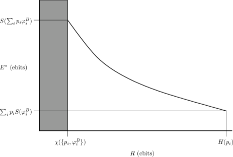
Figure 2: Schematic of the trade–off curve for an ensemble of entangled states. The shaded area is forbidden by causality and the curve begins at the point $\left(\chi\bigl{(}\{p_{i},\varphi_{i}^{B}\}\bigr{)},S\left(\sum_{i}p_{i}\varphi_{i}^{B}\right)\right)$, due to the protocol of proposition 15. It can never go below $E=\sum_{i}p_{i}S(\varphi_{i}^{B})$, which is reached at cbit rate $R=H(p)$, as this is the very amount of entanglement in the ensemble.

This theorem should be compared to the unentangled case, theorem 11, to which it provides a pleasingly direct generalisation. We see that despite the fact that the theorem applies to ensembles of entangled states, register $A$ does not appear in any of the entropic quantities involved. The trade–off curve is a function solely of the ensemble of mixed states at the Receiver. See Fig. 2 for a schematic view of the trade–off curve.

Before giving the proof, we state a crucial lemma (compare lemma 12), which we prove in appendix F:

Lemma 19

$N$ is convex, continuous and strictly decreasing in the interval $[S(X:B);S(X)]$. It obeys the following additivity relation for ensembles ${\cal E}_{1}$ and ${\cal E}_{2}$:

$$N({\cal E}_{1}\otimes{\cal E}_{2},R)=\min\bigl{\{}N({\cal E}_{1}\!,\!R_{1})+N({\cal E}_{2}\!,\!R_{2})|R_{1}+R_{2}\!=\!R\bigr{\}}\!.$$ (18)

$\Box$

Proof of theorem 18.  First, to show that, for fixed $R$, the pair $(R,N(R))$ is achievable, consider any channel $q(j|i)$, and let Sender and Receiver perform the following procedure (where all information quantities we encounter refer to the state $\omega$):

In step one, the channel $q^{n}$ is simulated (using shared randomness) on the typical $I$ by the Reverse Shannon Theorem BSST ; Jozsa:Winter , using $n\bigl{(}I(X:C)+\delta\bigr{)}$ of forward communication, within average total variational distance $\epsilon$ if $n$ is large enough.

Assuming that the channel $q^{n}$ is simulated ideally, we can proceed: with probability $1-\epsilon$, $J=j_{1}\ldots j_{n}$ is typical for the distribution $q_{j}=\sum_{i}p_{i}p(j|i)$, i.e. if ${\cal I}_{j}$ is the set of indices $i$ such that $j_{i}=j$, then

$$\forall j\quad\bigl{|}|{\cal I}_{j}|-nq_{j}\bigr{|}\leq\delta.$$

Now proposition 15 is used to remotely prepare the ensemble $\{q(i|j),\varphi_{i}\}$ on the block ${\cal I}_{j}$, with the conditional distribution

$$q(i|j)=\frac{1}{q_{j}}p_{i}p(j|i).$$

This requires

$$\leq n(q_{j}+\delta)\Bigl{(}\chi(\{q(i|j),\varphi^{B}_{i}\})+\delta\Bigr{)}\text{ cbits,}$$

$$\leq n(q_{j}+\delta)\Bigl{(}S\bigl{(}\sum_{i}q(i|j)\varphi^{B}_{i}\bigr{)}+\delta\Bigr{)}\text{ ebits.}$$

In total, we use $n\bigl{(}S(X:C)+S(X:B|C)+f(\delta)\bigr{)}$ cbits, and $n\bigl{(}S(B|C)+f(\delta)\bigr{)}$ ebits, and the average fidelity can be made arbitrarily close to $1$. Finally, the shared randomness can be disposed of, because the average fidelity is an average over it — hence there exists a value of the shared random variable such that the average fidelity is even larger.

Now for the converse direction, that $N$ is a lower bound: if $(R,E)$ is achievable, then for sufficiently large $n$ there exist protocols which use $n(R+\delta)$ cbits and $n(E+\delta)$ ebits, of fidelity $1-\epsilon$:

$$\sum_{I}p_{I}{\langle{\varphi_{I}}|}\widetilde{\rho}_{I}{|{\varphi_{I}}\rangle}\geq 1-\epsilon,$$

where $\widetilde{\rho}_{I}$ is the output state for input $I$. Any protocol has the following form: the Sender performs a measurement on her half of $n(E+\delta)$ EPR pairs, and then sends $n(R+\delta)$ bits of classical message $j$ to the Receiver. Conditioned on the classical message $j$, he then performs a decoding operation $T_{j}$ on his system. The outcome is a state $\widetilde{\rho}_{I,j}$ such that

$$\widetilde{\rho}_{I}=\sum_{j}p(j|I)\widetilde{\rho}_{I,j}.$$

The post–measurement state, including a classical system recording $I$, can be written in the form

$$\omega=\sum_{I}p_{I}{{|{I}\rangle}\!{\langle{I}|}}^{X}\otimes\omega_{I,j}^{AB}\otimes\sum_{j}p(j|I){{|{j}\rangle}\!{\langle{j}|}}^{C},$$

where system $C$ is communicated, and with $\widetilde{\rho}_{I,j}=T_{j}(\omega_{I,j})$. By causality, $S_{\omega}(X:BC)\leq n(R+\delta)$. Moreover, we can assume that the Receiver’s operation $T_{j}$ does not damage the $C$ register since the contents of the register could be copied prior to the application of $T_{j}$. Since $T_{j}$ cannot increase $S(X:BC)$ by data processing, however, we find that for the state

$$\widetilde{\rho}=\sum_{I}p_{I}{{|{I}\rangle}\!{\langle{I}|}}^{X}\otimes\widetilde{\rho}_{I,j}^{AB}\otimes\sum_{j}p(j|I){{|{j}\rangle}\!{\langle{j}|}}^{C},$$

the inequality

$$S_{\widetilde{\rho}}(X:BC)\leq n(R+\delta)$$

holds. Introducing

$$\Omega=\sum_{I}p_{I}{{|{I}\rangle}\!{\langle{I}|}}^{X}\otimes\varphi_{I}^{AB}\otimes\sum_{j}p(j|I){{|{j}\rangle}\!{\langle{j}|}}^{C},$$

we conclude that

$$S_{\Omega}(X:BC)\leq n(R+\delta+f(\epsilon)),$$ (19)

with some universal function $f$ vanishing with $\epsilon$: this is because of our fidelity assumption on the protocol and the bilinearity of the pure state fidelity, $F(\Omega,\widetilde{\rho})\geq 1-\epsilon$. (Compare the analogous computation in the proof of theorem 11.)

To bound the entanglement, observe that because the Sender’s measurement was on her half of $n(E+\delta)$ EPR pairs that the state $\omega_{j}^{B}=\sum_{I}q(I|j)\omega_{I,j}^{B}$ has support no larger than $2^{n(E+\delta)}$. (Note that $p_{I}p(j|I)$ defines a joint distribution on $I$ and $j$. We use $q(I|j)$ and $q_{j}$ to denote the associated conditional and marginal distributions.) Therefore, for the state $\omega_{XABC}$,

$$S_{\omega}(B|C)=\sum_{j}q_{j}S(\omega_{j}^{B})\leq n(E+\delta).$$

If Bob’s decoding operation $T_{j}$ were guaranteed to be unitary we could conclude $S_{\widetilde{\rho}}(B|C)\leq n(E+\delta)$. More generally, $T_{j}$ can be decomposed into three steps: adjoining an ancilla, applying a unitary and then tracing over the ancilla system. The first two steps leave the entropy invariant so without loss of generality, assume that conditioned on $j$, Sender and Receiver share a state $\omega_{I,j}^{ABB^{\prime}}$ and that $T_{j}={\operatorname{Tr}}_{B^{\prime}}$. Our strategy will be to use the fact that the states $\varphi_{I}^{AB}$ are pure to argue that the partial trace should not increase the entropy.

First, we now have $\omega_{I,j}^{AB}=\widetilde{\rho}_{I,j}^{AB}$. Let ${\langle{\varphi_{I}}|}\widetilde{\rho}_{I,j}{|{\varphi_{I}}\rangle}=1-\epsilon_{I,j}$. We can choose an extension $\varphi_{I}^{ABB^{\prime}}$ of $\varphi_{I}$ such that $F(\varphi_{I}^{ABB^{\prime}},\omega_{I,j}^{ABB^{\prime}})=1-\epsilon_{I,j}$ Jozsa:fidelity ; Uhlmann:fidelity . By the concavity of the fidelity, we then conclude that for

$$\varphi_{j} :=\sum_{I}q(I|j)\varphi_{I}^{ABB^{\prime}},$$

$$\omega_{j} :=\sum_{I}q(I|j)\omega_{I,j}^{ABB^{\prime}},$$

we have

$$F(\varphi_{j},\omega_{j})\geq\sum_{I}q(I|j)(1-\epsilon_{I,j})=:1-\epsilon_{j}.$$

Now, because $\varphi_{I}^{AB}$ is pure, the state $\varphi_{j}$ must be separable across the $AB-B^{\prime}$ cut. Therefore, $S(\varphi_{j}^{BB^{\prime}})\geq S(\varphi_{j}^{B})$. On the other hand, using the Fannes inequality and the concavity of its bound, we obtain

$$\begin{split}n(E+\delta)&\geq\sum_{j}q_{j}S(\omega_{j}^{BB^{\prime}})\\ &\geq\sum_{j}q_{j}\bigl{[}S(\varphi_{j}^{BB^{\prime}})-nf(\epsilon_{j})\bigr{]}\\ &\geq\sum_{j}q_{j}S(\varphi_{j}^{B})-nf(\epsilon),\end{split}$$

for some universal function $f$ vanishing with $\epsilon$. Hence,

$$S_{\Omega}(B|C)\leq n(E+\delta+f(\epsilon)).$$ (20)

Putting this together with eq. (19), we get, with $\delta^{\prime}=\delta+f(\epsilon)$ and the definition of $N$,

$$n(E+\delta^{\prime})\geq N\bigl{(}{\cal E}^{\otimes n},n(R+\delta^{\prime})\bigr{)}.$$

Now we can invoke lemma 19, and obtain

$$\begin{split}E+\delta^{\prime}&\geq\frac{1}{n}N\bigl{(}{\cal E}^{\otimes n},n(R+\delta^{\prime})\bigr{)}\\ &=\min\left\{\frac{1}{n}\sum_{k=1}^{n}N({\cal E},R_{k})\left|\frac{1}{n}\sum_{k=1}^{n}R_{k}=R+\delta^{\prime}\right.\right\}\\ &\geq N({\cal E},R+\delta^{\prime}).\end{split}$$

Finally, using continuity of $N$ in $R$, we obtain the result,

$$E\geq N({\cal E},R).$$

$\Box$

VI Discussion

In the following subsections we want to review what we have achieved, while pointing out open questions.

VI.1 Models and resources

In the introduction we have mentioned various subtly different ways to define remote state preparation (deterministic exact, probabilistic exact, high fidelity; see next subsection for oblivious), as well as ways to account for the resources used (worst case and expected cost).

Subsequently we have concentrated on probabilistic and high fidelity asymptotic protocols (for which worst case and expected cost coincide, as one can easily see). The justification of this choice is that it seems to be the one best suited to the asymptotic considerations at our focus.

However, as the following table shows, our conclusions are for the most part independent of the particulars of the model:

	Worst Case	Expected
Det. exact	?$\geq 1$ ebit, $2\geq$?$\geq 1$ cbits	$1$ ebit, $1$ cbit
Prob. exact	$1$ ebit, $1$ cbit
High fidelity	$1$ ebit, $1$ cbit
Oblivious	$1$ ebit, $2$ cbits
Approx. obl.	$1$ ebit, $1$ cbit

The entries “$1$ ebit, $1$ cbit” derive their achievability from our protocol $\Pi$ (theorem 5) — directly in the cases “Probabilistic exact”, “High fidelity” and “Approximately oblivious” (see the following subsection), and augmented by teleportation in the failure event for “Deterministic exact, Expected cost”. The upper bound “$1$ ebit, $2$ cbits” is of course teleportation, which indeed is oblivious (see the following subsection); that in the oblivious case $2$ cbits are indeed necessary was shown in Leung:Shor .

So, only the entry in the field “Deterministic exact, Worst case” is not entirely understood: in HHH:1:2 it is shown that an exact r.s.p. protocol for a single qubit requires at least $1$ ebit and $2$ cbits, just like teleportation. Whether the analogous statement for higher dimensions is true is unknown.

VI.2 Approximate obliviousness

An r.s.p. protocol is called oblivious to the Sender Leung:Shor if, like teleportation, it can be made into a quantum operation for her, which she can execute without knowing classically what state she is attempting to prepare. A protocol is called oblivious to the Receiver Leung:Shor if, again like teleportation, it leaks no information about the state being prepared beyond giving him a single specimen of it. In Leung:Shor it was shown that if a deterministic exact protocol for preparing states in dimension $D$ is oblivious to the Receiver, then it must be oblivious to the Sender also, and must therefore, like teleportation, use at least $\log D$ ebits and $2\log D$ cbits.

A similar penalty for receiver obliviousness exists even in a purely classical analog of r.s.p., namely the simulation of a noisy classical channel by noiseless forward classical communication (cbits) and shared randomness (rbits) between Sender and Receiver. The classical Reverse Shannon Theorem BSST gives a deterministic exact protocol for this task at an expected cbit cost approaching the simulated channel’s classical capacity $C$ in the limit of large block size, but it is not hard to show that for some channels any such exact efficient simulation must 1) have a worst-case cost exceeding its expected cost, and 2) must be non–oblivious to the Receiver. For example consider a binary symmetric channel with crossover probability $p$ and capacity $C=1+p\log p+(1-p)\log(1-p)$. Note that such a channel, given a block of $n$ inputs, has probability $P_{0}=(1-p)^{n}$ of transmitting the whole block exactly, without crossovers, and of course any exact simulation of the channel must simulate this rare event with the correct probability. But to avoid a violation of causality, the expected cost of the simulation, in instances where no crossover occurs in a block of size $n$, must be at least $n-\log(1/P_{0})$; otherwise, as in the column method, the Sender could use $\log(1/P_{0})+O(1)$ cbits of additional classical communication to designate a no–crossover instance within a general simulation, thereby communicating $n$ cbits about the input in less than $n$ cbits of forward communication. For $0<p<1/2$ the causality–imposed cost $n-\log(1/P_{0})=n(1+\log(1-p)$ exceeds the expected cost $nC$ of an efficient simulation according to the Reverse Shannon Theorem; therefore in any efficient exact simulation, 1) the worst case cost must be at least $n-\log(1/P_{0})$; and 2) the occurrence of a cost exceeding the expected cost $nC$ must be negatively correlated with the number of crossovers, leaking extra information about the channel input besides that contained in the correctly simulated output.

Resuming our discussion of obliviousness in r.s.p., we observe that the previously studied notions of obliviousness to the Receiver are exact, requiring that the protocol leak no information whatever about the input. In the present paper’s main context of approximate simulations it is more appropriate to use a more robust notion of approximate obliviousness:

Definition 20

An r.s.p. protocol for a set ${\bf X}$ of states on ${\cal K}$ is said to be approximate and approximately oblivious with parameters $(\epsilon,\delta)$ if

1. For all $\sigma\in{\bf X}$, if the Receiver’s output state is denoted $\rho^{B}$: $\frac{1}{2}\|\sigma-\rho^{B}\|_{1}\leq\epsilon$.

2. There exists a c.p.t.p. map $T$ on the Receiver’s system that maps his output state $\rho^{B}$ to a close approximation of the whole of what he gets from the protocol: the pre–image of $\rho^{B}$ (under his decoding operation), possible residual quantum states, and the classical messages. I.e.,

   $$\frac{1}{2}\|\{\text{Receiver's record}\}-T(\rho^{B})\|_{1}\leq\delta.$$

Note that our notion of “approximate obliviousness” does not arise from some a priori concept of what the Receiver must not learn. It is rather modelled after “zero–knowledge” in zero–knowledge proofs: the verifier gets nothing that he could not have simulated himself (see ZK-Proofs and subsequent literature).

Note that for $\epsilon=\delta=0$ we recover the definition of Leung:Shor of a deterministic exact and exactly oblivious protocol. It would be natural to conjecture that a robust version of the main result of Leung:Shor should hold:

For an approximate and approximately oblivious r.s.p. protocol with parameters $(\epsilon,\delta)$ (for the set ${\bf X}={\cal P}({\cal K})$ of all pure states on ${\cal K}$), the communication cost is $\geq 2-f(\epsilon,\delta)$ cbits per qubit, and it has to use $\geq 1-f(\epsilon,\delta)$ ebits per qubit. There, $f$ is a function that vanishes with $\epsilon,\delta\rightarrow 0$.

Instead, it turns out that our protocol $\Pi$ is indeed approximate and approximately oblivious in the sense of definition 20, with parameters $(\epsilon,\epsilon)$:

Clearly, part (1) of the definition is satisfied (we remove the failure event by having the Sender choose one uniformly distributed from the “good” messages in the case of a “failure”). Part (2) also is easily seen to be true: the simulating map is simply

$$T:{{|{\psi}\rangle}\!{\langle{\psi}|}}\longmapsto\sum_{k=1}^{K}\frac{1}{K}{{|{k}\rangle}\!{\langle{k}|}}\otimes\overline{U_{k}}{{|{\psi}\rangle}\!{\langle{\psi}|}}U_{k}^{\top}.$$

As an aside, we may return to the column–method, presented in example 1 (without recycling of entanglement): it is not hard to see that in fact also this procedure is approximate and approximately oblivious. Indeed, to simulate the Receiver’s view of the protocol, he only has to create an arbitrary state, say $\left(\frac{1}{D}{\openone}\right)^{\otimes K}$ and an arbitrary classical message (say, uniformly distributed) with probability $\epsilon$: this is to simulate the failure. With probability $\frac{1-\epsilon}{K}$ each, he generates the states

$$\left(\frac{1}{D}{\openone}\right)^{\otimes(k-1)}\otimes{{|{\psi}\rangle}\!{\langle{\psi}|}}\otimes\left(\frac{1}{D}{\openone}\right)^{\otimes(K-k)},$$

and the classical message $k=1,\ldots,K$. It is easily seen that this is $\epsilon$–close to the Receiver’s actual view.

VI.3 Further applications of randomisation
and trade–off r.s.p.

The remote state preparation of state ensembles turns out to have applications to other problems, which we simply list here for reference:

1. The protocol we described in section V for optimal preparation of pure entangled states produces, when one ignores the Sender’s half of the state, mixed states at the Receiver’s system with a classical communication cost exactly equal to the Holevo quantity of his ensemble. This result is in fact the Quantum Reverse Shannon Theorem QRST for cq–channels, and follows also from the alternative protocol described in berry:sanders .

2. Optimal remote state preparation of entangled states (section V) is invoked to prove capacity formulas and bounds for the classical communication capacity of bipartite unitaries assisted by unlimited or bounded entanglement BHLS ; harrow .

3. At the heart of our r.s.p. protocol is the state randomisation by relatively few unitaries (theorem 2). In fact, similar to previously considered private quantum channels AMTdW ; boykin:roychowdhury we obtain a private channel scheme, but with halved key length! By applying the randomisation to half of an entangled state, one even obtains very efficient schemes for data hiding in bipartite quantum states DLT ; DHT . Our separate paper PQC is devoted to an exploration of these applications.

Appendix A Gaussian distributed vectors

This appendix is largely a compilation of known facts about the distribution of random vectors following a Gaussian law, and of some of their moments: we freely use textbook knowledge of probability theory (see e.g. feller ), as well as parts of the treatment of large deviation theory by Dembo and Zeitouni Dembo:Zeitouni .

Recall that the Gaussian (or normal) distribution on the reals with mean $\mu$ and variance $\sigma^{2}$, denoted $N(\mu,\sigma^{2})$, is defined by the density

$$N(\mu,\sigma^{2})\{{\rm d}t\}=\frac{1}{\sqrt{2\pi\sigma^{2}}}e^{-\frac{(t-\mu)^{2}}{2\sigma^{2}}}{\rm d}t.$$

We shall phrase most of the following in terms of random variables. That a random variable $X$ is distributed according to some Gaussian is denoted $X\sim N(\mu,\sigma^{2})$.

Definition 21

A Gaussian complex number with mean $\mu\in{\mathbbm{C}}$ and variance $\sigma^{2}>0$ is a random variable $\gamma=X+iY$, where $X$ and $Y$ are independent real random variables with $X\sim N\!\left({\rm Re}\,\mu,\frac{\sigma^{2}}{2}\right)$ and $Y\sim N\!\left({\rm Im}\,\mu,\frac{\sigma^{2}}{2}\right)$. Its distribution is denoted $N_{\mathbbm{C}}(\mu,\sigma^{2})$.

Note that in this definition we insist that real and imaginary variance are equal, in contrast to the most general Gaussian distribution in ${\mathbbm{R}}^{2}$.

Now let ${\cal H}$ be a complex Hilbert space (of finite dimension $d$). In general, a Gaussian distributed vector is a sum of the form ${|{\Gamma}\rangle}=\sum_{j}\gamma_{j}{|{v_{j}}\rangle}$, with an orthonormal basis $\{{|{v_{j}}\rangle}\}$ and independent Gaussian complex numbers $\gamma_{j}\sim N_{\mathbbm{C}}(\mu_{j},\sigma_{j}^{2})$. Its distribution is uniquely determined by the mean ${|{\mu}\rangle}={\mathbbm{E}}{|{\Gamma}\rangle}$ and the covariance operator $S^{2}={\mathbbm{E}}{{|{\Gamma}\rangle}\!{\langle{\Gamma}|}}\geq 0$: the density is given by

$$\Pr\Bigl{\{}{|{\Gamma}\rangle}\!-\!{|{\mu}\rangle}\in{|{v}\rangle}\!+\!{\rm d}^{2d}{|{w}\rangle}\Bigr{\}}\!=\!\frac{1}{\pi^{d}\det(S^{2})}e^{-{\langle{v}|}S^{-2}{|{v}\rangle}}{\rm d}^{2d}{|{w}\rangle},$$

with the unitarily and translationally invariant normalised volume element ${\rm d}^{2d}w$ in ${\cal H}\simeq{\mathbbm{R}}^{2d}$ (i.e., standard Lebesgue measure).

However, we shall be interested only in the special case that all means $\mu_{j}=0$ and all $\sigma_{j}$ are equal.

Definition 22

A symmetric Gaussian vector with variance $\sigma^{2}$ is a randomly distributed ${|{\Gamma}\rangle}\in{\cal H}$ such that in one orthonormal basis $\{{|{v_{j}}\rangle}\}$

$${|{\Gamma}\rangle}=\sum_{j}\gamma_{j}{|{v_{j}}\rangle},$$

with independent $\gamma_{j}\sim N_{\mathbbm{C}}\!\left(\mu_{j},\frac{\sigma^{2}}{d}\right)$.

Equivalently, we could also define it by its covariance operator being ${\mathbbm{E}}{{|{\Gamma}\rangle}\!{\langle{\Gamma}|}}=\frac{\sigma^{2}}{d}{\openone}$. From this it follows that the distribution of $\Gamma$ is unitarily invariant, hence in the above definition we can allow any orthonormal basis, a fact we shall make frequent use of. Note that $\sigma^{2}={\mathbbm{E}}{\langle{\Gamma}|}\Gamma\rangle$. This distribution on ${\cal H}$ is denoted $N_{{\cal H}}(0,\sigma^{2})$.

According to Cramér’s theorem Cramer38 (see Dembo:Zeitouni for its derivation in the present context: it requires only the “Bernstein trick” and Markov inequality), for i.i.d. real random variables $X,X_{1},\ldots,X_{N}$,

$$\Pr\left\{\frac{1}{N}\sum_{i=1}^{N}X_{i}\geq a\right\} \leq\exp\left(-N\,\frac{1}{\ln 2}\inf_{x\geq a}\Lambda^{*}(x)\right),$$ (21)

$$\Pr\left\{\frac{1}{N}\sum_{i=1}^{N}X_{i}\leq a\right\} \leq\exp\left(-N\,\frac{1}{\ln 2}\inf_{x\leq a}\Lambda^{*}(x)\right),$$

with the rate function

$$\Lambda^{*}(x)=\sup_{y\in{\mathbbm{R}}}\left[yx-\ln{\mathbbm{E}}e^{yX}\right].$$

For a squared Gaussian this can be evaluated explicitly:

Lemma 23

For $X=Y^{2}$, with a Gaussian variable $Y\sim N(0,\sigma^{2})$, the rate function evaluates to

$$\Lambda^{*}(x)=\begin{cases}\frac{1}{2}\left[\frac{x}{\sigma^{2}}-1-\ln\left(\frac{x}{\sigma^{2}}\right)\right]&:\ x>0,\\ \infty&:\ x\leq 0.\end{cases}$$

Proof . First we calculate $\Lambda(y)=\ln{\mathbbm{E}}e^{yX}$:

$$\begin{split}{\mathbbm{E}}e^{yX}&=\frac{1}{\sqrt{2\pi\sigma^{2}}}\int_{-\infty}^{\infty}e^{yt^{2}}e^{-\frac{t^{2}}{2\sigma^{2}}}{\rm d}t\\ &=\frac{1}{\sqrt{2\pi\sigma^{2}}}\int_{-\infty}^{\infty}e^{\left(y-\frac{1}{2\sigma^{2}}\right)t^{2}}{\rm d}t\\ &=\frac{1}{\sqrt{1-2y\sigma^{2}}}\frac{1}{\sqrt{2\pi\sigma^{2}}}\int_{-\infty}^{\infty}e^{-\frac{\tau^{2}}{2\sigma^{2}}}{\rm d}\tau\\ &=\frac{1}{\sqrt{1-2y\sigma^{2}}}.\end{split}$$

Hence

$$\Lambda(y)=\begin{cases}-\frac{1}{2}\ln(1-2y\sigma^{2})&:\ y<\frac{1}{2\sigma^{2}},\\ \infty&:\ y\geq\frac{1}{2\sigma^{2}}.\end{cases}$$

Differentiation reveals one extremum of $yx-\Lambda(y)$ at $y=\frac{1}{2\sigma^{2}}-\frac{1}{2x}$, which must be the maximum because $yx-\Lambda(y)$ is upper bounded for $x>0$ and $-\infty$ at both ends of the permissible interval of $y$. This yields the claim. $\Box$

Observe in particular, that ${\mathbbm{E}}X=\sigma^{2}$, so that we get for $a=(1+\epsilon)\sigma^{2}$ and $a=(1-\epsilon)\sigma^{2}$ ($\epsilon\geq 0$) in eq. (21):

$$\Pr\left\{\frac{1}{N}\sum_{i=1}^{N}\!X_{i}\!>\!(1+\epsilon)\sigma^{2}\right\} \!\leq\exp\!\left(-N\frac{\epsilon-\ln(1+\epsilon)}{2\ln 2}\right)\!,$$ (22)

$$\Pr\left\{\frac{1}{N}\sum_{i=1}^{N}\!X_{i}\!<\!(1-\epsilon)\sigma^{2}\right\} \!\leq\exp\!\left(-N\frac{-\epsilon-\ln(1-\epsilon)}{2\ln 2}\right)\!.$$

We shall make use of the following lower bound:

$$\text{For all }-1\leq\xi\leq 1,\quad\frac{1}{2\ln 2}\bigl{(}\xi-\ln(1+\xi)\bigr{)}\geq\frac{\xi^{2}}{12\ln 2}.$$ (23)

Proof is by Taylor expansion: for $|\xi|=1$ it is obviously true, and for $|\xi|<1$ we have

$$\begin{split}\xi-\ln(1+\xi)&=\xi-\left(\sum_{n=1}^{\infty}(-1)^{n-1}\frac{\xi^{n}}{n}\right)\\ &=\sum_{n=2}^{\infty}(-1)^{n}\frac{\xi^{n}}{n}\\ &=\sum_{k=1}^{\infty}\left[\frac{\xi^{2k}}{2k}-\frac{\xi^{2k+1}}{2k+1}\right]\\ &\geq\sum_{k=1}^{\infty}\left[\frac{\xi^{2k}}{2k}-\frac{\xi^{2k}}{2k+1}\right]\geq\frac{\xi^{2}}{6}.\end{split}$$

Appendix B State randomisation

Proof of lemma 3.  Since the Haar measure is left and right invariant, we may assume that $\varphi={{|{e_{1}}\rangle}\!{\langle{e_{1}}|}}$ and $P=\sum_{i=1}^{p}{{|{e_{i}}\rangle}\!{\langle{e_{i}}|}}$ for some fixed orthonormal basis $\{{|{e_{i}}\rangle}\}$. Let ${|{\Gamma_{j}}\rangle}=\sum_{i=1}^{D}g_{ij}{|{e_{i}}\rangle}$, where $g_{ij}\sim N_{\mathbbm{C}}(0,1)$ are i.i.d. (see appendix A). The distribution of ${|{\Gamma_{j}}\rangle}$ is the same as the distribution for $\|\Gamma_{j}\|_{2}U{|{e_{1}}\rangle}$ if $U$ is chosen using the Haar measure.

For fixed $U=U_{j}$ and ${|{\Gamma}\rangle}={|{\Gamma_{j}}\rangle}$, the convexity of $\exp$ implies that

$$\begin{split}{\mathbbm{E}}_{\Gamma}\exp&\left(\frac{y}{D}\sum_{i=1}^{p}|{\langle{e_{i}}|}\Gamma\rangle|^{2}\right)\\ &={\mathbbm{E}}_{U}{\mathbbm{E}}_{\Gamma}\exp\left(\frac{y\|g\|_{2}^{2}}{D}\sum_{i=1}^{p}|{\langle{e_{i}}|}U{|{e_{1}}\rangle}|^{2}\right)\\ &\geq{\mathbbm{E}}_{U}\exp\left({\mathbbm{E}}_{\Gamma}\frac{y\|g\|_{2}^{2}}{D}\sum_{i=1}^{p}|{\langle{e_{i}}|}U{|{e_{1}}\rangle}|^{2}\right)\\ &={\mathbbm{E}}_{U}\exp\left(y\sum_{i=1}^{p}|{\langle{e_{i}}|}U{|{e_{1}}\rangle}|^{2}\right)\\ &={\mathbbm{E}}_{U}\exp\bigl{(}y{\operatorname{Tr}}(U\varphi U^{*}P)\bigr{)}.\end{split}$$

Invoking Cramér’s theorem, this inequality between the moment generating functions establishes that $\frac{1}{n}\sum_{j=1}^{n}{\operatorname{Tr}}(U\varphi U^{*}P)$ converges to its mean value

$${\mathbbm{E}}_{U}{\operatorname{Tr}}(U\varphi U^{*}P)={\mathbbm{E}}_{\Gamma}\frac{1}{D}\sum_{i=1}^{p}|{\langle{e_{i}}|}\Gamma\rangle|^{2}=\frac{p}{D}$$

at least as quickly as

$$\frac{1}{n}\sum_{j=1}^{n}\sum_{i=1}^{p}\frac{1}{D}|{\langle{e_{i}}|}\Gamma_{j}\rangle|^{2}=\frac{1}{n}\sum_{j=1}^{n}\sum_{i=1}^{p}\frac{1}{D}|g_{ij}|^{2}.$$

That is, the exponential rate function $\Lambda^{*}_{U}$ controlling large deviations of ${\operatorname{Tr}}(U\varphi U^{*}P)$ is at least as large as the corresponding function $\Lambda^{*}_{\Gamma}$ for $\frac{1}{D}\sum_{i=1}^{p}|{\langle{e_{i}}|}\Gamma\rangle|^{2}$.

The latter we have evaluated and estimated in section A: if $|\epsilon|\leq 1$, $\Lambda^{*}_{\Gamma}(1+\epsilon)\geq\frac{1}{6}\epsilon^{2}p$ and the result follows by an application of the union bound. $\Box$

Proof of lemma 4.  We begin by relating the trace norm to the Hilbert space norm:

$$\begin{split}\bigl{\|}{|{\psi}\rangle}-{|{\varphi}\rangle}\bigr{\|}_{2}^{2}&=2-2{\rm Re}\,{\langle{\psi}|}\varphi\rangle\\ &\geq 2-2|{\langle{\psi}|}\varphi\rangle|\\ &=2\left(1-\sqrt{F(\psi,\varphi)}\right)\\ &\geq 1-F(\psi,\varphi)\\ &\geq\left(\frac{1}{2}\bigl{\|}\psi-\varphi\bigr{\|}_{1}\right)^{2},\end{split}$$

where the last line is a well–known relation between fidelity and trace norm distance Fuchs:vandeGraaf . Thus it will be sufficient to find an $\epsilon/2$–net for the Hilbert space norm. Let ${\cal M}=\{{|{\varphi_{i}}\rangle}:1\leq i\leq m\}$ be a maximal set of pure states satisfying $\|{|{\varphi_{i}}\rangle}-{|{\varphi_{j}}\rangle}\|_{2}\geq\epsilon/2$ for all $i$ and $j$. By definition, ${\cal M}$ is an $\epsilon/2$–net for $\|\cdot\|_{2}$. We can estimate $m$ by a volume argument, however. As subsets of ${\mathbbm{R}}^{2D}$, the open balls of radius $\epsilon/4$ about each ${|{\varphi_{i}}\rangle}$ are pairwise disjoint and all contained in the ball of radius $1+\epsilon/4$ centered at the origin. Therefore,

$$m(\epsilon/4)^{2D}\leq\left(1+\epsilon/4\right)^{2D},$$

and we are done. $\Box$

Appendix C Universal quantum–classical state description

In section III we reduced universal r.s.p. with little entanglement resources to universal visible quantum data compression with the same amount of qubit resources. Here we study the latter question.

For a Hilbert space ${\cal K}$ of dimension $D$ a (universal) quantum–classical state compression (or quantum–classical state description) of fidelity $F$ consists of the following: first, a map

$$E:\psi\longmapsto E(\psi)=(\xi(\psi),m(\psi)),$$

mapping every pure state vector ${|{\psi}\rangle}\in{\cal K}$ to a pair $(\xi,m)$, where ${|{\xi}\rangle}\in{\cal C}$ is a state vector in the (quantum) code space and $m$ is a classical message from the set ${\cal M}$. Second, a family of completely positive and trace preserving linear maps

$$D_{m}:{\cal B}({\cal C})\longrightarrow{\cal B}({\cal K}),$$

such that

$$\forall{|{\psi}\rangle}\in{\cal K}\quad F\left(\psi,D_{m(\psi)}\bigl{(}\xi(\psi)\bigr{)}\right)\geq F.$$

We call such a compression/description “universal” because it has to have high fidelity for every possible input pure state. Note that both the quantum and classical parts of the state description are of fixed size, in contrast to variable–length coding schemes existing in classical and quantum data compression, for which the qualifier “universal” has a quite different meaning: there it means that the encoding of a state has the minimal possible length according to some standard. Here we are interested in how the two resources we have trade against each other, in a “universal” way.

There are two extreme examples. One is “no classical message”, i.e. $|{\cal M}|=1$ and a $D$–dimensional ${\cal C}\simeq{\cal K}$: for this the Sender simply prepares the desired state $\psi$ in ${\cal C}$. On the other end, $\dim{\cal C}=1$ (i.e., no quantum message), in which case one can achieve fidelity $1-\epsilon$ by identifying an element of an $\epsilon$–net ${\cal M}$ in ${\cal K}$: by lemma 4 this requires $\left(4+\log\frac{1}{\epsilon}\right)D$ cbits.

The following theorem says that there occurs a jump in going from one extreme to the other, in the sense that as soon as the quantum resources are less than $\log D$ qubits, an exponential number of classical bits are needed:

Theorem 24

A quantum–classical state compression with average fidelity $F$:

$$\int{\rm d}{|{\psi}\rangle}\,F\left(\psi,D_{m(\psi)}\bigl{(}\xi(\psi)\bigr{)}\right)\geq F,$$

which uses a code space ${\cal C}$ of dimension $S\leq qD$ ($q<F$), requires exponential classical resources:

$$\log|{\cal M}|\geq\frac{q(1-q)}{6}D-2\log D+\log\left(1-\sqrt{\frac{1-F}{1-q}}\right).$$

Proof . Write the fidelity $F=1-\epsilon$ and define

$${\cal S}_{m}:=\left\{{|{\psi}\rangle}\in{\cal K}|\exists{|{\phi}\rangle}\in{\cal C}\ F\bigl{(}T_{m}(\phi),\psi\bigr{)}\geq 1-\vartheta\right\},$$

the set of pure states which can be reached to fidelity $1-\vartheta$ using the message $m$ and some quantum code state. Clearly, $\Sigma:=\bigcup_{m\in{\cal M}}{\cal S}_{m}$ is the set of all states which can be decoded with fidelity $1-\vartheta$. By Markov’s inequality,

$$\lambda(\Sigma)\geq 1-\frac{\epsilon}{\vartheta}=1-\frac{1}{\sqrt{t}},$$

where $\lambda$ is the unique ${\cal U}(D)$–invariant measure on pure states, normalised to $1$ (i.e., a probability measure), and with $t:=\frac{1-q}{1-F}>1$ and $\vartheta=\sqrt{t}\epsilon$.

Hence, to prove a lower bound on $|{\cal M}|$, it will be sufficient to prove an upper bound on the volume $\lambda({\cal S}_{m})$ of the sets ${\cal S}_{m}$.

We concentrate on a particular message $m$ for the time being, so we drop the subscript $m$ in the sequel. The decoding operation $T:{\cal B}({\cal C})\rightarrow{\cal B}({\cal K})$ can be written, by a result of Choi Choi , as

$$T(\phi)=\sum_{i=1}^{D^{2}}A_{i}\phi A_{i}^{*},$$

with linear operators $A_{i}:{\cal C}\rightarrow{\cal K}$. Hence we can write

$$T(\phi)=\sum_{i=1}^{D^{2}}p_{i}\phi_{i},$$

with probabilities $p_{i}$ and pure state vectors ${|{\phi_{i}}\rangle}\in A_{i}{\cal C}=:{\cal W}_{i}$, the latter an (at most) $S$–dimensional subspace of ${\cal K}$. But if $F(T(\phi),\psi)\geq 1-\epsilon$, there must exist $i$ such that $F(\phi_{i},\psi)\geq 1-\epsilon$, by bilinearity of the pure state fidelity.

Hence,

$${\cal S}\subset\bigcup_{i=1}^{D^{2}}B_{\epsilon}({\cal W}_{i}),$$ (24)

with

$$B_{\epsilon}({\cal W}):=\left\{{|{\psi}\rangle}|\exists{|{\phi}\rangle}\in{\cal W}\ |\langle\psi{|{\phi}\rangle}|^{2}\geq 1-\epsilon\right\},$$

and it will be sufficient to bound the volume of $B_{\epsilon}({\cal W})$ for an arbitrary $S$–dimensional subspace ${\cal W}$:

Denoting the orthogonal projector onto ${\cal W}$ by $P$, we can rewrite $B_{\epsilon}({\cal W})$ as

$$B_{\epsilon}({\cal W})=\left\{{|{\psi}\rangle}|{\operatorname{Tr}}({{|{\psi}\rangle}\!{\langle{\psi}|}}P)\geq 1-\epsilon\right\}.$$

Also, since the volume $\lambda$ is a probability measure, we have

$$\begin{split}\lambda(B_{\epsilon}({\cal W}))&=\Pr\left\{{|{\psi}\rangle}|{\operatorname{Tr}}({{|{\psi}\rangle}\!{\langle{\psi}|}}P)\geq 1-\epsilon\right\}\\ &=\Pr\left\{U|{\operatorname{Tr}}\bigl{(}U{{|{0}\rangle}\!{\langle{0}|}}U^{*}P\bigr{)}\geq 1-\epsilon\right\},\end{split}$$

with ${\cal U}(D)$–uniformly distributed unit vector ${|{\psi}\rangle}$ and a unitary $U$ distributed according to Haar measure. Observing that the expectation of the overlap ${\operatorname{Tr}}({{|{\psi}\rangle}\!{\langle{\psi}|}}P)$ above is $q$, and defining

$$\eta:=\min\left\{\frac{1-\vartheta}{q}-1,1\right\}\geq\sqrt{t\epsilon},$$

we can use lemma 3 to bound this probability by

$$\exp\left(-qD\frac{\eta^{2}}{6}\right),$$

so using the union bound in eq. (24) we have

$$\lambda({\cal S})\leq D^{2}\exp\left(-qD\frac{\eta^{2}}{6}\right),$$

which implies what we wanted:

$$\log|{\cal M}|\geq\frac{q\eta^{2}}{6}D-2\log D+\log\left(1-\sqrt{\frac{1-F}{1-q}}\right).$$

$\Box$

Remark 25

There exists a universal quantum–classical state compression with fidelity $\geq(1-\epsilon)^{2}$, which uses a code space ${\cal C}$ of dimension $S=\left\lceil\left(1-\frac{\epsilon}{2}\right)D\right\rceil$ and classical communication of $\left\lceil\epsilon^{-1}\right\rceil$ cbits.

This works as follows: decompose ${\cal K}$ into orthogonal subspaces ${\cal H}_{k}$ ($k=0,\ldots,K=\left\lceil\epsilon^{-1}\right\rceil$), such that

$$\dim{\cal H}_{0}<\dim{\cal H}_{1}=\ldots=\dim{\cal H}_{K}=\left\lfloor\frac{D}{K}\right\rfloor.$$

Write $P_{k}$ for the projectors onto the orthogonal complement of ${\cal H}_{k}$: then

$$\frac{1}{K}\sum_{k=1}^{K}P_{k}\geq\left(1-\frac{1}{K}\right){\openone}\geq(1-\epsilon){\openone},$$

which means that for every state vector $\psi$ the Sender can find $1\leq k\leq K$ such that ${\operatorname{Tr}}\bigl{(}{{|{\psi}\rangle}\!{\langle{\psi}|}}P_{k}\bigr{)}\geq 1-\epsilon$. The Sender simply transmits the projected quantum state and $k$, from which the Receiver can reconstruct $\psi$ to the desired fidelity. The rank of the $P_{k}$ determines $S$, which is easily estimated. $\Box$

This result is in contrast to the findings of HJW , where for the asymptotic compression of longer and longer products of qubits (or qu–$d$–its in general) a rate trade–off between qubits and cbits was exhibited. In the light of the present theorem we can understand how that comes about: the model of HJW admits only product states in larger and larger spaces. The trade–off curve then quantifies how efficiently the manifold of product states can be covered by (neighbourhoods of) small subspaces.

Once we admit all states in dimension $D$, this covering, instead of using polynomially (in $D$) many subspaces, requires exponentially (in $D$) many!

Appendix D Typical subspaces

The following material can be found in most textbooks on information theory, e.g. cover:thomas ; csiszar:koerner , or in the original literature on quantum information theory Schumacher ; Schumacher:Jozsa ; SW:coding ; winter:qstrong .

For strings of length $n$ from a finite alphabet ${\cal X}$, which we generically denote $x^{n}=x_{1}\ldots x_{n}\in{\cal X}^{n}$, we define the type of $x^{n}$ as the empirical distribution of letters in $x^{n}$: i.e., $P$ is the type of $x^{n}$ if

$$\forall x\in{\cal X}\quad P(x)=\frac{1}{n}|\{k:x_{k}=x\}|.$$

It is easy to see that the total number of types is upper bounded by $(n+1)^{|{\cal X}|}$.

The type class of $P$, denoted ${\cal T}_{P}^{n}$, is defined as all strings of length $n$ of type $P$. Obviously, the type class is obtained by taking all permutations of an arbitrary string of type $P$.

The following is an elementary property of the type class:

$$(n+1)^{-|{\cal X}|}\exp\bigl{(}nH(P)\bigr{)}\leq|{\cal T}_{P}^{n}|\leq\exp\bigl{(}nH(P)\bigr{)},$$ (25)

with the (Shannon) entropy $H(P)$.

For $\delta>0$, and for an arbitrary probability distribution $P$, define the set of $P$–typical sequences as

$${\cal T}^{n}_{P,\delta}:=\left\{x^{n}:\left|-\frac{1}{n}\log P^{\otimes n}(x^{n})-H(P)\right|\leq\delta\right\}.$$

By the law of large numbers, for every $\epsilon>0$ and sufficiently large $n$,

$$P^{\otimes n}({\cal T}^{n}_{P,\delta})\geq 1-\epsilon.$$ (26)

Furthermore:

$$|{\cal T}^{n}_{P,\delta}| \leq\exp\bigl{(}n(H(P)+\delta)\bigr{)},$$ (27)

$$|{\cal T}^{n}_{P,\delta}| \geq(1-\epsilon)\exp\bigl{(}n(H(P)-\delta)\bigr{)}.$$ (28)

For a (classical) channel $W:{\cal X}\longrightarrow{\cal Y}$ (i.e. a stochastic map, taking $x\in{\cal X}$ to a probability distribution $W_{x}$ on ${\cal Y}$) and a string $x^{n}\in{\cal X}^{n}$ of type $P$ we denote the output distribution of $x^{n}$ in $n$ independent uses of the channel by

$$W^{n}_{x^{n}}=W_{x_{1}}\otimes\cdots\otimes W_{x_{n}}.$$

Let $\delta>0$, and define the set of conditional $W$–typical sequences as

$${\cal T}^{n}_{W,\delta}(x^{n}):=\left\{y^{n}:\left|-\frac{1}{n}\log W^{n}_{x^{n}}(y^{n})-H(W|P)\right|\leq\delta\right\},$$

where $H(W|P)=\sum_{x}P(x)H(W_{x})$ is the conditional entropy.

Once more by the law of large numbers, for every $\epsilon$ and sufficiently large $n$,

$$W^{n}_{x^{n}}\bigl{(}{\cal T}^{n}_{W,\delta}(x^{n})\bigr{)}\geq 1-\epsilon.$$ (29)

Furthermore:

$$\bigl{|}{\cal T}^{n}_{W,\delta}(x^{n})\bigr{|} \leq\exp\bigl{(}n(H(W|P)+\delta)\bigr{)},$$ (30)

$$\bigl{|}{\cal T}^{n}_{W,\delta}(x^{n})\bigr{|} \geq(1-\epsilon)\exp\bigl{(}n(H(W|P)-\delta)\bigr{)}.$$ (31)

All of these concepts and formulas have analogues as “typical projectors” $\Pi$ for quantum state: by virtue of the spectral decomposition, the eigenvalues of a density operator can be interpreted as a probability distribution over eigenstates. The subspaces spanned by the typical eigenstates are the “typical subspaces”. The trace of a density operator with one of its typical projectors is then the probability of the corresponding set of typical sequences.

Notations like $\Pi^{n}_{\rho,\delta}$, $\Pi^{n}_{\varphi,\delta}(i^{n})$ etc. for a state $\rho$ and a cq–channel $\varphi$ should be clear from this.

There is only one such statement for density operators that we shall use, which is not of this form:

Lemma 26 (Operator law of large numbers)

Let $x^{n}\in{\cal X}^{n}$ be of type $P$, and let $W:{\cal X}\longrightarrow{\cal S}({\cal H})$ be a cq–channel. Denote the average output state of $W$ under $P$ as

$$\rho=\sum_{x}P(x)W_{x}.$$

Then, for every $\epsilon>0$ and sufficiently large $n$,

$${\operatorname{Tr}}\bigl{(}W^{n}_{x^{n}}\Pi^{n}_{\rho,\delta}\bigr{)}\geq 1-\epsilon.$$

Proof . See winter:qstrong , Lemma 6. $\Box$

Appendix E A possible operational reduction of r.s.p. to q.c.t.

Our protocol in section IV for (asymptotic) remote state preparation of ensembles reduces the problem to the quantum–classical trade–off in visible source coding HJW by an operational reduction: we simply add our universal r.s.p. protocol, theorem 5, on top of the q.c.t. coding, theorem 9. The optimality proof, though modelled closely along the lines of the corresponding proof in HJW , is however completely independent. It would be desirable to have a closer connection between the trading of qubits vs. cbits and of ebits vs. cbits, and in this appendix we describe an operational link going the other way, from r.s.p. to q.c.t., resting on an (as yet unproven) conjecture on mixed–state compression:

More precisely, given an r.s.p. protocol (asymptotic and approximate) of cbit rate $C$ and ebit rate $E$ construct a q.c.t. scheme with cbit rate $R=C-E$ and qubit rate $Q=E$. This would exactly revert the construction of section IV.

We will prove that this is possible, assuming the following conjecture (see BCFJS and Jozsa:Winter ):

Conjecture 27

Given an i.i.d. source ${\cal F}=\{p_{i},\rho_{i}\}$ of mixed states it is possible to visibly compress the source asymptotically and approximately, using shared randomness between Sender and Receiver, and communicating qubits at rate

$$\chi\bigl{(}\{p_{i};\rho_{i}\}\bigr{)}=S\left(\sum_{i}p_{i}\rho_{i}\right)-\sum_{i}p_{i}S(\rho_{i}).$$

Note that this is true if the ensemble consists of pure states, by Schumacher’s quantum data compression Schumacher . Also observe that the conjecture certainly is true for commuting mixed states: this is essentially the content of the Reverse Shannon Theorem BSST , see also Jozsa:Winter .

Note (as we have observed earlier) that shared randomness can safely be assumed free, because we are considering an average pure state fidelity as quality measure of the protocol.

We assume the following general form of our r.s.p. protocol: it uses a standard maximally entangled state ${|{\Phi}\rangle}$ on ${\cal K}_{A}\otimes{\cal K}_{B}$, with $\dim{\cal K}\leq 2^{n(E+\delta)}$. Depending on $I=i_{1}\ldots i_{n}$ the Sender makes a measurement on ${\cal K}_{A}$, described by a POVM ${\bf A}^{(I)}=\left(A^{(I)}_{m}\right)$, where $m$ is the message she subsequently sends to the Receiver, chosen from a set of $M\leq 2^{n(R+\delta)}$. Of course, as $n$ tends to infinity, $\delta$ will tend to zero. For each of the messages $m$, the Receiver can execute an operation $T_{m}$ on ${\cal K}_{B}$, acting on the state induced by the entanglement and the measurement, together with the outcome, denoted $\rho_{m|I}$. Denote the induced probability of the message $m$ (given $I$) as $q(m|I)$. We shall only assume the “local” fidelity condition, eq. (3), not the stronger “global” one, eq. (2).

Our goal is to re–enact the creation of the post–measurement state and the transmission of the classical message using only cbit and qubit communications. The key idea comes from the observation that there is noise in the system due to the uncontrollable randomness of the POVMs. We want to transfer the generation of this noise to the shared randomness.

We shall now look at blocks formed from the $n$–blocks given by the assumed r.s.p. protocol. We use the previous notation $I=i_{1}\ldots i_{n}$ for an $n$–block, and introduce $I^{N}=I_{1}\ldots I_{N}$ for such a block of blocks. By the Reverse Shannon Theorem (in the formulation of Jozsa:Winter ) we can visibly encode the distribution $q(\cdot|I^{N})$, at least for typical $I^{N}$, using shared randomness and communicating

$$\begin{split}{\rm I}(I:m)&=H(m)-\sum_{I}p_{I}H\bigl{(}q(\cdot|I)\bigr{)}\\ &\leq n(R+\delta)-\sum_{I}p_{I}H\bigl{(}q(\cdot|I)\bigr{)}\end{split}$$

cbits per $n$–block, where we treat $I$ and $m$ as jointly distributed random variables:

$$\Pr\{I,m\}=p_{I}q(m|I),$$

with $H$ is the usual Shannon entropy, and ${\rm I}$ the Shannon mutual information.

A feature of the Reverse Shannon Theorem that was noted earlier is that the Sender gets full feedback, i.e. she obtains the very (random) message $m$ the Receiver gets out. With the help of this feedback, she just prepares the post–measurement state on ${\cal K}$ that otherwise the Receiver would have found on his half of the entanglement, and sends it. Then, obviously, the Receiver can proceed as in the r.s.p. protocol. It is clear, that we end up with a procedure having high fidelity according to the “local” fidelity criterion eq. (3), now over a block of length $Nn$.

How does this behave in terms of resources? Clearly, we now use only qubits and cbits. Inspection of the above formulas reveals that all is fine if

$$\sum_{I}p_{I}H\bigl{(}q(\cdot|I)\bigr{)}\geq n(E-\delta^{\prime}),$$ (32)

with $\delta^{\prime}=o(1)$ as $n\rightarrow\infty$. Because then we have a q.c.t. scheme (satisfying eq. (3)) that uses $Nn(E+\delta)$ qubits and $Nn(R-E+\delta+\delta^{\prime})$ cbits. This is exactly the reduction we wanted: since in HJW the trade–off curve was (implicitly) proved for the criterion eq. (3), we obtain the desired bounds on $E$ and $R$.

We are left with proving that assuming the negation of eq. (32) leads to a contradiction: so, introducing the tripartite state

$$\omega=\sum_{I}p_{I}{{|{I}\rangle}\!{\langle{I}|}}^{A}\otimes\sum_{m}q(m|I)\rho_{m|I}^{B}\otimes{{|{m}\rangle}\!{\langle{m}|}}$$

for notational convenience, assume that there exists $\Delta E>0$ such for all large $n$

$$S(B:C|A)\leq S(C|A)\leq n(E-\Delta E).$$ (33)

The right inequality is the negation of eq. (32). and the left is by data processing: for each value of $I$ in $A$ the information between $B$ and $C$ (which is the Holevo quantity of the ensemble $\{q(\cdot|I),\rho_{\cdot|I}\}$) is upper bounded by the entropy of $C$, i.e. $H(q(\cdot|I))$.

Note further that, because $\sum_{m}q(m|I)\rho_{m|I}$ equals the maximally mixed state for all $I$, we have $S(A:B)=0$, hence by the chain rule for quantum mutual information,

$$S(B:C|A)=S(AC:B).$$

Thus, for large enough $N$, we can, by conjecture 27, encode $N$–blocks of the $\rho_{m|I}$ using shared randomness and sending

$$\begin{split}NS(AC:B)+o(N)&=NS(B:C|A)+o(N)\\ &\leq Nn(E-\Delta E)+o(N)\end{split}$$

qubits: the conjecture is applied to the ensemble $\{p_{I}q(m|I);\rho_{m|I}\}$, which partly is given (the input, $I$) and which partly is obtained by simulating the noisy classical channel $q(\cdot|\cdot)$ (the variable $m$). Observe that $m$ is by this method generated simultaneously at the Sender and at the Receiver.

Switching back to r.s.p. via eq. (6) we end up with a protocol on $Nn$–blocks using only $Nn(E-\Delta E)+o(N)$ ebits and

$$\begin{split}NS(A:C)&+NS(B:C|A)+o(N)\\ &=NS(AB:C)+o(N)\leq Nn(R+o(1))\end{split}$$

cbits: the first term is due to the communication cost of the Reverse Shannon Theorem, and the second is the cost overhead to remotely prepare the $NS(B:C|A)+o(N)$ qubits of the compressed mixed states. In the limit this leads to a rate pair $(R,E-\Delta E)$, contradicting the optimality of $(R,E)$. $\Box$

Appendix F Miscellaneous proofs

Proof of lemma 12.  For finiteness of the values of $N$ we have to have $R\geq S(A:B)=S(B)$, which is clearly sufficient. For $N({\cal E},R)=0$ on the other hand, one has to have a state with $0=S(A:B|C)=S(B|C)$. But then,

$$\begin{split}R&\geq S(A:BC)\\ &=S(A:C)+S(A:B|C)=S(A:C).\end{split}$$

However, $S(B|C)=0$ says that $B$ is in a pure state given $C$, which is only possible if $S(A|C)=0$. Hence $R\geq S(A)$, which clearly is sufficient, too.

For convexity, let $\omega_{1}$ be optimal for $R_{1}$, $\omega_{2}$ optimal for $R_{2}$, i.e.

$$\begin{split}S_{\omega_{k}}(A:B|C)&=N(R_{k}),\\ S_{\omega_{k}}(A:BC)&\leq R_{k},\end{split}$$

$k=1,2$. Furthermore, let $0\leq\lambda\leq 1$. Then form the state

$$\omega=\lambda\omega_{1}\otimes{{|{1}\rangle}\!{\langle{1}|}}^{C^{\prime}}+(1-\lambda)\omega_{2}\otimes{{|{2}\rangle}\!{\langle{2}|}}^{C^{\prime}}.$$

By definition (with $\widetilde{C}=CC^{\prime}$),

$$S_{\omega}(A:B\widetilde{C}) \leq\lambda R_{1}+(1-\lambda)R_{2},$$

$$S_{\omega}(A:B|\widetilde{C}) =\lambda N(R_{1})+(1-\lambda)N(R_{2}),$$

and thus the minimisation yields

$$N\bigl{(}\lambda R_{1}+(1-\lambda)R_{2}\bigr{)}\leq\lambda N(R_{1})+(1-\lambda)N(R_{2}).$$

Taking $R_{1}=S(B)$ and $R_{2}=S(A)$, we obtain that in the interval $[S(B);S(A)]$ is strictly decreasing and continuous — otherwise there were a contradiction to convexity. (Note that $N(R_{2})=0$!)

Finally, for the additivity relation, eq. (8), observe that “$\leq$” is almost obvious: if $\omega_{k}$ are optimal for $({\cal E}_{k},R_{k})$, $k=1,2$, it is immediate to check that $\omega=\omega_{1}\otimes\omega_{2}$ is feasible for $({\cal E}_{1}\otimes{\cal E}_{2},R=R_{1}+R_{2})$, implying an upper bound of $N({\cal E}_{1},R_{1})+N({\cal E}_{2},R_{2})$ for $N({\cal E}_{1}\otimes{\cal E}_{2},R)$.

In the other direction, let $\omega$ be optimal for $({\cal E}_{1}\otimes{\cal E}_{2},R)$:

$$\omega\!=\!\sum_{i,i^{\prime}}\!p_{i}p_{i^{\prime}}^{\prime}{{|{i}\rangle}\!{\langle{i}|}}^{A_{1}}\otimes{{|{i^{\prime}}\rangle}\!{\langle{i^{\prime}}|}}^{A_{2}}\pi_{i}^{B_{1}}\otimes\pi_{i^{\prime}}^{B_{2}}\otimes\sum_{j}\!p(j|ii^{\prime}){{|{j}\rangle}\!{\langle{j}|}}^{C}\!.$$

First, by the chain rule and data processing,

$$\begin{split}R&\geq S(A_{1}A_{2}:B_{2}B_{2}C)\\ &=S(A_{1}:B_{1}B_{2}C)+S(A_{2}:B_{1}B_{2}C|A_{1})\\ &\geq S(A_{1}:B_{1}C)+S(A_{2}:B_{2}C|A_{1}).\end{split}$$

Thus we can write $R=R_{1}+R_{2}$ such that

$$S(A_{1}:B_{1}C)\leq R_{1},\quad S(A_{2}:B_{2}C|A_{1})\leq R_{2}.$$ (34)

Second, by a similar reasoning,

$$\begin{split}N({\cal E}_{1}\otimes{\cal E}_{2},R)&=S(A_{1}A_{2}:B_{2}B_{2}|C)\\ &=S(A_{1}:B_{1}B_{2}|C)+S(A_{2}:B_{1}B_{2}|CA_{1})\\ &\geq S(A_{1}:B_{1}|C)+S(A_{2}:B_{2}|CA_{1}).\end{split}$$

Here, the first term is $\geq N({\cal E}_{1},R_{1})$ by definition, using eq. (34). The second term is similarly $\geq N({\cal E}_{2},R_{2})$, using additionally the convexity of $N$. $\Box$

Proof of lemma 19.  Monotonicity follows directly from the definition.

For finite values we obviously have to have

$$R\geq S(X:BC)\geq S(X:B).$$

Also always (using that the conditional entropy can only increase under quantum operations — a consequence of strong subadditivity),

$$E\geq S(B|C)\geq S(B|X),$$

with equality when $C$ contains a copy of $X$.

Convexity is proved exactly as in the proof of lemma 12. From this continuity in the domain of finite values follows, as well as strict monotonicity as long as $N(R)>S(B|X)$.

It remains to prove the additivity relation, eq. (18): “$\leq$” is the trivial inequality, after the pattern of the proof of lemma 12. As for “$\geq$”, consider an optimal state $\omega$ for ${\cal E}_{1}\otimes{\cal E}_{2}$ and rate $R$:

$$\begin{split}\omega=\sum_{i,i^{\prime}}p_{i}p_{i^{\prime}}{{|{i}\rangle}\!{\langle{i}|}}^{X_{1}}\otimes{{|{i^{\prime}}\rangle}\!{\langle{i^{\prime}}|}}^{X_{2}}&\otimes\varphi_{i}^{A_{1}B_{1}}\otimes\varphi_{i^{\prime}}^{A_{2}B_{2}}\\ &\otimes\sum_{j}p(j|ii^{\prime}){{|{j}\rangle}\!{\langle{j}|}}^{C}.\end{split}$$

Then, using the chain rule, data processing, and the independence of $X_{1}$ and $X_{2}$,

$$\begin{split}R&\geq S(X_{1}X_{2}:B_{1}B_{2}C)\\ &=S(X_{1}:B_{1}B_{2}C)+S(X_{2}:B_{1}B_{2}C|X_{1})\\ &\geq S(X_{1}:B_{1}C)+S(X_{2}:B_{2}C|X_{1})\\ &=S(X_{1}:B_{1}C)+S(X_{2}:B_{2}CX_{1}),\end{split}$$

so we can find $R_{1}$ and $R_{2}$ such that $R_{1}+R_{2}=R$ and

$$S(X_{1}:B_{1}C)\leq R_{1},\quad S(X_{2}:B_{2}CX_{1})\leq R_{2}.$$

On the other hand,

$$\begin{split}N({\cal E}_{1}\otimes{\cal E}_{2})&=S(B_{1}B_{2}|C)\\ &=S(B_{1}|C)+S(B_{2}|CB_{1})\\ &\geq S(B_{1}|C)+S(B_{2}|CX_{1}),\\ &\geq N({\cal E}_{1},R_{1})+N({\cal E}_{2},R_{2})\end{split}$$

where in the third line we have used that conditional entropy can only increase under quantum operations, a consequence of strong subadditivity. The last line follows because with our choice of $R_{1}$ and $R_{2}$, $C$ and $CX_{1}$ are permitted in the definition of $N({\cal E}_{1},R_{1})$ and $N({\cal E}_{2},R_{2})$, respectively. $\Box$

References

- (1) R. Ahlswede, A. Winter, “Strong Converse for Identification Via Quantum Channels”, IEEE Trans. Inf. Theory, vol. 48, no. 3, pp. 569–579, 2002. Addendum ibid., vol. 49, no. 1, p. 346, 2003.
- (2) A. Ambainis, M. Mosca, A. Tapp, R. de Wolf, “Private Quantum Channels”, Proc. FOCS, pp. 547–553, IEEE Computer Society Press, 2000.
- (3) H. Barnum, C. M. Caves, C. A. Fuchs, R. Jozsa, B. W. Schumacher, “On quantum coding for ensembles of mixed states”, J. Phys. A: Math. and Gen., vol. 34, no. 35, pp. 6767–6785, 2001.
- (4) C. H. Bennett, S. Wiesner, “Communication via one– and two–particle operators on Einstein–Podolsky–Rosen states”, Phys. Rev. Letters, vol. 69, 2881–2884, 1992.
- (5) C. H. Bennett, G. Brassard, C. Crépeau, R. Jozsa, A. Peres, W. K. Wootters, “Teleporting an unknown quantum state via dual classical and Einstein–Podolsky–Rosen channels”, Phys. Rev. Letters, vol. 70, no. 13, pp. 1895–1899, 1993.
- (6) C. H. Bennett, I. Devetak, A. Harrow, P. W. Shor, A. Winter, “The Quantum Reverse Shannon Theorem”, in preparation.
- (7) C. H. Bennett, D. P. DiVincenzo, P. W. Shor, J. A. Smolin, B. M. Terhal, W. K. Wootters, “Remote State Preparation”, Phys. Rev. Letters, vol. 87, 077902, 2001. (Erratum ibid., vol. 88, 099902, 2002.)
- (8) C. H. Bennett, A. W. Harrow, D. W. Leung, J. A. Smolin, “On the capacities of bipartite Hamiltonians and unitary gates”, e–print quant-ph/0205057, 2002.
- (9) C. H. Bennett, P. Hayden, D. W. Leung, P. W. Shor, A. Winter, “Randomizing quantum states: Constructions and applications”, e–print quant-ph/0307xxx, 2003.
- (10) C. H. Bennett, P. W. Shor, J. A. Smolin, A. V. Thapliyal, “Entanglement–Assisted Classical Capacity of Noisy Quantum Channels”, Phys. Rev. Letters, vol. 83, no. 15, pp. 3081–3084, 1999, and “Entanglement–assisted capacity of a quantum channel and the reverse Shannon theorem”, IEEE Trans. Inf. Theory, vol. 48, no. 10, pp. 2637–2655, 2002.
- (11) D. W. Berry, B. C. Sanders, “Optimal Remote State Preparation”, Phys. Rev. Letters, vol. 90, 057901, 2003.
- (12) P. O. Boykin, V. Roychowdhury, “Optimal encryption of quantum bits”, Phys. Rev. A, vol. 67, 042317, 2003.
- (13) N. Cerf, N. Gisin, S. Massar, “Classical Teleportation of a Quantum Bit”, Phys. Rev. Letters, vol. 84, no. 11, pp. 2521–2524, 2000.
- (14) H. Chernoff, “A measure of asymptotic efficiency for tests of a hypothesis based on the sum of observations”, Ann. Math. Statistics, vol. 23, pp. 493–507, 1952.
- (15) M.-D. Choi, “Completely positive linear maps on complex matrices”, Linear Algebra and Appl., vol. 10, pp. 285–290, 1975.
- (16) T. Cover, J. A. Thomas, Elements of Information Theory, John Wiley & Sons, Inc., New York, 1991.
- (17) H. Cramér, “Sur un nouveau théorème–limite de la theorie des probabilités”, Actualités Scientifiques et Industrielles, no. 736 (Colloque consacré à la theorie des probabilités), pp. 5–23, Hermann, Paris, 1938.
- (18) I. Csiszár, J. Kőrner, Information Theory: Coding Theorems for Discrete Memoryless Systems, Academic Press, Inc., New York–London, 1981.
- (19) E. B. Davies, J. T. Lewis, “An operational approach to quantum probability”, Comm. Math. Phys., vol. 17, pp. 239–260, 1970.
- (20) A. Dembo, O. Zeitouni, Large Deviations: Techiques and Applications, 2nd edition, Springer Verlag (Series Applications of Mathematics 38), New York, 1998.
- (21) I. Devetak, T. Berger, “Low–Entanglement Remote State Preparation”, Phys. Rev. Letters, vol. 87, 197901, 2001.
- (22) D. P. DiVincenzo, D. W. Leung, B. M. Terhal, “Quantum Data Hiding”, IEEE Trans. Inf. Theory, vol. 48, no. 3, pp. 580–599, 2002.
- (23) D. P. DiVincenzo, P. Hayden, B. M. Terhal, “Hiding Quantum Data”, e–print quant-ph/0207147, 2002.
- (24) M. Fannes, “A continuity property of the entropy density for spin lattice systems”, Comm. Math. Phys., vol. 31, pp. 291–294, 1973.
- (25) W. Feller, An introduction to probability theory and its applications, Vol. I, ed., John Wiley & Sons, New York–London–Sydney, 1968.
- (26) C. A. Fuchs, J. van de Graaf, “Cryptographic distinguishability measures for quantum-mechanical states”, IEEE Trans. Inf. Theory, vol. 45, no. 4, pp. 1216–1227, 1999.
- (27) S. Goldwasser, S. Micali, C. Rackoff, “The Knowledge Complexity of Interactive Proof Systems”, SIAM J. Comput., vol. 18, no. 1, pp. 186–208, 1989.
- (28) A. Hayashi, T. Hashimoto, M. Horibe, “Remote State Preparation Without Oblivious Condition”, Phys. Rev. A, vol. 67, no. 5, 052302, 2003.
- (29) P. Hayden, R. Jozsa, A. Winter, “Trading quantum for classical resources in quantum data compression”, J. Math. Phys., vol. 43, no. 9, pp. 4404–4444, 2002.
- (30) A. Harrow, “Coherent Classical Communication”, e–print quant-ph/0307091, 2003.
- (31) R. Jozsa, “Fidelity for mixed quantum states”, J. Mod. Optics, vol. 41, no. 12, pp. 2315–2323, 1994.
- (32) E. Kushilevitz, N. Nisan, Communication Complexity, Cambridge University Press, 1996.
- (33) R. Jozsa, B. Schumacher, “A new proof of the quantum noiseless coding theorem”, J. Mod. Optics, vol. 41, no. 12, pp. 2343–2349, 1994.
- (34) D. W. Leung, P. W. Shor, “Oblivious remote state preparation”, Phys. Rev. Letters, vol. 90, no. 12, 127905, 2003.
- (35) H.–K. Lo, “Classical Communication Cost in Distributed Quantum Information Processing — A generalization of Quantum Communication Complexity”, Phys. Rev. A, vol. 62, 012313, 2000.
- (36) A. K. Pati, “Minimum classical bit for remote preparation and measurement of a qubit”, Phys. Rev. A, vol. 63, 014302, 2001.
- (37) B. W. Schumacher, “Quantum Coding”, Phys. Rev. A, vol. 51, no. 4, pp. 2738–2747, 1995.
- (38) B. Schumacher, M. D. Westmoreland, “Sending classical information via noisy quantum channels”, Phys. Rev. A, vol. 56, no. 1, pp. 131–138, 1997.
- (39) A. Uhlmann, “The ‘transition probability’ in the state space of a ∗–algebra”, Rep. Math. Phys., vol. 9, no. 2, pp. 273–279, 1976.
- (40) A. Winter, “Coding theorem and strong converse for quantum channels”, IEEE Trans. Inf. Theory, vol. 45, no. 7, pp. 2481–2485 , 1999.
- (41) A. Winter, “Compression of sources of probability distributions and density operators”, e–print quant-ph/0208131, 2002.
- (42) B. Zeng, P. Zhang, “Remote–state preparation in higher dimension and the parallelizable manifold ”, Phys. Rev. A, vol. 65, 022316, 2002.