Silver mean conjectures for 15-$d$ volumes and 14-$d$ hyperareas of the separable two-qubit systems

Abstract

Extensive numerical integration results lead us to conjecture that the silver mean, that is, $\sigma_{Ag}=\sqrt{2}-1\approx.414214$ plays a fundamental role in certain geometries (those given by monotone metrics) imposable on the 15-dimensional convex set of two-qubit systems. For example, we hypothesize that the volume of separable two-qubit states, as measured in terms of (four times) the minimal monotone or Bures metric is $\frac{\sigma_{Ag}}{3}$, and $10\sigma_{Ag}$ in terms of (four times) the Kubo-Mori monotone metric. Also, we conjecture, in terms of (four times) the Bures metric, that that part of the 14-dimensional boundary of separable states consisting generically of rank-four $4\times 4$ density matrices has volume (“hyperarea”) $\frac{55\sigma_{Ag}}{39}$, and that part composed of rank-three density matrices, $\frac{43\sigma_{Ag}}{39}$, so the total boundary hyperarea would be $\frac{98\sigma_{Ag}}{39}$. While the Bures probability of separability ($\approx 0.07334$) dominates that ($\approx 0.050339$) based on the Wigner-Yanase metric (and all other monotone metrics) for rank-four states, the Wigner-Yanase ($\approx 0.18228$) strongly dominates the Bures ($\approx 0.03982$) for the rank-three states.

I Introduction

I.1 Background

An arbitrary state of two quantum bits (qubits) is describable by a $4\times 4$ density matrix ($D_{4}$) — an Hermitian, nonnegative definite matrix having trace unity. The convex set of all such density matrices is 15-dimensional in nature Mkrtchian and Chaltykyan (1987); Fano (1983). Endowing this set with the statistical distinguishability (SD) metric Braunstein and Caves (1994) (identically four times the Bures [minimal monotone] metric Braunstein and Caves (1994)), we addressed in Slater (2002) the question (first essentially raised in the pioneering study Życzkowski et al. (1998), and investigated further in Życzkowski (1999); Slater (1999a, 2000)) of what proportion of the 15-dimensional convex set (now a Riemannian manifold) is separable (classically correlated) in nature Werner (1989). This pertains to the question of manifest interest “Is the world more classical or more quantum?” Życzkowski et al. (1998).

The Peres-Horodecki partial transposition criterion Peres (1996); Horodecki et al. (1996) provides a convenient necessary and sufficient condition for testing for separability in the cases of qubit-qubit (as well as qubit-qutrit) pairs Slater (2003). That is, if one transposes in place the four $2\times 2$ blocks of $D_{4}$, then in the case that the four eigenvalues of the resultant matrix are all nonnegative — or more simply, if its determinant is nonnegative (F. Verstraete and Moor, 2001, Thm. 5)— $D_{4}$ itself is separable.

Sommers and Życzkowski (Sommers and Życzkowski, 2003, eq. (4.12)) have recently established (confirming en passant certain conjectures of Slater Slater (1999b)) that the Bures volume of the $(N^{2}-1)$-dimensional convex set of complex density matrices ($D_{N}$) of size $N$ is equal to

$$\frac{2^{1-N^{2}}\pi^{N^{2}/2}}{\Gamma(N^{2}/2)}.$$ (1)

For the only specific case of interest here, $N=4$, this gives us for the total Bures volume,

$$V^{s+n}_{Bures}=\frac{\pi^{8}}{165150720}\approx 5.74538\cdot 10^{-5}.$$ (2)

We let the superscript $s$ denote the set of separable and the superscript $n$ the (complementary) set of nonseparable $4\times 4$ density matrices. (The comparable volume based on the Hilbert-Schmidt metric — which induces the flat, Euclidean geometry into the set of mixed quantum states — is $V^{s+n}_{HS}=\frac{\pi^{6}}{851350500}\approx 1.12925\cdot 10^{-6}$ (Życzkowski and Sommers, 2003, eq. (4.5)).) The volume $V^{s+n}_{Bures}$ is exactly equal to that of a 15-dimensional halfsphere with radius $\frac{1}{2}$ Sommers and Życzkowski (2003). Now, additionally,

$$V^{s+n}_{SD}=2^{15}V^{s+n}_{Bures}=\frac{\pi^{8}}{5040}\approx 1.882645.$$ (3)

So, $V^{s+n}_{SD}$ is itself exactly equal to one-half the volume (“surface area”) of a 15-dimensional sphere of radius 1. (The full sphere of total surface area $\frac{\pi^{8}}{2520}=2V^{s+n}_{SD}$ sits in 16-dimensional Euclidean space and bounds the unit ball there.)

One of the objectives in this study will be to highly accurately estimate the included volume $V^{s}_{SD}$. Then, we could, in turn, obtain a good estimate of the SD/Bures probability of separability.

$$P^{s}_{SD}=\frac{V^{s}_{SD}}{V^{s+n}_{SD}}=P^{s}_{Bures}=\frac{V^{s}_{Bures}}{V^{s+n}_{Bures}}.$$ (4)

Also, we could gain evidence as to possible exact values, which on the basis of previous lower-dimensional analyses Slater (2000), we have been led to believe is a distinct possibility.

We had already undertaken this task in Slater (2002) (seeking there to exploit the then just-developed Euler angle parameterization of the $4\times 4$ density matrices Tilma et al. (2002)). The analysis was, however, in retrospect, based on a relatively small number (65 million) of points, generated in the underlying quasi-Monte Carlo procedure (scrambled Halton sequences) (cf. Lyness (1965); Ökten (1999)). (Substantial computer assets were required, nonetheless. Numerical integration in high-dimensional spaces is a particularly challenging computational task.) One of the classical “low-discrepancy” sequences is the van der Corput sequence in base $b$, where $b$ is any integer greater than one. The uniformity of the van der Corput numbers can be further improved by permuting/scrambling the coefficients in the digit expansion of $N$ in base $b$. The scrambled Halton sequence in $N$-dimensions — which we employed in Slater (2002) and in our auxiliary analyses below (sec. IV) — is constructed using the so-scrambled van der Corput numbers for $b$’s ranging over the first $N$ prime numbers (Ökten, 1999, p. 53).

To facilitate comparisons with the results of Sommers and Życzkowski Sommers and Życzkowski (2003), which were reported subsequent to our analysis in Slater (2002), we need to both divide the estimates given in Slater (2002) by $4!=24$ to take into account the strict ordering of the four eigenvalues of $D_{4}$ employed by Sommers and Życzkowski (Sommers and Życzkowski, 2003, eq. (3.23)), as well as to multiply them by 8, since we (due to a confusion of scaling constants) only, in effect, used a factor of $2^{12}$ in (Slater, 2002, eq. (5)-(7)) rather than one of $2^{15}$, as indicated above in (3) is required. These two independent adjustments together amount to a multiplication by $8/24=1/3$. This means that the estimate of $V^{s+n}_{SD}$ (the true value of which, as given above, is known to be $\approx 1.882645$) from the quasi-Monte Carlo analysis in Slater (2002), should be taken to be 1.88284 = 5.64851/3; the estimate of $V^{s}_{SD}$ from Slater (2002) should, similarly, be considered to be 0.138767 = .416302/3; and of $P^{s}_{SD}$ (for which no adjustment is needed, being a ratio), 0.0737012.

We had been led in Slater (2002) — if only for numerical rather than any clear conceptual reasons — to formulate a conjecture that (after adjustment by the indicated factor of $\frac{1}{3}$) can be expressed here as

$$V^{s}_{SD}=\frac{\pi^{6}}{6930}=0.138729,$$ (5)

as well as that

$$P^{s}_{SD}\equiv P^{s}_{Bures}=\frac{8}{11\pi^{2}}\approx 0.0736881$$ (6)

(suggesting that the [quantum] “world” — even in the case of only two qubits — is considerably “more quantum than classical”). We now must view (5) and (6) as but approximations to the revised conjectures (15) and (16) below, obtained on the basis of such much larger quasi-Monte Carlo calculations.

I.2 Monotone Metrics and Quasi-Monte Carlo Procedures

The Bures metric plays the role of the minimal monotone metric. The monotone metrics comprise an infinite (nondenumerable) class Petz and Sudár (1996); Petz (1996); Lesniewski and Ruskai (1999), generalizing the (classically unique) Fisher information metric Kass (1997). The Bures metric has certainly been the most widely-studied member of this class Braunstein and Caves (1994); Sommers and Życzkowski (2003); Hübner (1992, 179); Dittmann (1999a, b). For the infinitesimal distance element between two states $D_{4}$ and $D_{4}+\delta D_{4}$, we have

$$(ds_{Bures})^{2}=\frac{1}{2}\Sigma_{j,k}(\lambda_{j}+\lambda_{k})^{-1}|\langle j|\delta D_{4}|k\rangle|^{2},$$ (7)

where $D_{4}$ is diagonal in the orthonormal basis $\{|j\rangle\}$ with eigenvalues $\{\lambda_{j}\}$.

Two other prominent members are the maximal monotone metric Yuen and Lax (1973) and the Kubo-Mori (KM) Hasegawa (1997); Petz (1994); Michor et al. (2002) (also termed Bogoliubov-Kubo-Mori and Chentsov Grasselli and Streater (2001)) monotone metric. The Kubo-Mori metric (or canonical correlation stemming from differentiation of the relative entropy) is, up to a scale factor, the unique monotone Riemannian metric with respect to which the exponential and mixture connections are dual Grasselli and Streater (2001), and as such, certainly merits further attention.

In this study, we will utilize additional computer power recently available to us, together with another advanced quasi-Monte Carlo procedure (scrambled Faure-Tezuka sequences Faure and Tezuka (2002) — the use of which was recommended to us by G. Ökten, who provided a corresponding MATHEMATICA code). Faure and Tezuka were guided “by the construction $C^{(i)}=A^{(i)}P^{(i-1)}$ and by some possible extensions of the generator formal series in the framework of Neiderreiter”. ($A^{(i)}$ is an arbitrary nonsingular lower triangular [NLT] matrix, $P$ is the Pascal matrix Call and Velleman (1993) and $C^{(i)}$ is a generator matrix of a sequence $X$). Their idea was to multiply from the right by nonsingular upper triangular (NUT) random matrices and get the new generator matrices $C^{(i)}=P^{(i-1)}U^{(i)}$ for $(0,s)$-sequences Faure and Tezuka (2002).“Faure-Tezuka scrambling scrambles the digits of $i$ before multiplying by the generator matrices …The effect of the Faure-Tezuka-scrambling can be thought of as reordering the original sequence, rather than permuting its digits like the Owen scrambling …Scrambled sequences often have smaller discrepancies than their nonscrambled counterparts. Moreover, random scramblings facilitate error estimation” (Hong and Hickernell, 2003, p. 107).

The Faure-Tezuka procedure appears to us to be exceptionally successful in generating a highly uniform (low discrepancy Matoŭsek (1999)) distribution of points over the hypercube — as judged by its yielding an estimate of 1.88264 for $V^{s+n}_{SD}\approx 1.882645$. However, at this stage, the procedure does have the arguable shortcoming that it does not readily lend itself to the use of “error bars” for the estimates it produces, as quite naturally do (the generally considerably less efficient) Monte Carlo methods (which, of course, distribute points on the basis of pseudorandom, rather than deterministic, methods.)

“It is easier to estimate the error of Monte Carlo methods because one can perform a number of replications and compute the variance. Clever randomizations of quasi-Monte Carlo methods combine higher accuracy with practical error estimates” (Hong and Hickernell, 2003, p. 95). G. Ökten is presently developing a MATHEMATICA version of the scrambled Faure-Tezuka sequence in which there will be a random generating matrix for each dimension — rather than one for all [fifteen] dimensions — which will then be susceptible to statistical testing Hong and Hickernell (2003).

I.3 Morozova-Chentsov Functions

To study such monotone metrics other than the SD/Bures one, we will utilize a certain ansatz (cf. Slater (1999a)). Contained in the formula (Sommers and Życzkowski, 2003, eq. (3.18)) of Sommers and Życzkowski for the “Bures volume of the set of mixed quantum states” is the subexpression (following their notation),

$$Q_{N}=\Pi_{\nu<\mu}^{1\ldots N}\frac{(\rho_{\nu}-\rho_{\mu})^{2}}{\rho_{\nu}+\rho_{\mu}},$$ (8)

where $\rho_{\mu},\rho_{\nu}$ ($\mu,\nu=1,\ldots,N$) denote the eigenvalues of an $N\times N$ density matrix ($D_{N}$). The term (8) can equivalently be rewritten using the “Morozova-Chentsov” function for the Bures metric (Sommers and Życzkowski, 2003, eq. (2.18)),

$$c_{Bures}(\rho_{\mu},\rho_{\nu})=\frac{2}{\rho_{\nu}+\rho_{\mu}},$$ (9)

as

$$Q_{N}=\Pi_{\nu<\mu}^{1\ldots N}(\rho_{\nu}-\rho_{\mu})^{2}c_{Bures}(\rho_{\mu},\rho_{\nu})/2.$$ (10)

A Morozova-Chentsov function is a positive continuous function $c(\lambda,\mu)$ that is symmetric in its two variables and for which $c(\lambda,\lambda)=C\lambda^{-1}$, for some constant $C$, and $c(t\lambda,t\mu)=t^{-1}c(\lambda,\mu)$ (Petz, 1996, Thm. 1.1). There exist one-to-one correspondences between Morozova-Chentsov functions, monotone metrics and operator means. (Petz, 1996, Cor, 6). “Operator means are binary operations on positive operators which fulfill the main requirements of monotonicity and the transformer inequality” Petz (1996).

The ansatz we employ is that the replacement of $c_{Bures}(\rho_{\mu},\rho_{\nu})$ in the formulas for the Bures volume element by the particular Morozova-Chentsov function corresponding to a given monotone metric ($g$) will yield the volume element corresponding to that particular $g$. We have been readily able to validate this for a number of instances in the case of the two-level quantum systems [$N=2$], using the general formula for the monotone metrics over such systems of Petz and Sudár (Petz and Sudár, 1996, eq. (3.17)). One can argue that the joint distribution of the eigenvalues of $D_{N}$ is the product of $Q_{N}$ — pertaining to the off-diagonal elements of the density matrix —- and an additional factor $H_{N}$— pertaining to the diagonal elements. Now, $H_{N}$ is equal to the reciprocal of the square root of the determinant of the density matrix for all [Fisher-adjusted] monotone metrics — so we need not be concerned with its variation across metrics in this study — and simply unity in the case of the [flat] Hilbert-Schmidt metric (cf. Hall (1998)).

I.4 Outline of the study

In addition to studying the SD/Bures metric, we ask analogous questions in relation to a number of other monotone metrics of interest. We study two of these metrics, in addition to the SD metric, in our “main analysis” (sec. III) and two more in our “auxiliary analysis” (sec. IV), which is based on the same scrambled Halton procedure employed in Slater (2002) — but with more than five times the number of points generated there, but also many fewer points than in the primary (main) analysis here. (In hindsight, we might have better consolidated the several monotone metrics into a single investigation, from the very outset, but our initial/tentative/exploratory analyses grew, and we were highly reluctant to discard several weeks worth of demanding and apparently revealing computations. Also, we had been using two different sets of processors [Macs and Suns] for our computations and for a number of reasons — too involved and idiosyncratic to make the subject of discussion here — it proved convenient to conduct two distinct analyses.) Also, we include analyses in sec. V pertaining to the maximal monotone metric, and a number of metrics interpolated between the minimal and maximal ones. (The “average” monotone metric — studied in our main analysis (sec. III) — is obtained by such an interpolation.) In sec. VI we apply Monte-Carlo methods in a limited study of the questions raised before. In sec. VII, we undertake studies concerned with the values of volumes (“surface areas”) of the 14-dimensional boundary of the 15-dimensional convex set of two-qubit states, as measured in terms of the various monotone metrics under investigation here.

To begin with (sec. II), we will seek to determine $V_{\tilde{KM}}^{s+n}$. A wiggly line over the acronym for a metric will denote that we have ab initio multiplied that metric by 4, in order to facilitate comparisons with results presented in terms of the SD, rather than the Bures metric, which is one-fourth of the SD metric. (This, perhaps fortuitously, gives us a quite appealing scale of numerical results.) The probabilities themselves — being computed as ratios — are, of course, invariant under such a scaling, so the “wiggle” is irrelevant for them.

II Preliminary Analysis of the Kubo-Mori Metric

The Morozova-Chentsov function for the Kubo-Mori metric is (Sommers and Życzkowski, 2003, eq. (2.18))

$$c_{KM}(\rho_{\mu},\rho_{\nu})=\frac{\log{\rho_{\nu}}-\log{\rho_{\mu}}}{\rho_{\nu}-\rho_{\mu}}.$$ (11)

To proceed in the study of the KM metric, we first wrote a MATHEMATICA program, using the numerical integration command, that succeeded to a high degree of accuracy in reproducing the formula (Sommers and Życzkowski, 2003, eq. (4.11)),

$$C_{N}=\frac{2^{N^{2}-N}\Gamma(N^{2}/2)}{\pi^{N/2}\Gamma(1)\ldots\Gamma(N+1)}$$ (12)

for the Hall/Bures normalization constants Hall (1998); Slater (1999b) for various $N$. (These constants form one of the two factors — along with the volume of the flag manifold (Sommers and Życzkowski, 2003, eqs. (3.22), (3.23)) — in determining the total Bures volume.) Then, in the MATHEMATICA program, we replaced the Morozova-Chentsov function (9) for the Bures metric in the product formula (10) by the one (11) for the Kubo-Mori function. For the cases $N=3,4$ we found that the new numerical results were to several decimal places of accuracy (and in the case $N=2$, exactly) equal to $2^{N(N-1)/2}$ times the comparable result for the Bures metric, given by (12). This immediately implies that the KM volumes of mixed states are also $2^{N(N-1)/2}$ times the corresponding Bures volumes (and the same for the $\tilde{KM}$ and SD volumes), since the remaining factors involved, that is, the volumes of the flag manifolds are common to both the Bures and KM cases (as well as to all the monotone metrics). Thus, we arrive at our first conjecture (cf. Sommers and Życzkowski (2003)),

$$V_{\tilde{KM}}^{s+n}=64V_{SD}^{s+n}=\frac{4\pi^{8}}{315}\approx 120.489,$$ (13)

for which we will obtain some further support in our main numerical analysis (sec. III), yielding Table 1.

Table 1: Estimates based on (four times) the Bures, “average” and Kubo-Mori metrics, using a scrambled Faure-Tezuka sequence composed of two billion points distributed over the 15-dimensional unit hypercube, for quasi-Monte Carlo numerical integration. The results based on the first one billion points are given in parentheses.

metric	$V^{s+n}_{\tilde{metric}}$	$V^{s}_{\tilde{metric}}$	$P_{metric}^{s}=V^{s}/V^{s+n}$
Bures	1.88264 (1.88264)	0.137884 (0.137817)	0.0732398 (0.0732042)
Average	28.0801 (28.0803)	1.33504 (1.33436)	0.0475438 (0.0475194)
Kubo-Mori	120.504 (120.531)	4.1412 (4.14123)	0.0343654 (0.0343583)

III Main Analysis

Associated with the minimal (Bures) monotone metric is the operator monotone function, $f_{Bures}(t)=(1+t)/2$, and with the maximal monotone metric, the operator monotone function, $f_{max}(t)=2t/(1+t)$ (Sommers and Życzkowski, 2003, eq. (2.17)). The average of these two functions, that is, $f_{average}(t)=(1+6t+t^{2})/(4+4t)$, is also necessarily operator monotone (Petz, 1996, eq. (20)) and thus yields a monotone metric (apparently previously uninvestigated). Again employing our basic ansatz, we used the associated Morozova-Chentsov function — given by the general formula (Petz and Sudár, 1996, p. 2667), $c(x,y)=1/yf(x/y)$ —

$$c_{average}(\rho_{\mu},\rho_{\nu})=\frac{4(\rho_{\mu}+\rho_{\nu})}{\rho_{\mu}^{2}+6\rho_{\mu}\rho_{\nu}+\rho_{\nu}^{2}}.$$ (14)

For our main quasi-Monte Carlo analysis, we (simultaneously) numerically integrated the SD, $\tilde{KM}$ and $\tilde{avg}$ volume elements over a fifteen-dimensional hypercube using two billion points for evaluation, with the points forming a scrambled Faure-Tezuka sequence Faure and Tezuka (2002). (As in Slater (2002), the fifteen original variables — twelve Euler angles and three angles for the eigenvalues (Tilma et al., 2002, eq. (38)) — parameterizing the $4\times 4$ density matrices were first linearly transformed so as to all lie in the range [0,1].) This “low-discrepancy” sequence is designed to give a close-to-uniform coverage of points over the hypercube, and accordingly yield relatively accurate numerical integration results.

The results of Table 1 suggest to us, now, rejecting the previous conjecture (5) — based on a much smaller number (65 million) of data points than the two billion here — and replacing it by (perhaps the more “elegant”)

$$V^{s}_{SD}=\frac{\sigma_{Ag}}{3}\equiv\frac{\sqrt{2}-1}{3}\approx 0.138071,$$ (15)

where $\sigma_{Ag}$ denotes the “silver mean” Christos and Gherghetta (1991). (As we proceed from one billion to two billion points, some apparent convergence — 0.137817 to 0.137884 — of the numerical estimate to the conjecture (15) is observed. It is interesting to note the occurrence of the first three positive integers in (15) — a property which obviously the much-studied golden mean, $\frac{\sqrt{5}-1}{2}$ lacks.) By implication then, the conjecture (6) is replaced by

$$P^{s}_{SD/Bures}=\frac{V^{s}_{SD}}{V^{s+n}_{SD}}=\frac{1680\sigma_{Ag}}{\pi^{8}}\approx 0.0733389.$$ (16)

In addition to simply our numerical results, we were also encouraged to advance this conjecture (15) on the basis of certain earlier results. In Slater (2000), a number of quite surprisingly simple exact results were obtained using symbolic integration, for certain specialized [low-dimensional] two-qubit scenarios. This had led us to first investigate in Slater (2002) the possibility of an exact probability of separability also in the full 15-dimensional setting. (Unfortunately, as far as we can perceive, the full 15-dimensional problem is not at all amenable — due to its complexity — to the use of the currently available symbolic integration programs and, it would appear, possibly for the foreseeable future.)

In particular in Slater (2000), a Bures probability of separability equal to $\sigma_{Ag}$ had been obtained for both the $q=1$ and $q=\frac{1}{2}$ states Abe and Rajagopal (1999) inferred using the principle of maximum nonadditive [Tsallis] entropy — and also for an additional low-dimensional scenario (Slater, 2000, sec. II.B.1). (We have recently reanalyzed this last scenario, but with the maximal monotone metric, and also found a probability of separability equal to $\sigma_{Ag}$. The value $\sigma_{Ag}$ also arises as the amount by which Bell’s inequality is violated (Gill et al., 2002, eq, (8)).) Christos and Gherghetta Christos and Gherghetta (1991) took the silver mean, as in our study here, to be the positive solution of the equation $x+2=\frac{1}{x}$ — since having a “mean” value less than 1 was useful in their investigation of trajectory scaling functions — while others (perhaps more) de Spinadel (2002); Gumbs (1989) (Kappraff, 2002, chap. 22) have defined it as the positive solution of $x-2=\frac{1}{x}$, that is, $\sqrt{2}+1$, the reciprocal of our $\sigma_{Ag}$. (The square root of two minus one is also apparently a form of “Pisot number” Escudero and Garcia (2001). Similar definitional, but perhaps not highly signficant, ambiguities occur in the (more widespread) usage of the term “golden mean”, that is $(\sqrt{5}\pm 1)/2$ El Naschie (1999). (“The characteristic sequence of $(\sqrt{5}-1)/2$ (resp., $\sqrt{2}-1$) is called the golden mean sequence (resp., Pell sequence)” Chuan and Yu (2000). This line of analysis — concerned with the alignment of two words over an alphabet — originated, apparently, from a 1963 unpublished talk of the prominent [Nobelist] physicist, D. R. Hofstadter Chuan and Yu (2000).) In Bavard and Pansu (1986), demonstrating a conjecture of Gromov, the minimal volume of $\bf{R}^{2}$ (the infinite Euclidean plane) was shown to be $\frac{2\pi}{\sigma_{Ag}}$. (An exposition of this result is given in Bowditch (1993).) In Bambah et al. (1986) the value of $\frac{1}{2\sigma_{Ag}}$ was obtained for a certain supremum of volumes.

Further conjectures that $V^{s}_{\tilde{avg}}=\frac{29\sigma_{Ag}}{9}\approx 1.33469$ and $V^{s}_{\tilde{KM}}=10\sigma_{Ag}\approx 4.14214$ seem worth investigating, based on the results in Table 1. (Our estimate of the ratio $\frac{V^{s}_{\tilde{KM}}}{V^{s}_{SD}}$ from Table 1 is 30.0339.) So, we have an implied conjecture that

$$P^{s}_{KM}=\frac{V^{s}_{\tilde{KM}}}{V^{s+n}_{\tilde{KM}}}=\frac{1575\sigma_{Ag}}{2\pi^{8}}\approx.0343776.$$ (17)

It would then follow that $\frac{P^{s}_{KM}}{P^{s}_{SD/Bures}}=\frac{15}{32}=.46875$.

The convergence to the known value of $V^{s+n}_{SD}$ in Table 1 seems more pronounced than any presumptive convergence to the conjectured values of the separable volumes alone, but the latter are based on considerably smaller samples (roughly, one-quarter the number) of points than the former (for which, of course, all the two billion systematically generated points are used). Clearly, our conjecture (15) can be reexpressed as $V^{n}_{SD}=V^{s+n}_{SD}-V^{s}_{SD}=\frac{\pi^{8}}{5040}-\frac{\sigma_{Ag}}{3}\approx 1.74457$. Our sample estimate for $V^{n}_{SD}$ is, then, 1.74475.)

In Figs. 1-5, we show the deviations from our conjectured and known values of the estimates provided by the Faure-Tezuka sequence as the number of points in the sequence increases from one million to two thousand million (i. e. two billion).

Figure 1: Deviations of the estimated values of $V^{s+n}_{SD}$ from the known value — as shown by Sommers and Życzkowski — of $\frac{\pi^{8}}{5040}\approx 1.882645$, as the number of points in the scrambled Faure-Tezuka sequence increases from 1 million to 2,000 million

Figure 2: Deviations of the estimated values of $V^{s+n}_{\tilde{KM}}$ from the conjectured value of $\frac{4\pi^{8}}{315}\approx 120.489$, as the number of points in the scrambled Faure-Tezuka sequence increases from 1 million to 2,000 million

Figure 3: Deviations of the estimated values of $V^{s}_{SD}$ from the conjectured value of $\frac{\sigma_{Ag}}{3}\approx 0.138729$, as the number of points in the scrambled Faure-Tezuka sequence increases from 1 million to 2,000 million

Figure 4: Deviations of the estimated values of $V^{s}_{\tilde{avg}}$ from the conjectured value of $\frac{29\sigma_{Ag}}{9}\approx 1.33469$, as the number of points in the scrambled Faure-Tezuka sequence increases from 1 million to 2,000 million

Figure 5: Deviations of the estimated values of $V^{s}_{\tilde{KM}}$ from the conjectured value of $10\sigma_{Ag}\approx 4.14214$, as the number of points in the scrambled Faure-Tezuka sequence increases from 1 million to 2,000 million

In Fig. 6, additionally, we show together the relative deviations of $V^{s+n}_{SD}$ and of $V^{s+n}_{\tilde{KM}}$ from the known and conjectured values. In other words, we divide the estimated values by the known/conjectured values and subtract 1. The SD curve is extraordinarily better behaved (“hugging” the $x$-axis) than is the KM curve. Perhaps this difference is attributable to the “simpler” (more numerically stable?) nature of the Morozova-Chentsov function in the SD case (9) than in the KM case (11).

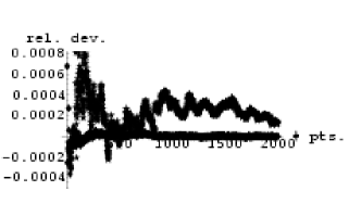
Figure 6: Joint plot of relative deviations of estimates of $V^{s+n}_{SD}$ and $V^{s+n}_{\tilde{KM}}$ from their known and conjectured values of $\frac{\pi^{8}}{5040}$ and $\frac{4\pi^{8}}{315}$. The more rugged curve corresponds to $V^{s+n}_{\tilde{KM}}$.

Further plotting of our various results yielded one of particular interest. In Fig. 7 we show the estimates of $V^{n}_{\tilde{avg}}-V^{n}_{SD}$.

Figure 7: Estimates of the difference, $V^{n}_{\tilde{avg}}-V^{n}_{SD}$, as the number of points in the scrambled Faure-Tezuka sequence increases from 1 million to 2,000 million. Note the strong suggestion that the true value is 25 (or close thereto)

Of course, this figure (the scale of which was internally chosen by MATHEMATICA, based on the data, and not exogeneously imposed) strongly suggests that $V^{n}_{\tilde{avg}}-V^{n}_{SD}=25$. Now, we found that if we posit

$$V^{s+n}_{\tilde{avg}}=\frac{25\pi^{8}}{8448}\approx 28.0792,$$ (18)

(with $8448=2^{8}\cdot 3\cdot 11$), it would follow that

$$V^{n}_{\tilde{avg}}-V^{n}_{SD}=\frac{2449\pi^{8}}{887040}-\frac{26}{9}\sigma_{Ag}\approx 24.99996094,$$ (19)

(with $887040=2^{8}\cdot 3^{2}\cdot 5\cdot 7\cdot 11$), being strikingly close to the indicated value of 25.

In Fig. 8 we plot the deviations of the estimates of $V^{s+n}_{\tilde{avg}}$ from its conjectured value (18).

Figure 8: Deviations of the estimated values of $V^{s+n}_{\tilde{avg}}$ from the conjectured value of $\frac{25\pi^{8}}{8448}$, as the number of points in the scrambled Faure-Tezuka sequence increases from 1 million to 2,000 million

IV Auxiliary analysis

In an independent set of computations (Table 2), employing 415 million points of a scrambled Halton sequence (as opposed to the scrambled Faure-Tezuka sequence used in sec. III), we sought to obtain estimates of the probability of separability of two arbitrarily coupled qubits based on three monotone metrics of interest. The specific method employed was that of scrambled Halton sequences Ökten (1999). (While there are different scrambled Faure-Tezuka sequences depending upon the particular random generating matrices used, the scrambled Halton sequence is unique in nature.)

These correspond to the operator monotone functions,

$$f_{GKS}(t)=t^{t/(t-1)}/e;\quad f_{WY}(t)=\frac{1}{4}(\sqrt{t}+1)^{2};\quad f_{KM}(t)=\frac{t-1}{\log{t}}.$$ (20)

The subscript GKS denotes the Grosse-Krattenthaler-Slater (“quasi-Bures”) metric (which yields the common asymptotic minimax and maximin redundancies for universal quantum coding (Krattenthaler and Slater, 2000, sec. IV.B) Slater (2001)), the subscript WY, the Wigner-Yanase information metric (Gibilisco and Isola, 2003, sec. 4) Wigner and Yanase (1963); Luo (2003), and the subscript KM, the Kubo-Mori metric already studied in secs. II and III. (We had, in fact, intended to study the “Noninformative” monotone metric Slater (1998) here instead of the KM metric, but there was a programming oversight that was only uncovered at the end of the computations.)

Table 2: Estimates based on (four times) the Grosse-Krattenthaler-Slater, Wigner-Yanase and Kubo-Mori monotone metrics, using a scrambled Halton sequence consisting of 415 million points.

metric	$V^{s+n}_{\tilde{metric}}$	$V^{s}_{\tilde{metric}}$	$P^{s}_{metric}=V^{s}/V^{s+n}$
GKS	5.4237	0.330827	.0609965
WY	14.5129	0.730567	.0503391
KM	120.504	4.1791	.0346801

It appears conjecturable that, in terms of the separable states, $V^{s}_{\tilde{GKS}}=\frac{4\sigma_{Ag}}{5}\approx 0.331371$. (The evidence is somewhat of a weaker nature that $V^{s}_{\tilde{WY}}=\frac{7\sigma_{Ag}}{4}\approx 0.724874$.) Also, in terms of the combined separable and nonseparable states, it seems possible that $V^{s+n}_{\tilde{GKS}}=\frac{\pi^{8}}{1750}\approx 5.42202$, with $1750=2\cdot 5^{3}\cdot 7$. If so, we would have $P^{s}_{GKS}=\frac{1400\sigma_{Ag}}{\pi^{8}}\approx 0.0611158$.

We had hoped to further extend the scrambled Halton sequence used here, but doing so has so far proved problematical, in terms of available computer resources.

V Maximal Monotone Metric

As to the maximal monotone metric, numerical, together with some analytical evidence, strongly indicate that $V_{max}^{s+n}$ is infinite (unbounded) (as well as $V^{s}_{max}$). The supporting analytical evidence consists in the fact that for the three-dimensional convex set of $2\times 2$ density matrices, parameterized by spherical coordinates [$r,\theta,\phi$] in the “Bloch ball”, the volume element of the maximal monotone metric is $r^{2}\sin{\theta}(1-r^{2})^{-{3/2}}$, the integral of which diverges over the ball. Contrastingly, the volume element of the minimal monotone metric is $r^{2}\sin{\theta}(1-r^{2})^{-{1/2}}$, the integral over the ball of which is finite, namely $\pi^{2}$. For $s\geq 1$ the integral of $r^{2}\sin{\theta}(1-r^{2})^{-s}$ diverges, so the divergence associated with the monotone metric itself is not simply marginal or “borderline” in character.

To gain further evidence in these regards, one can engage in numerical estimation for the one-parameter family of interpolating metrics given by the operator monotone functions

$$f_{a}(t)=(1-a)f_{max}(t)+af_{Bures}(t),$$ (21)

for which the Morozova-Chentsov functions are of the form

$$c_{a}(\rho_{\mu},\rho_{\nu})=\frac{2(\rho_{\mu}+\rho_{\nu})}{a(\rho_{\mu}-\rho_{\nu})^{2}+4\rho_{\mu}\rho_{\nu}}.$$ (22)

Then, one could plot the results as a function of the parameter $a$ and study the limit $a\rightarrow 0$. (Of course, for $a=\frac{1}{2}$, one would recover the “average” monotone metric, studied in sec. III.)

A preliminary investigation along these lines is reported in Table 3.

Table 3: Estimates based on the first ninety-six million points of a scrambled Faure-Tezuka sequence of (four times) a number of metrics obtained by interpolating between the maximal ($a=0$) and minimal ($a=1$) monotone metrics

a	1	$10^{-1}$	$10^{-2}$	$10^{-3}$	$10^{-4}$	$10^{-5}$	0
$V^{s+n}_{a}$	1.88258	7951.27	$9.3254\cdot 10^{6}$	$6.0345\cdot 10^{9}$	$3.049\cdot 10^{12}$	$1.2825\cdot 10^{15}$	$8.0858\cdot 10^{39}$
$V^{s}_{a}$	0.13786	148.569	63659.	$2.0972\cdot 10^{7}$	$6.502\cdot 10^{9}$	$2.2084\cdot 10^{12}$	$5.229\cdot 10^{36}$
$P^{s}_{a}$	0.073229	0.01868	0.006827	0.003475	0.0021325	0.0017219	0.00064669

Based on the first ninety-six million points of a scrambled Faure-Tezuka sequence, we obtain estimates of $V^{s+n}_{a}$, $V^{s}_{a}$ and $P^{s}_{a}=\frac{V^{s}_{a}}{V^{s+n}_{a}}$ for (four times) the metrics interpolating between the maximal ($a=0$) and minimal ($a=1$) monotone metrics for several values of $a$, increasingly close to $a=0$. So, $P^{s}_{max}$ would seem quite close to being 0. (However, some clearly numerically anomalous behavior occurred in passing from ninety-six million points to ninety-seven million points. The estimates of $V^{s+n}_{max},V^{s}_{max}$ and $P^{s}_{max}$ jumped to $8.27999\cdot 10^{40},7.48026\cdot 10^{40}$ and $0.903414$, respectively.)

It would be interesting to formally test the hypothesis that $P^{s}_{max}=0$. (More specifically, we might ask the question if the limit of $P^{s}_{a}$ as $a\rightarrow 0$ is 0.) If it can, in fact, be established that $P^{s}_{max}$ is zero, this might serve as something in the nature of a “counterexample” to the proposition (a matter of considerable interest in the theoretical analysis of quantum computation) that for bipartite quantum systems of finite dimension, there is a separable neighborhood of the fully mixed state of finite volume Braunstein et al. (1999); Clifton and Halvorson (2000); Gurvits and Barnum (2003); Szarek . (These conclusions were obtained with the use of either the trace or Hilbert-Schmidt metric — the first of which is monotone, but not Riemannian, while the second is Riemannian, but not monotone Sommers and Życzkowski (2003).)

We have conducted a test along these lines. Using a simple Monte-Carlo (rather than quasi-Monte Carlo) scheme, we generated ten sets of ten million points randomly distributed over the 15-dimensional hypercube. For each of the ten sets, we obtained estimates of $V^{s+n}_{max}$, $V^{s}_{max}$ and hence $P^{s}_{max}$. Based on the one hundred million points the (mean) estimate of $P^{s}_{max}$ was $\mu=1.77038\cdot 10^{-7}$ and the standard deviation across the ten samples, $\eta=3.692\cdot 10^{-7}$. So, the value 0 lies less than one-half (that is, 0.479510) standard deviations from $\mu$. For a student $t$-distribution with $9=10-1$ degrees of freedom, forty percent of the probability lies outside 0.261 standard deviations from the mean and twenty-five percent outside 0.703 standard deviations. So there is little evidence here for rejecting a hypothesis that $P^{s}_{max}$ equals 0. For an independent analysis based on ten sets of four million points, the estimates were roughly comparable, i. e., $\mu=2.4196\cdot 10^{-7},\eta=5.09683\cdot 10^{-7}$. Also, for ten sets of five million points, but setting the interpolation parameter $a$ not to 0 but to .05, there were obtained $\mu=.00438593$ and $\eta=.000229437$, with $\frac{\mu}{\eta}=19.1611$. So, here one can decisively reject a hypothesis that the probability of separability for $a=.05$ is 0.

VI Further Monte-Carlo Analyses

We also undertook a series of Monte-Carlo analyses, incorporating together the GKS, Bures, average, Kubo-Mori, Wigner-Yanase, maximal and Noninformative (NI) Slater (1998) monotone metrics. (The operator monotone function $f(t)$ associated with the NI metric is $\frac{2(t-1)^{2}}{(1+t)\log^{2}{(t)}}$.) We subdivide the unit hypercube into $3^{15}=14,348,907$ subhypercubes, pick a random point in each one of these, and then repeat the procedure… We are now able to report in Table 4 the results of fifteen iterations of this process. The central limit theorem tells us that for a large enough sample size, the distribution of the sample mean will approach a normal/Gaussian distribution. This is true for a sample of independent random variables from any population distribution, so long as the population has a finite standard deviation. The population standard deviation is equal to the standard deviation of the mean times the square root of the sample size $N$, which in our case is $15\cdot 3^{15}$. If one were to use two standard deviations as a rejection criterion, then the only one of our conjectures that would be rejected would be that for $V^{s}_{\tilde{GKS}}$. (However, the standard deviations in the separable cases would be approximately four times as large if we only used the number of points corresponding to separable states, rather than to all states, as we have done here. This would lead, then, to none of our conjectures being rejected.)

Table 4: Monte-Carlo analysis based on $15\cdot 3^{15}=215,233,605$ density matrices. The second set of columns correspond to $V^{s}_{\tilde{metric}}$ and the third, to $V^{s+n}_{\tilde{metric}}$. Estimates (est.) of the volumes, standard deviations (s.d.) of these estimates and the number of standard deviations they are away from their conjectured (cj.) or known values, as given in Table 6, are presented

metric	est.	s. d.	$\frac{cj.-est.}{s.d.}$	est.	s. d.	$\frac{cj.-est.}{s.d.}$
Bures	0.13800	0.00021	0.3354	1.88295	0.00102	-0.2985
GKS	0.32990	0.00057	2.5696	5.4232	0.00315	-0.3867
WY	0.72811	0.00152	—	14.5084	0.00943	—
Avg	1.3363	0.00287	-0.5821	28.0781	0.01769	0.0618
KM	4.1574	0.02242	-0.6792	120.256	0.17489	1.3363
NI	848.05	28.997	—	48668.2	421.712	—

The estimate of $P^{s}_{max}$, obtained in the same Monte-Carlo procedure, was $\frac{4.33981\cdot 10^{42}}{1.93678\cdot 10^{52}}=2.24073\cdot 10^{-10}$.

VII 14-Dimensional Boundaries

VII.1 Initial analyses

In the analyses above, we have been concerned with the volume of the 15-dimensional convex set of $4\times 4$ density matrices, as measured in terms of a number of monotone metrics. We have modified the computer programs involved, so that they would provide estimates of the volume (“hyperarea”) of the boundary of this set.

Our numerical integrations were conducted over a fourteen-dimensional hypercube, now allowing one of the original fifteen variables (specifically, the hyperspherical angle designated $\theta_{3}$ in (Slater, 2002, eq. (2))) to be determined not by the quasi-Monte Carlo procedure, but by the requirement that the determinant of the partial transpose equal zero. This considerably increases the computational effort per point generated.

Our early estimates, in this regard, were: 0.587532 (SD), 6.25466 ($\tilde{avg}$) and 19.8296 ($\tilde{KM}$), all three based on the first 2,600,000 points of a scrambled Faure-Tezuka sequence; 1.47928 ($\tilde{GKS}$), 3.37384 ($\tilde{WY}$) and 19.9277 ($\tilde{KM}$), all three based on the first 1,500,000 points of a scrambled Halton sequence; and 0.588816 (a=1), 837.072 $(a=10^{-1})$, 414676. $(a=10^{-2})$, $1.57088\cdot 10^{8}$ $(a=10^{-3})$, $4.87246\cdot 10^{10}$ $(a=10^{-4})$, $1.30774\cdot 10^{13}$ $(a=10^{-5})$, $8.57852\cdot 10^{27}$ $(a=0)$ (all seven based on the first 1,100,000 points of a scrambled Faure sequence).

Let us note that in terms of the Bures metric — identically one-fourth of the statistical distinguishability (SD) metric — the pure state [rank 1] boundary of the $4\times 4$ density matrices, both separable and nonseparable, is known to have volume $\frac{\pi^{3}}{6}\approx 5.16771$. (This is equal to the volume of a 6-dimensional ball of radius 1 and to the volume of a 3-dimensional complex projective space (Sommers and Życzkowski, 2003, sec. IV.C).) The 14-dimensional Bloore (1976) submanifold of $4\times 4$ density matrices of rank 3 has Bures volume $\frac{\pi^{7}}{4324320}\approx 6.98444\cdot 10^{-4}$. Multiplying by $2^{14}$, we obtain the SD counterpart to this of

$$B_{SD}^{s+n}=\frac{512\pi^{7}}{135135}\approx 11.4433.$$ (23)

This is twice (a “double-covering”) the $(n-1)$-content (surface area or hyperarea) of the unit sphere in $n=15$ dimensions.

VII.2 Further analysis

Subsequently, we joined all the monotone metrics of interest into a single joint analysis, using an independent Faure-Tezuka sequence of points in the 14-dimensional hypercube. Up to this point in time, we have generated thirty-five million points (Table 5).

Table 5: Estimates of $14$-dimensional boundary volumes based on (four times) the Bures, Grosse-Krattenthaler-Slater, Wigner-Yanase, Average, Kubo-Mori and Noninformative metrics, using a scrambled Faure-Tezuka sequence composed of thirty-five million points.

metric	$B^{s}$	$B^{s+n}$	$\beta$
Bures	0.456593	11.4443	0.584072
GKS	—	—	1.45204
WY	3203.81	17576.3	6606.58
Avg	6.60067	246.716	6.20592
KM	—	—	19.6215
NI	—	—	4333.36

For each of these points, we sought values of the fifteenth coordinate — $\theta_{3}$ — for which the partial transpose of the corresponding $4\times 4$ density matrix had zero determinant. For 24,038,658 of the points at least one feasible value of $\theta_{3}$ was found. The even-numbered solutions strongly dominated the odd-numbered solutions. (This may pertain to the fact that in this series of analyses, we had used — adjusting accordingly — the range $[0,\pi]$, rather than $[0,\frac{\pi}{2}]$, as in our other analyses, for $\theta_{1},\theta_{2}$ and $\theta_{3}$.) There were 74 points with one solution, 30 with three, and 11 with five, while there were 2,553,168 with two, 21,312,933 with four, 172,429 with six and 3 with eight.

In Fig. 9, we show the cumulative approximations (in steps of one hundred thousand points) to the known value (23) of $B_{SD}^{s+n}$.

Figure 9: Deviations of the estimated value of $B^{s+n}_{SD}$ from the known value of $\frac{512\pi^{7}}{135135}\approx 11.4433$, as the number of points in a certain scrambled Faure-Tezuka sequence increases from one hundred thousand to thirty-five million

We conjecture (Fig. 10) that the component of $B^{s+n}_{SD}$ consisting of separable states Shi and Du , that is $B^{s}_{SD}$, has the value $\frac{43\sigma_{Ag}}{39}\approx 0.456697$.

Figure 10: Deviations of the cumulative estimates of $B^{s}_{SD}$ from the conjectured value of $\frac{43\sigma_{Ag}}{39}\approx 0.456697$. The number of points are recorded in steps of 100,000.

The concomitant estimate of the SD/Bures probability of separability of such rank-three states would then be

$$\Pi^{s}_{SD/Bures}=\frac{B^{s}_{SD}}{B^{s+n}_{SD}}=\frac{297297\sigma_{Ag}}{1024\pi^{7}}\approx 0.0398167.$$ (24)

This is considerably less than the general probability of separability [of, generically, rank-four states], conjectured in formula (16) to be 0.0733389. The ratio of these two probabilities is $\frac{14157\pi}{81920}\approx 0.542194$.

In Fig. 11, we show the cumulative approximations to a conjectured value of $\beta_{SD}=\frac{55\sigma_{Ag}}{39}\approx 0.584147$ for the 14-dimensional SD boundary of separable two-qubit states composed of generically rank-four states. (The test for membership in this class is that the determinant of the partial transpose of the corresponding $4\times 4$ density matrix be zero.)

Figure 11: Deviations from the conjectured value of $\beta_{SD}=\frac{55\sigma_{Ag}}{39}\approx 0.584147$ of the cumulative estimates of the SD volume of that part of the 14-dimensional boundary of the separable states consisting of nondegenerate states. The number of points are recorded in steps of 100,000.

Thus, we have an implied conjecture that the 14-dimensional boundary of separable $4\times 4$ density matrices has total SD-volume of $\beta_{SD}+B^{s}_{SD}=\frac{98\sigma_{Ag}}{39}\approx 1.04084$. The fit of our cumulative estimates to this conjecture is shown in Fig. 12.

Figure 12: Deviations from the conjectured value of $B^{s}_{SD}+\beta_{SD}=\frac{98\sigma_{Ag}}{39}\approx 1.04084$ of the SD-volume of the total boundary of separable states — composed of nondegenerate (rank-four) and degenerate (rank-three) $4\times 4$ density matrices. The number of points of the Faure-Tezuka sequence are recorded in steps of 100,000.

Numerical evidence (Fig. 13) also possibly suggests that $B^{s}_{\tilde{avg}}=\frac{255\sigma_{Ag}}{16}\approx 6.60153$; that (Fig. 14) $B^{s}_{\tilde{WY}}=7735\sigma_{Ag}\approx 3203.94$; that (Fig. 15) $B^{s+n}_{\tilde{WY}}=2^{9}\cdot 3B^{s+n}_{SD}\approx 17576.9$; that (Fig. 16) $\beta_{\tilde{KM}}=\frac{616\sigma_{Ag}}{13}\approx 19.6274$; and that (Fig. 17), $\beta_{\tilde{GKS}}=\frac{270\sigma_{ag}}{77}\approx 1.45244$.

Figure 13: Deviations from the conjectured value of $\frac{255\sigma_{Ag}}{16}\approx 6.60153$ of the cumulative estimates of $B^{s}_{\tilde{avg}}$.

Figure 14: Deviations from the conjectured value of $7735\sigma_{Ag}\approx 3203.94$ of the cumulative estimates of $B^{s}_{\tilde{WY}}$

Figure 15: Deviations from the conjectured value of $B^{s+n}_{\tilde{WY}}$ of $\frac{262144\pi^{7}}{45045}=2^{9}\cdot 3B^{s+n}_{SD}\approx 17576.9$.

Figure 16: Deviations from the conjectured value of $\beta_{\tilde{KM}}=\frac{616\sigma_{Ag}}{13}\approx 19.6274$

Figure 17: Deviations from the conjectured value of $\beta_{\tilde{GKS}}=\frac{270\sigma_{Ag}}{77}\approx 1.45244$

So, surprisingly, the probability of separability of a rank-three state appears to be much higher, that is, $\frac{348423075\sigma_{Ag}}{262144\pi^{7}}=\frac{3^{2}\cdot 5^{2}\cdot 7^{2}\cdot 11\cdot 13^{2}\cdot 17\sigma_{Ag}}{2^{18}\pi^{7}}\approx 0.182281$ using the Wigner-Yanase metric (but not the average metric, for which we have a sample estimate of 0.0267541 and a conjecture of $\frac{10729125\sigma_{Ag}}{54992\pi^{7}}\approx 0.0267572$) than with the Bures or SD metric, in strong contrast to the rank-four case examined earlier (secs. III and IV).

As is apparent, there are no estimates reported in Table 5 for $B^{s}$ and $B^{s+n}$ for the GKS, KM and NI metrics. In retrospect, we could have included the GKS metric (taking the limit of the corresponding volume element as one of the eigenvalues of the associated $4\times 4$ density matrix approaches zero), but the volume elements for the other two were found to diverge on the rank-three states, so they could not have been included.

VII.3 Levy-Gromov Isoperimetric Inequality

The scalar curvature of the Bures metric for the $4\times 4$ density matrices is bounded below by 570 (Dittmann, 1999b, Cor. 3). However, application of the Levy-Gromov Isoperimetric Inequality (Gromov, 1999, App. C) requires a lower bound of $N$ on $Ricci(Y,Y)$, where $Ricci$ is the Ricci tensor and $Y$ runs over all unit tangent vectors, for closed $(N+1)$-dimensional manifolds, We did not immediately know if this condition is satisfied or not (given that one can not apparently “control” the Ricci curvature in terms of the [bounded] scalar curvature), but we have found that the inequality is violated, and that the condition is not satisfied in the case before us.

To reach this conclusion, we first took the parameter $\alpha$ (strictly following the notation in Gromov (1999)) to be $P_{SD/Bures}=\frac{V^{s}_{SD}}{V^{s+n}_{SD}}\approx 0.0736881$, according to our conjecture (6) above. Then, the function $s(\alpha)$ is the 14-dimensional volume of the boundary sphere $\partial B_{\alpha}$, where the volume of the ball $B_{\alpha}$ itself is equal to $\alpha$ $vol(S^{15})$, and $S^{15}$ is the standard 15-dimensional sphere. Further, the function $Is_{15}(\alpha)$ is the ratio of $s(\alpha)\approx 0.499459$ to $vol(S^{15})=\frac{256\pi^{7}}{2027025}\approx 0.381443$. The Levy-Gromov Inequality then asserts that $Is_{15}(\alpha)$, which here equals 1.30939, must be less than a certain ratio, which in our case would — according to our conjectures and known values — be

$$\frac{B^{s}_{Bures}+\beta_{Bures}}{V^{s+n}_{Bures}}=\frac{2^{-14}(B^{s}_{SD}+\beta_{SD})}{2^{-15}V^{s+n}_{SD}}\approx 1.10573.$$ (25)

So, the indicated inequality is violated.

At this point, we applied formula (7a) of Dittmann (1999b), giving the Ricci tensor based on the Bures metric for diagonal density matrices,

$$Ricci(Y,Z)=3\Sigma_{\mu,\nu,\eta}\frac{Y_{\nu\mu}\rho_{\eta}Z_{\mu\nu}}{(\rho_{\mu}+\rho_{\nu})(\rho_{\mu}+\rho_{\eta})(\rho_{\nu}+\rho_{\eta})}-\frac{3}{2}\Sigma_{\mu,\nu}\frac{Y_{\mu\mu}Z_{\nu\nu}}{(\rho_{\mu}+\rho_{\nu})^{2}},$$ (26)

where $Y$ and $Z$ are tangent vectors (traceless Hermitian matrices). We, in fact found, using numerical simulations, violations of the lower bound of $N$ for $(N-1)$-dimensional manifolds on the Ricci tensor required by the Levy-Gromov Inequality, with $N=14$ in our case. The lowest value we were able to achieve in a series of simulations was 3.45666, so no negative values were recorded. (The upper value appeared to be unbounded. We also applied the formula (26) to the 8-dimensional convex set of $3\times 3$ density matrices and found, through Monte Carlo simulations, a value of the Ricci curvature as low as 3.00332, so it appears conjecturable that 3 is the actual lower bound.) Thus, our evidence here indicates that the inequality is not satisfied, apparently since all the conditions for its application have not been met. (Using the ansatz elaborated upon earler in sec. I.3, we also found numerically for the Average and WY monotone metrics that the lower bound of $N=14$ on the Ricci tensor was violated.)

VII.3.1 Area/Volume ratios

Let us also note here (cf. (Życzkowski and Sommers, 2003, sec. 6)), in terms of the known values Sommers and Życzkowski (2003) and our conjectures, that for the separable plus nonseparable states, the ratio of the SD 14-dimensional hyperarea to the SD 15-dimensional volume, is

$$\frac{B^{s+n}_{SD}}{V^{s+n}_{SD}}=\frac{8192}{429\pi}\approx 6.07831$$ (27)

while for only the separable states, it is

$$\frac{B^{s}_{SD}+\beta_{SD}}{V^{s}_{SD}}=\frac{98}{13}\approx 7.53846.$$ (28)

VIII Concluding Remarks

Needless to say, to the extent any of the conjectures above are, in fact, valid ones, their remains the apparently formidable task of finding formal/rigorous proofs.

A direct/naive “brute force” strategy of symbolically integrating the volume elements of the various monotone metrics over the 15-dimensional convex sets of separable and all two-qubit states — while successful for lower-dimensional scenarios Slater (2000) — appears to be quite impractical computationally-speaking. It seems that one would have to deal with multiple ranges of integration given by fourth-degree polynomials. One might speculate that the integration of the (product) measures for the volume elements of monotone metrics over the twelve parameterizing Euler angles would yield a result simply proportional to $\sigma_{Ag}$, common to all monotone metrics, and that additional distinguishing factors would appear from integrating over the final three variables ($\theta_{1},\theta_{2},\theta_{3}$ in the notation of Slater (2002)) parameterizing the eigenvalues of the $4\times 4$ density matrices.

Perhaps, in this regard, the work of Sommers and Życzkowski Sommers and Życzkowski (2003) — which they view “as a contribution to the theory of random matrices” — in constructing a general formula for $V^{s+n}_{Bures}$ for $N$-level systems, is extendible to (monotone) metrics other than the Bures. The volume $V^{s+n}_{SD}$ is known, and we have indicated our conjectures that $V^{s+n}_{\tilde{KM}}=64V^{s+n}_{SD},V^{s+n}_{\tilde{avg}}=\frac{25\pi^{8}}{8448},V^{s+n}_{\tilde{GKS}}=\frac{\pi^{8}}{1750}$ and $V^{s+n}_{\tilde{max}}=\infty$, but we have no similar conjecture, at the present, for $V^{s+n}_{\tilde{WY}}$. (The Wigner-Yanase metric corresponds to a space of constant curvature Gibilisco and Isola (2003).) But there appears to be no “hint” in the literature as to how one might formally derive simply the separable — as opposed to separable plus nonseparable — volumes for any of the monotone metrics.

In this study, we have conjectured that the volumes of separable two-qubit states is, as measured in terms of several monotone metrics of interest, simple multiples of the silver mean ($\sigma_{ag}$). It is interesting to point out, it seems, that in certain (“phyllotactic”) models of the arrangements of (rose) petals, the positions of the petals (in fractions of a full turn) are given by the fractional parts of simple multiples of the golden ratio (Livio, 2002, p. 113) (Conway and Guy, 1996, pp. 122-123) (cf. (Freedman, 2003, p. 137)). (Of course, it remains possible that we have been somewhat “overeager” here to find multiple roles for $\sigma_{Ag}$. In this regard, a sceptically-inclined reader might point out that $2000\sigma_{br}\approx 6605.55$ is quite close to our sample estimate of 6606.58 (Table 5) for $\beta_{\tilde{WY}}$ and $2\sigma_{br}\approx 6.60555$ approximates our sample estimate of 6.60067 for $B^{s}_{\tilde{avg}}$. Here, $\sigma_{br}=\frac{3+\sqrt{13}}{2}$ is the “bronze mean” Gumbs (1989).)

In this and other papers Slater (2002); Życzkowski et al. (1998); Życzkowski (1999); Slater (1999a, 2000); Życzkowski and Sommers (2003), attention has been focused on the matter of determining the volumes of quantum states in terms of various monotone metrics. An even more considerable body of work concerned with differential geometric properties of the monotone metrics is devoted to issues of the scalar curvature of monotone metrics Gibilisco and Isola (2003); Andai (2003); Dittmann (1999c). For instance, it has been found that the scalar curvature of the $N\times N$ density matrices $D_{N}$ is, in terms of the Wigner-Yanase metric, $\frac{1}{4}(N^{2}-1)(N^{2}-2)$ Gibilisco and Isola (2003), while for the Bures metric, it is 24 for $N=2$ and for general $N$, no less than $\frac{1}{2}{(5N^{2}-4)(N^{2}-1)}$, which value is assumed for the fully mixed state $\frac{1}{N}\bf{I}$ Dittmann (1999c). (For the infinite-dimensional case of thermal squeezed states, Twamley (Twamley, 1996, eq. (30)) has found the scalar curvature to be given by $-\frac{8(\cosh^{2}{\beta/4}+12\sinh^{4}{\beta/4})}{\cosh^{2}{\beta/2}}$, where the “non-unitary” parameter $\beta$ corresponds to the inverse temperature.) It would certainly be of interest to find linkages between these two interesting areas of investigation. We note that the scalar curvature determines the asymptotic behavior of the volume of a Riemannian manifold Gibilisco and Isola (2003) (Sakai, 1996, p. 55, Cor. 5.5 and ex. 3). Andai (Andai, , eq. (1)) has recently presented a formula for the relation between the volume of a geodesic ball centered at the fully mixed state and the scalar curvature there (see also (Petz, 2002, eq. (29))).

Our earlier conjecture (3) — in its unadjusted form — as to the exact value of $V^{s}_{SD}$ had suggested a similar-type conjecture for qubit-qutrit pairs Slater (2003). Now that we have found compelling numerical evidence to reject (3) (and replace it by (15)), we obviously must be dubious as to the presumed validity of its qubit-qutrit analogue, but presently lack any notion as to how to replace it. Additionally, our numerical experience so far indicates that it would be extraordinarily difficult to “pinpoint” (accurately estimate) the value of the volume of separable qubit-qutrit pairs, since one would then be proceeding in a (more computationally demanding) much higher-dimensional (35-d v. 15-d) space, plus the size of the separable domain one would be estimating would be much smaller relatively speaking (that is, relatively fewer sampled $6\times 6$ density matrices would be separable vis-á-vis the $4\times 4$ case).

We summarize in Table 6 our present state of presumed knowledge in regard to the various monotone metrics studied here. Of course, one would aspire to find the functionals that map an operator monotone function $f_{metric}(t)$ into $V^{s}_{metric},V^{s+n}_{metric},B^{s}_{metric},B^{s+n}_{metric}$ and $\beta_{metric}$.

Table 6: Conjectured values (except for $V^{s+n}_{\tilde{Bures}}$ and $B^{s+n}_{\tilde{Bures}}$, which are known) of $V^{s}_{\tilde{metric}}$, $V^{s+n}_{\tilde{metric}}$, $B^{s+n}_{\tilde{metric}}$, $B^{s}_{\tilde{metric}}$ and $\beta_{\tilde{metric}}$ for (four times) various monotone metrics, listed in order of increasing volume size, together with the corresponding operator monotone functions and Morozova-Chentsov functions. (For the various denominators, we have the interesting prime decompositions: $5040=2^{4}\cdot 3^{2}\cdot 5\cdot 7$; $1750=2\cdot 5^{3}\cdot 7$; $8448=2^{8}\cdot 3\cdot 11$; $315=3^{2}\cdot 5\cdot 7$; $135135=3^{3}\cdot 5\cdot 7\cdot 11\cdot 13$; $42075=3^{2}\cdot 5^{2}\cdot 11\cdot 17$ and $45045=3^{2}\cdot 5\cdot 7\cdot 11\cdot 13$. As pertains to numerators: $512=2^{9}$; $7735=5\cdot 7\cdot 13\cdot 17$; $262144=2^{18}$; $15950=2\cdot 5^{2}\cdot 11\cdot 29$; $255=3\cdot 5\cdot 17$; $495=3^{3}\cdot 5\cdot 11$; $270=2\cdot 3^{3}\cdot 5$; and $616=2^{3}\cdot 7\cdot 11$.)

metric	$f(t)$	$c(\rho_{\mu},\rho_{\nu})$	$V^{s}$	$V^{s+n}$	$B^{s}$	$B^{s+n}$	$\beta$	$B^{s}+\beta$
Bures	$\frac{1+t}{2}$	$\frac{2}{\rho_{\mu}+\rho_{\nu}}$	$\frac{\sigma_{Ag}}{3}$	$\frac{\pi^{8}}{5040}$	$\frac{43\sigma_{Ag}}{39}$	$\frac{512\pi^{7}}{135135}$	$\frac{55\sigma_{Ag}}{39}$	$\frac{98\sigma_{Ag}}{39}$
GKS	$\frac{t^{t/(t-1)}}{e}$	$\frac{e(\frac{\rho_{\mu}}{\rho_{\nu}})^{\frac{\rho_{\mu}}{\rho_{\nu}-\rho_{\mu}}}}{\rho_{\nu}}$	$\frac{4\sigma_{Ag}}{5}$	$\frac{\pi^{8}}{1750}$	?	?	$\frac{270\sigma_{Ag}}{77}$	?
WY	$\frac{(\sqrt{t}+1)^{2}}{4}$	$\frac{4}{(\sqrt{\rho_{\mu}}+\sqrt{\rho_{\nu}})^{2}}$	$\frac{7\sigma_{Ag}}{4}$	?	$7735\sigma_{Ag}$	$\frac{262144\pi^{7}}{45045}$	$15950\sigma_{Ag}$	$23685\sigma_{Ag}$
Avg	$\frac{1+6t+t^{2}}{4+4t}$	$\frac{4(\rho_{\mu}+\rho_{\nu})}{\rho_{\mu}^{2}+6\rho_{\mu}\rho_{\nu}+\rho_{\nu}^{2}}$	$\frac{29\sigma_{Ag}}{9}$	$\frac{25\pi^{8}}{8448}$	$\frac{255\sigma_{Ag}}{16}$	$\frac{3437\pi^{7}}{42075}$	$15\sigma_{Ag}$	$\frac{495\sigma_{Ag}}{16}$
KM	$\frac{t-1}{\log{t}}$	$\frac{\log{\frac{\rho_{\mu}}{\rho_{\nu}}}}{\rho_{\mu}-\rho_{\nu}}$	$10\sigma_{Ag}$	$\frac{4\pi^{8}}{315}$	$\infty$	$\infty$	$\frac{616\sigma_{Ag}}{13}$	$\infty$
NI	$\frac{2(t-1)^{2}}{(1+t)(\log{t})^{2}}$	$\frac{(\rho_{\mu}+\rho_{\nu}){\log^{2}{\frac{\rho_{\mu}}{\rho_{\nu}}}}}{2(\rho_{\mu}-\rho_{\nu})^{2}}$	?	?	$\infty$	$\infty$	?	$\infty$
maximal	$\frac{2t}{1+t}$	$\frac{\rho_{\mu}+\rho_{\nu}}{2\rho_{\mu}\rho_{\nu}}$	$\infty$	$\infty$	$\infty$	$\infty$	$\infty$	$\infty$