Gaussian quantum operator representation for bosons

Abstract

We introduce a Gaussian quantum operator representation, using the most general possible multi-mode Gaussian operator basis. The representation unifies and substantially extends existing phase-space representations of density matrices for Bose systems, and also includes generalized squeezed-state and thermal bases. It enables first-principles dynamical or equilibrium calculations in quantum many-body systems, with quantum uncertainties appearing as dynamical objects. Any quadratic Liouville equation for the density operator results in a purely deterministic time evolution. Any cubic or quartic master equation can be treated using stochastic methods.

I Introduction

In this paper we develop a general multi-mode Gaussian representation for a density matrix of bosons. As well as classical phase-space variables like $(\mathbf{x},\mathbf{p})$, the representation utilizes a dynamical space of quantum uncertainties or co-variances. The extended phase space accommodates more efficiently the content of a quantum state, and allows the physics of many kinds of problems to be incorporated into the basis itself. The Gaussian expansion technique unifies and greatly extends all the previous Gaussian-like phase-space representations used for bosons, including the Wigner, $Q$, $P$, positive-$P,$ and squeezed-state expansions. The operator basis also includes non-Hermitian Gaussian operators, which are not density matrices themselves, but can form part of a probabilistic expansion of a physical density matrix. Unlike previous approaches, any initial state is found to evolve with a deterministic time-evolution under any quadratic Hamiltonian or master equation.

The complexity of many-body quantum physics is manifest in the enormity of the Hilbert space of systems with even modest numbers of particles. This complexity makes it prohibitively difficult to simulate quantum dynamics with exact precision: no digital computer is large enough to store the dynamically evolving state. However, if a finite precision is permitted, then quantum dynamical calculations are possible, through what are known as phase-space methods. These methods represent the evolving quantum state as probability distributions on some suitable phase space, which can be sampled via stochastic techniques. The mapping to phase space can be made to be exact. Thus the precision of the final result is limited only by sampling error, which can usually be reliably estimated and which can be reduced by an increased number of stochastic paths.

Arbitrary quantum mechanical evolution cannot be represented (even probabilistically) on a phase space as is usually defined. Thus the extended phase spaces employed here are a generalization of conventional phase spaces in several ways. First, it is a quantum phase space, in which points can correspond to states with intrinsic uncertainty. Heisenberg’s uncertainty relations can thus be satisfied in this way, or more generally by considering genuine probability distributions over phase space, to be sampled stochastically. Second, the phase space is of double dimension, where classically real variables, such as $\mathbf{x}$ and $\mathbf{p}$, now range over the complex plane. This allows arbitrary quantum evolution to be sampled stochastically. Third, stochastic gauge variables are included. These arbitrary quantities do not affect the physical results, but they can be used to overcome problems in the stochastic sampling. Fourth, the phase space includes the set of second-order moments, or covariances. A phase space that is enlarged in this way is able to accommodate more information about a general quantum state in a single point. In particular, any state (pure or mixed) with Gaussian statistics can be represented as a single point in this phase space.

The Gaussian representation provides a link between phase-space methods and approximate methods used in many-body theory, which frequently treat normal and anomalous correlations or Green’s functions as dynamical objectsBaymKad . As well as being applicable to quantum optics and quantum information, a strong motivation for this representation is the striking experimental observation of BEC in ultra-cold atomic systemsobsex1 . Already the term ‘atom laser’ is widely used, and experimental observation of quantum statistics in these systems is underway. Yet there is a problem in using previous quantum optics formalisms to calculate coherence properties in atom optics: interactions are generally much stronger with atoms than they are with photons, relative to the damping rate. The consequence of this is that one must anticipate larger departures from ’semiclassical’, coherent-state behaviour in atomic systems.

The present paper includes these nonclassical and incoherent effects at the level of the basis for the operator representation itself. The purpose of employing a Gaussian basis set is not only to enlarge the parameter set (to hold more information about the quantum state), but also to include in the basis states that are a close match to the actual states that are likely to occur in interesting systems, such as dilute gases. The pay-off for increasing the parameter set is more efficient sampling of the dynamically evolving or equilibrium states of many-body systems.

The idea of coherent states as a quasi-classical basis for quantum mechanics originated with SchrödingerScrod . Subsequently, Wigner Wig-Wigner introduced a distribution for quantum density matrices. This method was a phase-space mapping with classical dimensions and employed a symmetrically ordered operator correspondence principle. Later developments included the antinormally ordered $Q$ distributionHus-Q , a normally ordered expansion called the diagonal $P$ distributionGla-P , methods that interpolate between these classical phase-space distributionsCG-Q ; Agarwal , and diagonal squeezed-state representationsSchCav84 . Each of these expansions either employs an explicit Gaussian density matrix basis or is related to one that does by convolution. They are suitable for phase-space representations of quantum states because of the overcompleteness of the set of coherent states on which they are based.

Arbitrary pure states of bosons with a Gaussian wave-function or Wigner representation are often called the squeezed statesSqueeze . These are a superset of the coherent states, and were investigated by BogoliubovBogol to approximately represent the ground state of an interacting Bose-Einstein condensate - as well as in much recent work in quantum opticsQOSqueeze . Diagonal expansions analogous to the diagonal $P$-representation have been introduced using a basis of squeezed-state projectors, typically with a fixed squeezing parameterSchCav84 . However, these have not generally resulted in useful dynamical applications, as they do not overcome the problems inherent in using a diagonal basis, as we discuss below.

In operator representations, one must utilize a complete basis in the Hilbert space of density operators, rather than in the Hilbert space of pure states. Thermal density matrices, for example, are not pure states, but do have a Gaussian $P$ representation and Wigner function. To include all three types of commonly used Gaussian states - the coherent, squeezed and thermal states - one can define a Gaussian state as a density matrix having a Gaussian positive-$P$ or Wigner representationLindbladgauss . This definition also includes displaced and squeezed thermal states. Gaussian states have been investigated extensively in quantum information and quantum entanglementGaussQI . It has been shown that an initial Gaussian state will remain Gaussian under linear evolutionBartlett .

However, the Gaussian density matrices that correspond to physical states do not by themselves form a complete basis for the time-evolution of all quantum density matrices. This problem, inherent in all diagonal expansions, is related to known issues in constructing quantum–classical correspondencesNeumann , and is caused by the non-positive-definite nature of the local propagator in a classical phase space. It is manifest in the fact that there is generally no equivalent Fokker-Planck equation (with a positive-definite diffusion matrix) that generates the quantum time-evolution, and hence no corresponding stochastic differential equation that can be efficiently simulated numerically. This difficulty occurs in nearly all cases except free fields, and represents a substantial limitation in the use of these diagonal expansion methods for exact simulation of the quantum dynamics of interacting systems.

These problems can be solved by use of nonclassical phase spaces, which correspond to expansions in non-Hermitian bases of operators (rather than just physical density matrices). One established example is the non-diagonal positive-$P$DG-PosP representation. The non-Hermitian basis in this case generates a representation with a positive propagator, which allows the use of stochastic methods to sample the quantum dynamics. By extending the expansion to include a stochastic gauge freedom in these evolution equations, one can select the most compact possible time-evolution equationgauge_paper ; Paris1 ; Plimak . With an appropriate gauge choice, this method is exact for a large class of nonlinear Hamiltonians, since it eliminates boundary terms that can otherwise ariseGGD-Validity . The general Gaussian representation used here also includes these features, and extends them to allow treatment of any Hamiltonian or master equation with up to fourth-order polynomial terms.

Other methods of theoretical physics that have comparable goals are the path-integral techniques of quantum field theorywilson:74 ; Ceperley , and density functional methodsKohn that are widely used to treat atomic and molecular systems. The first of these is exact in principle, but is almost exclusively used in imaginary time calculations of canonical ensembles or ground states due to the notorious phase problem. The second method has similarities with our approach in that it also utilizes a density as we do. However, density functionals are normally combined with approximations like the local density approximation. Gaussian representation methods have the advantage that they can treat both real and imaginary time evolution. In addition, the technique is exact in principle, provided boundary terms vanish on partial integration.

In section II, we define general Gaussian operators for a density operator expansion and introduce a compact notation for these operators, either in terms of mode operators or quantum fields. In section III, we calculate the moments of the general Gaussian representation, relating them to physical quantities as well as to the moments of previous representations. Section IV gives the necessary identities that enable first-principles quantum calculations with these representations.

Equation (LABEL:eq:Matrixidentities) summarizes the relevant operator mappings, and constitutes a key result of the paper.

We give a number of examples in section V of specific pure and mixed states (and their non-Hermitian generalizations) that are included in the basis, and we give simplified versions of important identities for these cases. Section VI describes how the Gaussian representation can be used to deal with evolution in either real or imaginary time. In particular, we show how it can be used to solve exactly any master equation that is quadratic in annihilation and creation operators. Some useful normalization integrals and reordering identities for the Gaussian operators are proved in the Appendices.

In a subsequent paper, we will apply these methods to systems with nonlinear evolution.

II The Gaussian representation

The representations that give exact mappings between operator equations and stochastic equations – an essential step toward representing operator dynamics in large Hilbert spaces – are stochastic gauge expansionsgauge_paper ; Paris1 ; Plimak on a nonclassical phase space. Here, the generic expansion is written down in terms of a complete set of operators that are typically non-Hermitian. This leads to the typical form:

$$\widehat{\rho}(t)=\int P(\overrightarrow{\lambda},t)\widehat{\Lambda}(\overrightarrow{\lambda})d\overrightarrow{\lambda}\,\,,$$ (1)

where $P(\overrightarrow{\lambda},t)$ is a probability distribution, $\widehat{\Lambda}$ is a suitable basis for the class of density matrices being considered, and $d\overrightarrow{\lambda}$ is the integration measure for the corresponding generalized phase-space coordinate $\overrightarrow{\lambda}$. See Fig. 1 for a conceptual illustration of this expansion.

In phase-space methods, it is the distribution $P$ that is sampled stochastically. Therefore if the basis resembles the typical physical states of a system, the sampling error will be minimized, and if the state coincides exactly with an element of the basis, then the distribution will be a delta function, with consequently no sampling error. A Wigner or $Q$-function basis, for example, generates a broad distribution even for minimum uncertainty states. A general Gaussian basis, on the other hand, can generate a delta-function distribution not only for any minimum uncertainty state, but also for the ground states of non-interacting finite-temperature systems.

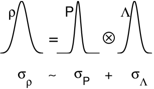
Figure 1: The density-operator expansion in Eq. (1) can be interpreted as a convolution of the probability distribution $P$ with the underlying distribution of the basis. The uncertainty or spread of the physical state, indicated by the variance $\sigma_{\rho}$, is shared between the distribution variance $\sigma_{P}$ and the basis variance $\sigma_{\Lambda}$.

II.1 Gaussian operator basis

In this paper, we define the operator basis $\widehat{\Lambda}$ to be the most general Gaussian operator basis. The motivation for using the most general possible basis set is that when the basis set members nearly match the states of interest, the resulting distributions are more compact and have lower sampling errors in a Monte-Carlo or stochastic calculation. In addition, a larger basis allows more choice of mappings, so that lower-order differential correspondences can be utilized. In some cases, a large basis set can increase computational memory requirements, as more parameters are needed. This disadvantage is outweighed when there is a substantial decrease in sampling error, due to the use of a more physically appropriate basis. By choosing a general Gaussian operator basis, rather than just a basis of Gaussian density matrices, one has the additional advantage of a complete representation for all non-Gaussian density matrices as well.

If $\widehat{\bm{a}}$ is a column vector of $M$ bosonic annihilation operators, and $\widehat{\bm{a}}^{\dagger}$ the corresponding row vector of creation operators, their commutation relations are:

$$\left[\widehat{a}_{k},\widehat{a}_{j}^{\dagger}\right]=\delta_{kj}\,\,.$$ (2)

We define a Gaussian operator as an exponential of an arbitrary quadratic form in annihilation and creation operators (or, equivalently, a quadratic form in position and momentum operators).

The simplest way to achieve this is to introduce extended $2M$-vectors of c-numbers and operators: $\underline{\alpha}=(\,\bm{\alpha},(\bm{\alpha}^{+})^{T})$, and $\underline{\widehat{a}}=(\widehat{\bm{a}},(\widehat{\bm{a}}^{\dagger})^{T})$, with adjoints defined as $\underline{\alpha}^{+}=(\bm{\alpha}^{+},\bm{\alpha}^{T})$ and $\underline{\widehat{a}}^{\dagger}=(\widehat{\bm{a}}^{\dagger},\widehat{\bm{a}}^{T})$, together with a relative operator displacement of

$$\delta\underline{\widehat{a}}=\underline{\widehat{a}}-\underline{\alpha}=\left(\begin{array}[]{c}\widehat{a}_{1}\\ \vdots\\ \widehat{a}_{M}\\ \widehat{a}_{1}^{\dagger}\\ \vdots\\ \widehat{a}_{M}^{\dagger}\end{array}\right)-\left(\begin{array}[]{c}\alpha_{1}\\ \vdots\\ \alpha_{M}\\ \alpha_{1}^{+}\\ \vdots\\ \alpha_{M}^{+}\end{array}\right)\,\,.$$ (3)

These extended vectors are indexed where necessary with Greek indices: $\mu=1,...,2M$.

A general Gaussian operator is now an exponential of a general quadratic form in the $2M$-vector mode operator $\delta\underline{\widehat{a}}$. For algebraic reasons, it is useful to employ normal ordering, and to introduce a compact notation using a generalized covariance $\underline{\underline{\sigma}}$:

$\displaystyle\widehat{\Lambda}(\overrightarrow{\lambda})$ $\displaystyle=$ $\displaystyle\frac{\Omega}{\sqrt{\left|\underline{\underline{\sigma}}\right|}}:\exp\left[-\delta\underline{\widehat{a}}^{\dagger}\underline{\underline{\sigma}}^{-1}\delta\underline{\widehat{a}}/2\right]:\,\,.$ (4)

Here the normalization factor involving $\sqrt{\left|\underline{\underline{\sigma}}\right|}$ is introduced to simplify identities that occur later, and plays a very similar role to the exactly analogous normalization factor that occurs in the classical Gaussian distribution of probability theory. The $2M\times 2M$ covariance matrix is conveniently parameterized in terms of $M\times M$ submatrices as:

$$\underline{\underline{\sigma}}=\left[\begin{array}[]{cc}\mathbf{I}+\mathbf{n}&\mathbf{m}\\ \mathbf{m}^{+}&\mathbf{I}+\mathbf{n}^{T}\end{array}\right]\,\,,$$ (5)

where $\mathbf{n}$ is a complex $M\times M$ matrix and $\mathbf{m},\mathbf{m}^{+}$ are two independent symmetric complex $M\times M$ matrices.

With this choice, the covariance has a type of generalized Hermitian symmetry in which $\sigma_{\mu\nu}=\sigma_{\nu+M,\mu+M}$, provided we interpret the matrix indices as cyclic in the sense that $\nu\sim\nu+2M$. This can also be written as $\underline{\underline{\sigma}}=\underline{\underline{\sigma}}^{+},$with the definition that:

$$\left[\begin{array}[]{cc}\mathbf{a}&\mathbf{b}\\ \mathbf{c}&\mathbf{d}\end{array}\right]^{+}\equiv\left[\begin{array}[]{cc}\mathbf{d}&\mathbf{c}\\ \mathbf{b}&\mathbf{a}\end{array}\right]^{T}\,\,.$$ (6)

This definition implies that we intend the ‘⁺’ superscript to define an operation on the covariance matrix which is equivalent to Hermitian conjugation of the underlying operators. If the Gaussian operator is in fact an Hermitian operator, then so is the corresponding covariance matrix. In this case, the ‘⁺’ superscript is identical to ordinary Hermitian conjugation. The generalized Hermitian symmetry of the covariance means that all elements of the number correlation $\mathbf{n}$ appear twice, as do all except the diagonal elements of the squeezing correlations $\mathbf{m},\mathbf{m}^{+}$.

The use of normal ordering allows simple operator identities to be obtained, but can easily be related to more commonly used unordered parameterizations. The Gaussian operators include as special cases the density matrices of many useful and well-known physical states. For example, they include the thermal states of a Bose-Einstein distribution, the coherent states, and the squeezed states. They also include many more states than these, like the off-diagonal coherent state projectors used in the positive-$P$ expansion, which are not density operators themselves, but can be used to expand density operators. The details are given in section V.

II.2 Extended phase space

The representation phase space is thus extended to

$$\overrightarrow{\lambda}=(\Omega,\bm{\alpha},\bm{\alpha}^{+},\mathbf{n},\mathbf{m},\mathbf{m}^{+})\,\,.$$ (7)

The complex amplitude $\Omega$, which appears in the normalisation, acts as a dynamical weight on different stochastic trajectories. It is useful in calculations in which the normalisation of the density matrix is not intrinsically preserved, such as canonical ensemble calculations, and also enables stochastic gauges to be included.

The complex vectors $\bm{\alpha}$ and $\bm{\alpha}^{+}$ give the generalized coherent amplitudes for each mode: $\bm{\alpha}$ defines the amplitudes of annihilation operators $\widehat{\bm{a}}$ , while its ‘conjugate’ $\bm{\alpha}^{+}$ defines the amplitudes of the creation operators $\widehat{\bm{a}}^{\dagger}$. The matrix $\mathbf{n}$ gives the number, or normal, correlations between each pair of modes. The squeezing, or anomalous, correlations between each pair of modes are given by $\mathbf{m}$ and $\mathbf{m}^{+}$: the matrix $\mathbf{m}$ defines the correlations of annihilation operators, while its ‘conjugate’ $\mathbf{m}^{+}$ defines the correlations of the creation operators. These physical interpretations of the phase-space variables are supported by the results of Section III, where we rigorously establish the connection of the phase-space variables to physical quantities.

In general, apart from the complex amplitude $\Omega$, the total number of complex parameters needed to specify the normalized $M$-mode Gaussian operator is:

$$p=M(2+3M)\,\,.$$ (8)

Hence the phase-space variables can be written as $\overrightarrow{\lambda}=(\lambda_{0},\lambda_{1},...,\lambda_{p})$, with the corresponding integration measure as $d\overrightarrow{\lambda}=d^{2(p+1)}\overrightarrow{\lambda}$.

II.3 Gaussian field operators

The above results define a completely general Gaussian operator in terms of arbitrary bosonic annihilation and creation operators, without reference to the field involved. It is sometimes useful to compare this to a field theoretic notation, in which we explicitly use a coordinate-space integral to define the correlations. This provides a means to extend operator representation theory for fieldsCarter-Drummond ; Kennedy ; becpf ; Drummond-Corney to more general basis sets. In a quantization volume $V$, one can expand:

$$\widehat{\Psi}_{j}(\mathbf{x}) = \frac{1}{\sqrt{V}}\sum_{\mathbf{k}}\widehat{a}_{\mathbf{k},j}e^{i\mathbf{k}.\mathbf{x}}$$

$$\widehat{\Psi}_{j}^{\dagger}(\mathbf{x}) = \frac{1}{\sqrt{V}}\sum_{\mathbf{k}}\widehat{a}_{\mathbf{k},j}^{\dagger}e^{-i\mathbf{k}.\mathbf{x}}\,,$$ (9)

where the field commutators are

$$\left[\widehat{\Psi}_{j}(\mathbf{x}),\widehat{\Psi}_{j^{\prime}}^{\dagger}(\mathbf{x}^{\prime})\right]=\delta_{jj^{\prime}}\delta(\mathbf{x}-\mathbf{x}^{\prime})\,\,.$$ (10)

With this notation, the quadratic term in the Gaussian exponent becomes:

$$\delta\underline{\widehat{a}}^{\dagger}\underline{\underline{\sigma}}^{-1}\delta\underline{\widehat{a}}=\int\int\delta\underline{\widehat{\Psi}}^{\dagger}(\mathbf{x})\underline{\underline{\sigma}}^{-1}(\mathbf{x},\mathbf{y})\delta\underline{\widehat{\Psi}}(\mathbf{y})d^{3}\mathbf{x}d^{3}\mathbf{y}\,\,,$$ (11)

where we have introduced the extended vector $\underline{\widehat{\Psi}}(\mathbf{x})=(\widehat{\bm{\Psi}},\left(\widehat{\bm{\Psi}}^{\dagger}\right)^{T})$, and $\delta\underline{\widehat{\Psi}}(\mathbf{x})=\underline{\widehat{\Psi}}(\mathbf{x})-\underline{\Psi}(\mathbf{x})$ which is the operator fluctuation relative to the coherent displacement or classical mean field. If we index the extended vector as $\Psi_{js}$ , where $s=-1(1)$ for the first and second parts respectively, this Fourier transform can be written compactly as:

$$\Psi_{js}(\mathbf{x})=\frac{1}{\sqrt{V}}\sum_{\mathbf{k}}\alpha_{\mathbf{k}js}e^{-is\mathbf{k}.\mathbf{x}}\,\,.$$ (12)

The notation $\underline{\underline{\sigma}}^{-1}(\mathbf{x},\mathbf{y})$ indicates a functional matrix inverse where:

$$\int\underline{\underline{\sigma}}^{-1}(\mathbf{x},\mathbf{y})\underline{\underline{\sigma}}(\mathbf{y},\mathbf{x}^{\prime})d^{3}\mathbf{y}=\underline{\underline{I}}\delta(\mathbf{x}-\mathbf{x}^{\prime})\,\,,$$ (13)

and the relationship to the previous cross-variance matrix is that:

$$\sigma_{js,j^{\prime}s^{\prime}}(\mathbf{x},\mathbf{y})=\frac{1}{V}\sum_{\mathbf{k}}\sum_{\mathbf{k}^{\prime}}\sigma_{\mathbf{k}js,\mathbf{k}^{\prime}j^{\prime}s^{\prime}}e^{-i(s\mathbf{k}.\mathbf{x}-s^{\prime}\mathbf{k}^{\prime}.\mathbf{x}^{\prime})}\,.$$ (14)

In the standard terminology of many-body theory and field theoryBaymKad , these field variances are generalized equal-time Green’s functions, and can be written as:

$$\underline{\underline{\sigma}}(\mathbf{x},\mathbf{x}^{\prime})=\left[\begin{array}[]{cc}\mathbf{I}\delta(\mathbf{x},\mathbf{x}^{\prime})+\mathbf{n}(\mathbf{x},\mathbf{x}^{\prime})&\mathbf{m}(\mathbf{x},\mathbf{x}^{\prime})\\ \mathbf{m}(\mathbf{x},\mathbf{x}^{\prime})^{+}&\mathbf{I}\delta(\mathbf{x},\mathbf{x}^{\prime})+\mathbf{n}^{T}(\mathbf{x}^{\prime},\mathbf{x})\end{array}\right]\,\,.$$ (15)

We shall show in the next section that these indeed correspond to field correlation functions in the case that the field state is able to be represented as a single Gaussian. More generally, one must consider a probability distribution over different coherent fields and Green’s functions or variances, in order to construct the overall density matrix.

III Gaussian expectation values

In order to use the Gaussian operator basis, a number of basic identities are needed. In this section, we derive relations between operator expectation values and moments of the distribution. Such moments also show how the general Gaussian representation incorporates the previously used methods.

III.1 Gaussian trace

The trace of a generalized Gaussian is needed to normalize the density matrix. The trace is most readily calculated by using a well-known coherent-state identityGla-P ,

$${\rm Tr}\left[\widehat{\Lambda}\right]=\int\left\langle\mathbf{z}\right|\widehat{\Lambda}\left|\mathbf{z}\right\rangle\frac{d^{2M}\mathbf{z}}{\pi^{M}}\,.$$ (16)

Here we define $\mathbf{z}=(z_{1},...,z_{M})$. Next, introducing extended vectors $\underline{z}=(\mathbf{z},\mathbf{z}^{\ast})^{T}$, $\underline{z}^{+}=(\mathbf{z}^{*},\mathbf{z})$, $\delta\underline{z}=\underline{z}-\underline{\alpha}$, and using the eigenvalue property of coherent states, $\widehat{\bm{a}}\left|\mathbf{z}\right\rangle=\mathbf{z}\left|\mathbf{z}\right\rangle$, we find that:

$${\rm Tr}\left[\widehat{\Lambda}\right]=\frac{\Omega\int d^{2M}\mathbf{z}\exp\left[-\delta\underline{z}^{+}\underline{\underline{\sigma}}^{-1}\delta\underline{z}/2\right]}{\pi^{M}\sqrt{\left|\underline{\underline{\sigma}}\right|}}\,\,.$$ (17)

The normalizing factor can now be recognized as the determinant expression arising in a classical Gaussian. For example, in the single-mode case, one obtains for the normalizing determinant that:

$$\frac{1}{\sqrt{\left|\underline{\underline{\sigma}}\right|}}=\frac{1}{\sqrt{(1+n)^{2}-mm^{+}}\,}\,.$$ (18)

We can thus calculate the value of the normalization from standard Gaussian integrals, as detailed in Appendix B, provided $\underline{\underline{\sigma}}$ has eigenvalues with a positive real part. The result is:

$${\rm Tr}\left[\widehat{\Lambda}\right]=\Omega\,\,.$$ (19)

Thus for $\Lambda$ itself to correspond to a normalised density matrix, we must have $\Omega=1$. In a general expansion of a density matrix, there may be terms which do not have this normalisation; with the proviso the average weight still be $\left\langle\Omega\right\rangle=1$. This freedom of having different weights on different members of the ensemble provides a way of introducing gauge variables, which can be used to improve the efficiency of the stochastic sampling but which do not affect of the average result. The weight also allows calculations to be performed in which the trace of the density matrix is not preserved, as in canonical-ensemble calculations.

III.2 Expectation values

Given a density matrix expanded in Gaussian operators, it is essential to be able to calculate operator expectation values. This can be achieved most readily if the operator $\widehat{O}$ is written in antinormally ordered form, as:

$$\widehat{O}=\sum_{i}\widehat{u}_{i}(\widehat{\bm{a}})\widehat{v}_{i}(\widehat{\bm{a}}^{\dagger})=o(\underline{\widehat{a}})\,\,.$$ (20)

Since the density matrix expansion is normally ordered by definition, the cyclic properties of a trace allows the expectation value of any antinormally ordered operator to be re-arranged as a completely normally ordered form. Hence, following a similar coherent-state expansion procedure to that the previous subsection, we arrive at an expression analogous to the kernel trace, Eq (17):

$$\left\langle\widehat{O}\right\rangle = \frac{{\rm Tr}\left[\sum_{i}\widehat{v}_{i}(\widehat{\bm{a}}^{\dagger})\widehat{\rho}\widehat{u}_{i}(\widehat{\bm{a}})\right]}{{\rm Tr}\left[\widehat{\rho}\right]}$$ (21)

$$= \frac{\int P(\overrightarrow{\lambda})O(\overrightarrow{\lambda})\Omega d\overrightarrow{\lambda}}{\int P(\overrightarrow{\lambda})\Omega d\overrightarrow{\lambda}}\,\,,$$

$$= \left\langle O(\overrightarrow{\lambda})\right\rangle_{P}\,\,.$$

Here we have introduced an equivalence between the quantum expectation value $\left\langle\widehat{O}\right\rangle$, and the weighted probabilistic average $\left\langle O(\overrightarrow{\lambda})\right\rangle_{P}$. This is an antinormally ordered c-number operator equivalence in phase space of $O(\overrightarrow{\lambda})\sim\widehat{O}$, where the eigenvalue relations of coherent states are utilized to obtain:

$$O(\overrightarrow{\lambda}) = \frac{\int d^{2M}\mathbf{z}o(\underline{z})\exp\left[-\delta\underline{z}^{+}\underline{\underline{\sigma}}^{-1}\delta\underline{z}/2\right]}{\pi^{M}\sqrt{\left|\underline{\underline{\sigma}}\right|}}\,\,$$ (22)

$$= \left\langle o(\underline{z})\right\rangle_{\overrightarrow{\lambda}}\,\,.$$

Here $\left\langle o(\underline{z})\right\rangle_{\overrightarrow{\lambda}}$represents the classical Gaussian average of the c-number function $o(\underline{z})$. In other words, all quantum averages are now obtained by a convolution of a classical Gaussian average with a width $\sigma_{\Lambda}$ that depends on the kernel parameter $\overrightarrow{\lambda}$, together with a probabilistic average over $\overrightarrow{\lambda}$, with a width $\sigma_{P}$ that depends on the phase-space distribution $P(\overrightarrow{\lambda})$. The situation is depicted schematically in Fig 1.

Consider the first-order moment where $\widehat{O}=\widehat{a}_{\mu}$. This is straightforward, as $o(\underline{z})=z_{\mu}$, and the Gaussian average of $o(\underline{z})$ is simply the Gaussian mean $\alpha_{\mu}$:

$$\left\langle\widehat{a}_{\mu}\right\rangle=\overline{a}_{\mu}=\left\langle\alpha_{\mu}\right\rangle_{P}\,\,.$$ (23)

More generally, to calculate the antinormally ordered moment $o(\underline{\widehat{a}})=\{\widehat{a}_{\mu_{1}}\widehat{a}_{\mu_{2}}....\widehat{a}_{\mu_{n}}\}$, one must calculate the corresponding Gaussian moment $o(\underline{z})=z_{\mu_{1}}z_{\mu_{2}}...z_{\mu_{n}}$. This is most easily achieved by use of the moment-generating function for the Gaussian distribution in Eq. (22), which is

$$\chi_{A}(\underline{t},\overrightarrow{\lambda}) = e^{\underline{t}^{\ast}\underline{\alpha}+\underline{t^{\ast}}\,\underline{\underline{\sigma}}\,\underline{t}/2},$$ (24)

where $\underline{t}=(t_{1},...,t_{M},t_{1}^{\ast},...,t_{M}^{\ast})=({\bf t},{\bf t}^{\ast T})$. General moments of the Gaussian distribution are then given by:

$$\left\langle o(\underline{z})\right\rangle_{\overrightarrow{\lambda}} = \left.\frac{\partial^{n}}{\partial t_{\mu_{1}}^{\ast}\partial t_{\mu_{2}}^{\ast}...\partial t_{\mu_{n}}^{\ast}}\chi_{A}(\underline{t},\overrightarrow{\lambda})\right|_{\underline{t}=\underline{0}},$$ (25)

where it must be remembered that the adjoint vector $\underline{t}^{\ast}$ is not independent of $\underline{t}$. We note that averaging the moment-generating function over the distribution $P(\overrightarrow{\lambda})$ gives the antinormal quantum characteristic function of the density operator:

$$\chi_{A}({\bf t},{\bf t}^{\ast}) \equiv {\rm Tr}\left\{\widehat{\rho}e^{{\bf t}^{\ast}\,\widehat{{\bf a}}}\,e^{\widehat{{\bf a}}^{\dagger}\,{\bf t}}\right\}$$ (26)

$$= \int P(\overrightarrow{\lambda})\Omega e^{\underline{t}^{\ast}\underline{\alpha}+\underline{t^{\ast}}\,\underline{\underline{\sigma}}\,\underline{t}/2}d\overrightarrow{\lambda}\,\,.$$

This equation is an alternative way of (implicitly) defining the Gaussian $P$ distribution as a function whose generalized Fourier transform is equal to the quantum characteristic function.

As an example of a moment calculation, one obtains the c-number operator equivalence for general normally ordered quadratic term as:

$$\left\langle:\widehat{a}_{\mu}\widehat{a}_{\nu}^{\dagger}:\right\rangle=\left\langle\alpha_{\mu}\alpha_{\nu}^{+}+\sigma_{\mu\nu}^{N}\right\rangle_{P}\,,$$ (27)

where we have introduced the normally ordered covariance:

$$\underline{\underline{\sigma}}^{N}=\underline{\underline{\sigma}}-\underline{\underline{I}}\,.$$ (28)

Writing these out in more detail, we obtain the following central results for calculating normally ordered observables up to quadratic order:

$\displaystyle\left\langle\widehat{a}_{i}\right\rangle$ $\displaystyle=$ $\displaystyle\left\langle\alpha_{i}\right\rangle_{P}$ $\displaystyle\left\langle\widehat{a}_{i}^{\dagger}\right\rangle$ $\displaystyle=$ $\displaystyle\left\langle\alpha_{i}^{+}\right\rangle_{P}\,$ $\displaystyle\left\langle\widehat{a}_{i}\widehat{a}_{j}\right\rangle$ $\displaystyle=$ $\displaystyle\left\langle\alpha_{i}\alpha_{j}+m_{ij}\right\rangle_{P}$ $\displaystyle\left\langle:\widehat{a}_{i}\widehat{a}_{j}^{\dagger}:\right\rangle$ $\displaystyle=$ $\displaystyle\left\langle\alpha_{i}\alpha_{j}^{+}+n_{ij}\right\rangle_{P}\,$ $\displaystyle\left\langle\widehat{a}_{i}^{\dagger}\widehat{a}_{j}^{\dagger}\right\rangle$ $\displaystyle=$ $\displaystyle\left\langle\alpha_{i}^{+}\alpha_{j}^{+}+m_{ij}^{+}\right\rangle_{P}\,\,.$ (29)

Comparing these equations with the schematic diagram in Fig 1, we see that, as expected from a convolution, the overall variance of any quantity is the sum of the variances of the two convolved distributions; that is, $\sigma=\sigma_{\Lambda}+\sigma_{P}$. The results also support our interpretation given in section II.2 that $\mathbf{n}$ and $\mathbf{m}$ are, respectively, the normal and anomalous correlations that appear in many-body theory - except for the additional feature that we can now allow for distributions over these correlations. The expressions in the $P$-averages on the right-hand side are not complex-conjugate for Hermitian-conjugate operators, because the kernel $\widehat{\Lambda}(\overrightarrow{\lambda})$ is generically not Hermitian. Of course, after averaging over the entire distribution, one must recover an Hermitian density matrix, and hence the final expectation values of annihilation and creation operators will be complex-conjugate. Using the characteristic function, one can extend these to higher order moments via the standard Gaussian factorizations in which odd moments of fluctuations vanish, and even moments of fluctuations are expressed as the sum over all possible distinct pairwise correlations.

III.3 Quantum field expectation values

The results obtained above can be applied directly to obtaining the corresponding expectation values of normally ordered field operators:

$$\left\langle\widehat{\Psi}_{i}(\mathbf{x})\right\rangle = \left\langle\Psi_{i}(\mathbf{x})\right\rangle_{P}$$

$$\left\langle\widehat{\Psi}_{i}^{\dagger}(\mathbf{x})\right\rangle = \left\langle\Psi_{i}^{+}(\mathbf{x})\right\rangle_{P}\,$$

$$\left\langle\widehat{\Psi}_{i}(\mathbf{x})\widehat{\Psi}_{j}(\mathbf{y})\right\rangle = \left\langle\Psi_{i}(\mathbf{x})\Psi_{j}(\mathbf{y})+m_{ij}(\mathbf{x},\mathbf{y})\right\rangle_{P}$$

$$\left\langle:\widehat{\Psi}_{i}(\mathbf{x})\widehat{\Psi}_{j}^{\dagger}(\mathbf{y}):\right\rangle = \left\langle\Psi_{i}(\mathbf{x})\Psi_{j}^{+}(\mathbf{y})+n_{ij}(\mathbf{x},\mathbf{y})\right\rangle_{P}\,$$

$$\left\langle\widehat{\Psi}_{i}^{\dagger}(\mathbf{x})\widehat{\Psi}_{j}^{\dagger}(\mathbf{y})\right\rangle = \left\langle\Psi_{i}^{+}(\mathbf{x})\Psi_{j}^{+}(\mathbf{y})+m_{ij}^{+}(\mathbf{x},\mathbf{y})\right\rangle_{P}\,\,.$$

These results show that in the field formulation of the Gaussian representation, the phase-space quantities $n_{ij}(\mathbf{x},\mathbf{y})$ and $m_{ij}(\mathbf{x},\mathbf{y})$ correspond to single-time Greens functions, analogous to those found in the propagator theory of quantum fields.

III.4 Comparisons with other methods

It is useful at this stage to compare these operator correspondences with the most commonly used previously known representations, as shown in Table 1. For simplicity, this table only gives a single-mode comparison:

Representation	$\Omega$	$\alpha$	$\alpha^{+}$	$n$	$m$	$m^{+}$
Wigner ($W$)Wig-Wigner	$1$	$\alpha$	$\alpha^{\ast}$	-$\frac{1}{2}$	$0$	$0$
Husimi ($Q$)Hus-Q	$1$	$\alpha$	$\alpha^{\ast}$	$-1$	$0$	$0$
Glauber-Sudarshan ($P$)Gla-P	$1$	$\alpha$	$\alpha^{\ast}$	$0$	$0$	$0$
$s$-ordered CG-Q ; Agarwal	$1$	$\alpha$	$\alpha^{*}$	$(s-1)/2$	$0$	$0$
squeezed CG-Q ; SchCav84	$1$	$\alpha$	$\alpha^{*}$	$n(|m|)$	$m$	$m^{\ast}$
Drummond-Gardiner ($+P$)CG-Q	$1$	$\alpha$	$\alpha^{+}$	$0$	$0$	$0$
stochastic gaugegauge_paper ; Paris1	$\Omega$	$\alpha$	$\alpha^{+}$	$0$	$0$	$0$

Table 1: Classification of commonly used single-mode operator representations in terms of parameters of the general Gaussian basis.

In greater detail, we notice that

• If $\sigma_{\mu\nu}=\delta_{\mu\nu}$, these results correspond to the standard ones for the normally ordered positive-$P$ representation.

• If we consider the Hermitian case of $\alpha^{\ast}=\alpha^{+}$ as well, but with $\sigma_{\mu\nu}=(n-1)\delta_{\mu\nu}$, where $n=(s-1)/2$, we obtain the ‘$s$-ordered’ representation correspondences of Cahill and Glauber.

• These include, as special cases, the normally ordered Glauber-Sudarshan $P$ representation ($n=0$), and the symmetrically ordered representation of Wigner ($n=-1/2$)

• The antinormally ordered Husimi $Q$ function is recovered as the singular limit $n\rightarrow-1$ .

• In the squeezed-state basis, the parameters $n$, $m$ are not independent, as indicated in the table. The particle number $n$ is a function $n(|m|)$of the squeezing $m$. The exact relationship is given later.

• The Gaussian family of representations is much larger than the traditional phase-space variety, because we can allow other values of the $\sigma_{\mu\nu}$ variance – for example, squeezed or thermal state bases. For thermal states, the variance corresponds to a Hermitian, positive-definite density matrix if $n_{ij}$ is Hermitian and positive definite, in which case $n_{ij}$ behaves analogously to the Green’s function in a bosonic field theory. In this case, a unitary transformation of the operators can always be used to diagonalize $n_{ij}$, so that $n_{ij}=n_{i}\delta_{ij}$.

• For a general Gaussian basis, Gaussian operators that do not themselves satisfy density matrix requirements are permitted as part of the basis – provided the distribution has a finite width to compensate for this. This is precisely what happens, for example, with the well-known $Q$ function, which always has a positive variance to compensate for the lack of fluctuations in the corresponding basis, which is Hermitian but not positive-definite.

Distributions over the variance are also possible. It is the introduction of distributions over the variance that represents the most drastic change from the older distribution methods. It means that there many new operator correspondences to use. Thus, the covariance itself can be introduced as a dynamical variable in phase space, which can change and fluctuate with time. In this respect, the present methods have a similarity with the Kohn variational technique, which uses a density in coordinate space, and has been suggested in the context of BECKohn . Related variational methods using squeezed states have also been utilized for BEC problemsNavez . By comparison, the present methods do not require either the local density approximation or variational approximations.

IV Gaussian differential identities

An important application of phase-space representations is to simulate canonical ensembles and quantum dynamics in a phase space. An essential step in this process is to map the master equation of a quantum density operator onto a Liouville equation for the probability distribution $P$. The real or imaginary time evolution of a quantum system depends on the action of Hamiltonian operators on the density matrix. Thus it is useful to have identities that describe the action of any quadratic bosonic form as derivatives on elements of the Gaussian basis. These derivatives can, by integration by parts, be applied to the distribution $P$, provided boundary terms vanish. The resultant Liouville equation for $P$ is equivalent to the original master equation, given certain restrictions on the radial growth of the distribution. When the Liouville equation has derivatives of only second order or less (and thus is in the form of a Fokker-Planck equation), it is possible to obtain an equivalent stochastic differential equation which can be efficiently simulated.

In general, there are many ways to obtain these identities, but we are interested in identities which result in first-order derivatives, where possible. Just as for expectation values, this can be achieved most readily if the operator $\widehat{O}$ is written in factorized form, as in Eq (20).

In this notation, normal ordering means:

$$:\widehat{O}\widehat{\Lambda}:=\sum_{i}\widehat{v}_{i}(\widehat{\bm{a}}^{\dagger})\widehat{\Lambda}\widehat{u}_{i}(\widehat{\bm{a}})\,\,.$$ (31)

We also need a notation for partial antinormal ordering:

$$\left\{\widehat{O}:\widehat{\Lambda}:\right\}=\sum_{i}\widehat{u}_{i}(\widehat{\bm{a}}):\widehat{\Lambda}:\widehat{v}_{i}(\widehat{\bm{a}}^{\dagger})\,\,,$$ (32)

which indicates an operator product which antinormally orders all terms except the normal term $:\widehat{\Lambda}:$. The Gaussian kernel $\widehat{\Lambda}$ is always normally ordered, and hence we can omit the explicit normal-ordering notation, without ambiguity, for the kernel itself.

In this section, for brevity, we use ${\partial/\partial\overrightarrow{\lambda}}=(\partial/\Omega,\partial/\bm{\alpha},\partial/\bm{\alpha}^{+},\partial/\mathbf{n},\partial/\mathbf{m},\partial/\mathbf{m}^{+})$ to symbolize either $\partial/\partial x_{i}$ or $-i\partial/\partial y_{i}$ for each of the $i=0,..\,p$ complex variables $\overrightarrow{\lambda}$ . This is possible since $\widehat{\Lambda}(\overrightarrow{\lambda})$ is an analytic function of $\overrightarrow{\lambda}$ , and an explicit choice of derivative can be made later. We first note a trivial identity, which is nevertheless useful in obtaining stochastic gauge equivalences between the different possible forms of time-evolution equations:

$$\Omega\frac{\partial}{\partial\Omega}\widehat{\Lambda}=\widehat{\Lambda}\,\,.$$ (33)

IV.1 Normally ordered identities

The normally ordered operator product identities can be calculated simply by taking a derivative of the Gaussian operator with respect to the amplitude and variance parameters.

IV.1.1 Linear products:

The result for linear operator products follows directly from differentiation with respect to the coherent amplitude, noting that each amplitude appears twice in the exponent:

$$\frac{\partial}{\partial\alpha_{\mu}^{+}}\widehat{\Lambda} = \frac{\partial}{\partial\alpha_{\mu}^{+}}\frac{\Omega}{\sqrt{\left|\underline{\underline{\sigma}}\right|}}:\exp\left[-\delta\underline{\widehat{a}}^{\dagger}\underline{\underline{\sigma}}^{-1}\delta\underline{\widehat{a}}/2\right]:$$ (34)

$$= [\sigma^{-1}]_{\mu\nu}:\delta\widehat{a}_{\nu}\widehat{\Lambda}:\,\,.$$

It follows that:

$$:\widehat{a}_{\mu}\widehat{\Lambda}:=\left[\alpha_{\mu}+\sigma_{\mu\nu}\frac{\partial}{\partial\alpha_{\nu}^{+}}\right]\widehat{\Lambda}\,\,.$$ (35)

IV.1.2 Quadratic products:

Differentiating a determinant results in a transposed inverse, a result that follows from the standard cofactor expansion of determinants:

$$\frac{\partial\left|\underline{\underline{\sigma}}\right|}{\partial\sigma_{\nu\mu}}=\sigma_{\mu\nu}^{-1}\left|\underline{\underline{\sigma}}\right|\,\,.$$ (36)

Similarly, for the normalization factor that occurs in Gaussian operators:

$$\frac{\partial\left|\underline{\underline{\sigma}}\right|^{-\frac{1}{2}}}{\partial\sigma_{\nu\mu}^{-1}}=\frac{1}{2}\sigma_{\mu\nu}\left|\underline{\underline{\sigma}}\right|^{-\frac{1}{2}}\,\,.$$ (37)

Hence, on differentiating with respect to the inverse covariance, we can obtain the following identity for any normalized Gaussian operator:

$$\frac{\partial}{\partial\sigma_{\nu\mu}^{-1}}\widehat{\Lambda} = \frac{\partial}{\partial\sigma_{\nu\mu}^{-1}}\frac{\Omega}{\sqrt{\left|\underline{\underline{\sigma}}\right|}}:\exp\left[-\delta\underline{\widehat{a}}^{\dagger}\cdot\underline{\underline{\sigma}}^{-1}\cdot\delta\underline{\widehat{a}}/2\right]:$$ (38)

$$= \frac{1}{2}:\left[\sigma_{\mu\nu}-\delta\widehat{a}_{\mu}\delta\widehat{a}_{\nu}^{\dagger}\right]\widehat{\Lambda}:\,\,.$$

Using the chain rule to transform the derivative, it follows that a normally ordered quadratic product has the following identity:

$$:\delta\widehat{a}_{\mu}\delta\widehat{a}_{\nu}^{\dagger}\widehat{\Lambda}: = \left[\sigma_{\mu\nu}-2\frac{\partial}{\partial\sigma_{\nu\mu}^{-1}}\right]\widehat{\Lambda}\,\,\,\,$$ (39)

$$= \left[\sigma_{\mu\nu}+2\sigma_{\mu\alpha}\sigma_{\beta\nu}\frac{\partial}{\partial\sigma_{\beta\alpha}}\right]\widehat{\Lambda}\,\,.$$

IV.2 Antinormally ordered identities

The antinormally ordered operator product identities are all obtained from the above results, on making use of the algebraic re-ordering results in the Appendix:

IV.2.1 Antinormal linear products

Antinormally ordered linear products can be transformed directly to normally ordered products. Hence, from the Appendix and Eq (35), we obtain:

$$\left\{\widehat{a}_{\mu}:\widehat{\Lambda}:\right\} = :\left[\widehat{a}_{\mu}-\sigma_{\mu\nu}^{-1}\delta\widehat{a}_{\nu}\right]\widehat{\Lambda}:$$ (40)

$$= \left[\alpha_{\nu}+(\sigma_{\mu\nu}-\delta_{\mu\nu})\frac{\partial}{\partial\alpha_{\nu}^{+}}\right]\widehat{\Lambda}$$

$$= \left[\alpha_{\nu}+\sigma_{\mu\nu}^{N}\frac{\partial}{\partial\alpha_{\nu}^{+}}\right]\widehat{\Lambda}\,\,,$$

where we recall from Eq (28) that the normally ordered covariance is defined by: $\underline{\underline{\sigma}}^{N}=\underline{\underline{\sigma}}-\underline{\underline{I}}$.

IV.2.2 Quadratic products with one antinormal operator

This calculation follows a similar pattern to the previous one:

$$\left\{\delta\widehat{a}_{\mu}:\delta\widehat{a}_{\nu}^{\dagger}\widehat{\Lambda}:\right\} = :\left[\delta\widehat{a}_{\mu}+\frac{\partial}{\partial\widehat{a}_{\mu}^{\dagger}}\right]:\delta\widehat{a}_{\nu}^{\dagger}\widehat{\Lambda}:$$ (41)

$$= :\left[\delta_{\mu\nu}+(\delta_{\mu\rho}-\sigma_{\mu\rho}^{-1})\delta\widehat{a}_{\nu}^{\dagger}\delta\widehat{a}_{\rho}\right]\widehat{\Lambda}:$$

$$= \left[\sigma_{\mu\nu}+2\sigma_{\mu\alpha}^{N}\sigma_{\beta\nu}\frac{\partial}{\partial\sigma_{\beta\alpha}}\right]\widehat{\Lambda}\,\,.$$

IV.2.3 Quadratic products with two antinormal operators

We first expand this as the iterated result of two re-orderings, then apply the result for a linear antinormal product to the innermost bracket:

$$\left\{\delta\widehat{a}_{\mu}\delta\widehat{a}_{\nu}^{\dagger}:\widehat{\Lambda}:\right\} = \left\{\delta\widehat{a}_{\mu}\left\{\delta\widehat{a}_{\nu}^{\dagger}:\widehat{\Lambda}:\right\}\right\}$$ (42)

$$= \left\{\delta\widehat{a}_{\mu}\left[\delta_{\nu\rho}-\sigma_{\rho\nu}^{-1}\right]:\delta\widehat{a}_{\rho}^{\dagger}\widehat{\Lambda}:\right\}\,\,.$$

Next, the result above for one antinormal operator is used:

$$\left\{\delta\widehat{a}_{\mu}\delta\widehat{a}_{\nu}^{\dagger}:\widehat{\Lambda}:\right\} = \left[\delta_{\nu\rho}-\sigma_{\rho\nu}^{-1}\right]$$ (43)

$$\times \left[\sigma_{\mu\rho}+2(\sigma_{\mu\alpha}-\delta_{\mu\alpha})\sigma_{\beta\rho}\frac{\partial}{\partial\sigma_{\beta\alpha}}\right]\widehat{\Lambda}$$

$$= \left[\sigma_{\mu\nu}^{N}+2\sigma_{\mu\alpha}^{N}\sigma_{\beta\nu}^{N}\frac{\partial}{\partial\sigma_{\beta\alpha}}\right]\widehat{\Lambda}\,\,.$$

IV.3 Identities in matrix form

The different possible quadratic orderings can be written in matrix form as

$$:\widehat{\underline{{a}}}\,\widehat{\underline{{a}}}^{\dagger}\widehat{\Lambda}: = \left[\begin{array}[]{cc}:\widehat{\bm{a}}\widehat{\bm{a}}^{\dagger}\widehat{\Lambda}:&\widehat{\Lambda}\widehat{\bm{a}}\widehat{\bm{a}}^{T}\\ \widehat{\bm{a}}^{\dagger T}\widehat{\bm{a}}^{\dagger}\widehat{\Lambda}&\widehat{\bm{a}}^{\dagger T}\widehat{\Lambda}\widehat{\bm{a}}^{T}\end{array}\right]\,\,,$$ (46)

$$\left\{\widehat{\underline{{a}}}\,\widehat{\underline{{a}}}^{\dagger}\widehat{\Lambda}\right\} = \left[\begin{array}[]{cc}\widehat{\bm{a}}\widehat{\Lambda}\widehat{\bm{a}}^{\dagger}&\widehat{\bm{a}}\widehat{\bm{a}}^{T}\widehat{\Lambda}\\ \widehat{\Lambda}\widehat{\bm{a}}^{\dagger T}\widehat{\bm{a}}^{\dagger}&\left\{\widehat{\bm{a}}^{\dagger T}\widehat{\Lambda}\widehat{\bm{a}}^{T}\right\}\end{array}\right]\,\,,$$ (49)

$$\left\{\widehat{\underline{{a}}}\,:\widehat{\underline{{a}}}^{\dagger}\widehat{\Lambda}:\right\} = \left[\begin{array}[]{cc}\widehat{\bm{a}}\widehat{\bm{a}}^{\dagger}\widehat{\Lambda}&\widehat{\bm{a}}\widehat{\Lambda}\widehat{\bm{a}}^{T}\\ \widehat{\bm{a}}^{\dagger T}\widehat{\Lambda}\widehat{\bm{a}}^{\dagger}&\left\{\widehat{\bm{a}}^{\dagger T}:\widehat{\bm{a}}^{T}\widehat{\Lambda}:\right\}\end{array}\right]\,\,.$$ (52)

With this notation, all of the operator identities can be written in a compact matrix form. The resulting set of differential identities can be used to map any possible linear or quadratic operator acting on the kernel $\widehat{\Lambda}$ into a first-order differential operator acting on the kernel.

For this reason, the following identities are the central result of this paper:

$\displaystyle\widehat{\Lambda}$ $\displaystyle=$ $\displaystyle\Omega\frac{\partial}{\partial\Omega}\widehat{\Lambda}$ $\displaystyle:\widehat{\underline{a}}\widehat{\Lambda}:$ $\displaystyle=$ $\displaystyle\underline{\alpha}\widehat{\Lambda}+\underline{\underline{\sigma}}\frac{\partial\widehat{\Lambda}}{\partial\underline{{\alpha}}^{+}},$ $\displaystyle\left\{\widehat{\underline{a}}\widehat{\Lambda}\right\}$ $\displaystyle=$ $\displaystyle\underline{\alpha}\widehat{\Lambda}+\underline{\underline{\sigma}}^{N}\frac{\partial\widehat{\Lambda}}{\partial\underline{\alpha}^{+}},$ $\displaystyle:\delta\widehat{\underline{a}}\delta\widehat{\underline{a}}^{\dagger}\widehat{\Lambda}:$ $\displaystyle=$ $\displaystyle\underline{\underline{\sigma}}\widehat{\Lambda}+2\underline{\underline{\sigma}}\frac{\partial\widehat{\Lambda}}{\partial\underline{\underline{\sigma}}}\underline{\underline{\sigma}}\,\,,$ $\displaystyle\left\{\delta\widehat{\underline{a}}:\delta\widehat{\underline{a}}^{\dagger}\widehat{\Lambda}:\right\}$ $\displaystyle=$ $\displaystyle\underline{\underline{\sigma}}\widehat{\Lambda}+2\underline{\underline{\sigma}}^{N}\frac{\partial\widehat{\Lambda}}{\partial\underline{\underline{\sigma}}}\underline{\underline{\sigma}}\,\,,$ $\displaystyle\left\{\delta\widehat{\underline{a}}\delta\widehat{\underline{a}}^{\dagger}\widehat{\Lambda}\right\}$ $\displaystyle=$ $\displaystyle\underline{\underline{\sigma}}^{N}\widehat{\Lambda}+2\underline{\underline{\sigma}}^{N}\frac{\partial\widehat{\Lambda}}{\partial\underline{\underline{\sigma}}}\underline{\underline{\sigma}}^{N}\,\,.$

Here the derivatives are defined as

$$\frac{\partial}{\partial\underline{\alpha}} = \left(\frac{\partial}{\partial\bm{\alpha}},\left(\frac{\partial}{\partial\bm{\alpha}^{+}}\right)^{T}\right)$$

$$\frac{\partial}{\partial\underline{\alpha}^{+}} = \left(\begin{array}[]{c}\partial/\partial\bm{\alpha}^{+}\\ \left(\partial/\partial\bm{\alpha}\right)^{T}\end{array}\right)$$ (56)

$$\left(\frac{\partial}{\partial\underline{\underline{\sigma}}}\right)_{\mu,\nu} = \frac{\partial}{\partial\sigma_{\nu\mu}}\,\,.$$ (57)

It should be noted that the matrix and vector derivatives involve taking the transpose. We note here that for notational convenience, the derivatives with respect to the $\sigma_{\mu,\nu}$ are formal derivatives, calculated as if each of the $\sigma_{\nu,\mu}$ were independent of the others. With a symmetry constraint, the actual derivatives of $\widehat{\Lambda}$ with respect to any elements of $\bm{n}$ or any off-diagonal elements of $\bm{m}$ will differ from the formal derivatives by a factor of two. Fortunately, because of the summation over all derivatives in the final Fokker-Planck equation, the final results are the same, regardless of whether or not the symmetry of $\sigma_{\mu,\nu}$ is explicitly taken into account at this stage.

The quadratic terms can also be written in a form without the coherent offset terms in the operator products. This is often useful, since while the original Hamiltonian or master-equation may not have an explicit coherent term, terms like this can arise dynamically. The following result is obtained:

$$:\widehat{\underline{a}}\,\widehat{\underline{a}}^{\dagger}\widehat{\Lambda}: = \underline{\alpha}\frac{\partial\widehat{\Lambda}}{\partial\underline{\alpha}}\underline{\underline{\sigma}}+\underline{\underline{\sigma}}\frac{\partial\widehat{\Lambda}}{\partial\underline{\alpha}^{+}}\underline{\alpha}^{+}$$

$$+ \left(\widehat{\underline{\alpha}}\,\widehat{\underline{\alpha}}^{+}+\underline{\underline{\sigma}}\right)\widehat{\Lambda}+2\underline{\underline{\sigma}}\frac{\partial\widehat{\Lambda}}{\partial\underline{\underline{\sigma}}}\underline{\underline{\sigma}},$$

$$\left\{\widehat{\underline{a}}\,:\widehat{\underline{a}}^{\dagger}\widehat{\Lambda}:\right\} = \underline{\alpha}\frac{\partial\widehat{\Lambda}}{\partial\underline{\alpha}}\underline{\underline{\sigma}}+\underline{\underline{\sigma}}^{N}\frac{\partial\widehat{\Lambda}}{\partial\underline{\alpha}^{+}}\underline{\alpha}^{+}$$

$$+ \left(\widehat{\underline{\alpha}}\,\widehat{\underline{\alpha}}^{+}+\underline{\underline{\sigma}}\right)\widehat{\Lambda}+2\underline{\underline{\sigma}}^{N}\frac{\partial\widehat{\Lambda}}{\partial\underline{\underline{\sigma}}}\underline{\underline{\sigma}},$$

$$\left\{\widehat{\underline{a}}\,\widehat{\underline{a}}^{\dagger}\widehat{\Lambda}\right\} = \underline{\alpha}\frac{\partial\widehat{\Lambda}}{\partial\underline{\alpha}}\underline{\underline{\sigma}}^{N}+\underline{\underline{\sigma}}^{N}\frac{\partial\widehat{\Lambda}}{\partial\underline{\alpha}^{+}}\underline{\alpha}^{+}$$ (58)

$$+ \left(\widehat{\underline{\alpha}}\,\widehat{\underline{\alpha}}^{+}+\underline{\underline{\sigma}}^{N}\right)\widehat{\Lambda}+2\underline{\underline{\sigma}}^{N}\frac{\partial\widehat{\Lambda}}{\partial\underline{\underline{\sigma}}}\underline{\underline{\sigma}}^{N}\,\,.$$

One consequence of these identities is that the time evolution resulting from a quadratic Hamiltonian can always be expressed as a simple first-order differential equation, which therefore corresponds to a deterministic trajectory. This relationship will be explored in later sections: it is quite different to the result of a path integral, which gives a sum over many fluctuating paths for a quadratic Hamiltonian. Similarly, the time evolution for cubic and quartic Hamiltonians can always be expressed as a second-order differential equation, which corresponds to a stochastic trajectory.

IV.4 Identities for quantum field operators

The operator mappings can also be succinctly written in the field-theoretic notation as

$$:\widehat{\underline{\Psi}}(\mathbf{x})\widehat{\Lambda}: = \underline{\Psi}(\mathbf{x})\widehat{\Lambda}+\int\!\!d^{3}\!x^{\prime}\underline{\underline{\sigma}}(\mathbf{x},\mathbf{x}^{\prime})\frac{\partial\widehat{\Lambda}}{\partial\underline{\Psi}^{+}(\mathbf{x}^{\prime})}$$

$$\left\{\widehat{\underline{\Psi}}(\mathbf{x})\widehat{\Lambda}\right\} = \underline{\Psi}(\mathbf{x})\widehat{\Lambda}+\int\!\!d^{3}\!x^{\prime}\underline{\underline{\sigma}}^{N}(\mathbf{x},\mathbf{x}^{\prime})\frac{\partial\widehat{\Lambda}}{\partial\underline{\Psi}^{+}(\mathbf{x}^{\prime})}$$

$$:\delta\widehat{\underline{\Psi}}(\mathbf{x})\delta\widehat{\underline{\Psi}}(\mathbf{x^{\prime}})^{\dagger}\widehat{\Lambda}: = \underline{\underline{\sigma}}(\mathbf{x},\mathbf{x}^{\prime})\widehat{\Lambda}+2\int\!\!\int\!\!d^{3}\!x^{\prime\prime}d^{3}\!x^{\prime\prime\prime}\times$$

$$\underline{\underline{\sigma}}(\mathbf{x},\mathbf{x}^{\prime\prime})\frac{\partial\widehat{\Lambda}}{\partial\underline{\underline{\sigma}}(\mathbf{x}^{\prime\prime},\mathbf{x}^{\prime\prime\prime})}\underline{\underline{\sigma}}(\mathbf{x}^{\prime\prime\prime},\mathbf{x}^{\prime})$$

$$\left\{\delta\widehat{\underline{\Psi}}(\mathbf{x}):\delta\widehat{\underline{\Psi}}(\mathbf{x^{\prime}})^{\dagger}\widehat{\Lambda}:\right\} = \underline{\underline{\sigma}}(\mathbf{x},\mathbf{x}^{\prime})\widehat{\Lambda}+2\int\!\!\int\!\!d^{3}\!x^{\prime\prime}d^{3}\!x^{\prime\prime\prime}\times$$

$$\underline{\underline{\sigma}}^{N}(\mathbf{x},\mathbf{x}^{\prime\prime})\frac{\partial\widehat{\Lambda}}{\partial\underline{\underline{\sigma}}(\mathbf{x}^{\prime\prime},\mathbf{x}^{\prime\prime\prime})}\underline{\underline{\sigma}}(\mathbf{x}^{\prime\prime\prime},\mathbf{x}^{\prime})$$

$$\left\{\delta\widehat{\underline{\Psi}}(\mathbf{x})\delta\widehat{\underline{\Psi}}(\mathbf{x^{\prime}})^{\dagger}\widehat{\Lambda}\right\} = \underline{\underline{\sigma}}^{N}(\mathbf{x},\mathbf{x}^{\prime})\widehat{\Lambda}+2\int\!\!\int\!\!d^{3}\!x^{\prime\prime}d^{3}\!x^{\prime\prime\prime}\times$$

$$\underline{\underline{\sigma}}^{N}(\mathbf{x},\mathbf{x}^{\prime\prime})\frac{\partial\widehat{\Lambda}}{\partial\underline{\underline{\sigma}}(\mathbf{x}^{\prime\prime},\mathbf{x}^{\prime\prime\prime})}\underline{\underline{\sigma}^{N}}(\mathbf{x}^{\prime\prime\prime},\mathbf{x}^{\prime}),$$

where the vector quantum fields and covariances are as defined in section II.3. The normal field correlation matrix is $\underline{\underline{\sigma}}^{N}(\mathbf{x},\mathbf{x}^{\prime\prime})=\underline{\underline{\sigma}}(\mathbf{x},\mathbf{x}^{\prime\prime})-\underline{\underline{I}}\delta(\mathbf{x},\mathbf{x}^{\prime})$ and the functional derivatives have been defined as

$$\frac{\partial}{\partial\Psi_{js}(\mathbf{x})} = \frac{1}{\sqrt{V}}\sum_{\mathbf{k}}e^{-is\mathbf{k}.\mathbf{x}}\frac{\partial}{\partial\alpha_{\mathbf{k}js}},$$

$$\frac{\partial}{\partial\Psi_{js}^{+}(\mathbf{x})} = \frac{1}{\sqrt{V}}\sum_{\mathbf{k}}e^{is\mathbf{k}.\mathbf{x}}\frac{\partial}{\partial\alpha_{\mathbf{k}js}^{+}},$$

$$\frac{\partial}{\partial\sigma_{js,j^{\prime}s^{\prime}}(\mathbf{x},\mathbf{x}^{\prime})} = \frac{1}{V}\sum_{\mathbf{k}}\sum_{\mathbf{k}^{\prime}}e^{-i(s^{\prime}\mathbf{k}\cdot\mathbf{x}-s\mathbf{k}^{\prime}\cdot\mathbf{x}^{\prime})}\frac{\partial}{\partial\sigma_{\mathbf{k}^{\prime}js,\mathbf{k}j^{\prime}s^{\prime}}}\,.$$

Again we have the convention for matrix derivatives that

$$\left(\frac{\partial}{\partial\underline{\underline{\sigma}}(\mathbf{x},\mathbf{x^{\prime}})}\right)_{js,j^{\prime}s^{\prime}} = \frac{\partial}{\partial\sigma_{j^{\prime}s^{\prime},js}(\mathbf{x},\mathbf{x}^{\prime})}\,.$$

V Examples of Gaussian operators

This section focuses on specific examples of Gaussian operators, and relates them to physically useful pure states or density matrices. We begin by defining the class of Gaussian operators that correspond to physical density matrices, before looking at examples of specific types of states that can be represented, such as coherent, squeezed and thermal. In each of these specific cases, the conventional parametrization can be analytically continued to describe a non-Hermitian basis for a positive representation. We show how these bases include and extend those of previously defined representations, and calculate the normalization rules and identities that apply in the simpler cases.

V.1 Gaussian density matrices

A Gaussian operator can itself correspond to a physical density matrix, in which case the corresponding distribution is a delta function. This is the simplest possible representation of a physical state. Gaussian states or physical density matrices are required to satisfy the usual constraints necessary for any density matrix: they must be Hermitian and positive definite. From the moment results of Eq (29), the requirement of Hermiticity generates the following immediate restrictions on the displacement and covariance parameters:

$$\bm{\alpha}^{\dagger} = \bm{\alpha}^{+}$$

$$\mathbf{n}^{\dagger} = \mathbf{n}$$

$$\mathbf{m}^{\dagger} = \mathbf{m}^{+}\,\,.$$ (60)

In addition, there are requirements due to positive-definiteness. To understand these, we first note that when $\mathbf{n}$ is Hermitian, as it must be for a density matrix, it is diagonalizable via a unitary transformation on the mode operators. Therefore, with no loss of generality, we can consider the case of diagonal $\mathbf{n}$, i.e., $n_{kj}=n_{k}\delta_{kj}$. The positive-definiteness of the number operator then means that the number eigenvalues are real and non-negative:

$$n_{k}\geq 0\,\,.$$ (61)

In the diagonal thermal density matrix case, but with squeezed correlations as well, satisfying the density matrix requirements means that there are additional restrictionsSqueezing_limits . Consideration of the positivity of products like $\widehat{X}_{kj}\widehat{X}_{kj}^{\dagger}$ where: $\widehat{X}_{k}=\mu\widehat{a}_{k}+\nu\widehat{a}_{j}^{\dagger}$ means that one must also satisfy the inequalities $n_{k}(1+n_{j})\geq\left|m_{kj}\right|^{2}$. This implies a necessary lower bound on the photon number in each mode:

$$n_{k}\geq n(|m_{kk}|)=\sqrt{|m_{kk}|^{2}+1/4}-1/2\,\,.$$ (62)

Examples of Gaussians of this type are readily obtained by first generating a thermal density matrix, then applying unitary squeezing and/or coherent displacement operations, which preserve the positive definite nature of the original thermal state. This produces a pure state if and only if the starting point is a zero-temperature thermal state or vacuum state. Hence, the general physical density matrix can be written in factorized form as:

$$\widehat{\Lambda}_{\rho}=\widehat{{D}}(\bm{\alpha})\widehat{S}(\bm{\xi})\widehat{\Lambda}_{\textrm{th}}(\overline{\bm{n}})\widehat{S}(-\bm{\xi})\widehat{{D}}(-\bm{\alpha})\,\,.$$ (63)

Here

$$\widehat{\Lambda}_{\textrm{th}}(\overline{\bm{n}})=\frac{1}{\left|\bm{1}+\overline{\bm{n}}\right|}:\exp\left[-\widehat{\bm{a}}^{\dagger}\left[\bm{1}+\overline{\bm{n}}\right]^{-1}\widehat{\bm{a}}\right]:$$ (64)

is a thermal density matrix completely characterized by its number expectation: $\overline{\bm{n}}\equiv{\rm{Tr}}\left[:\widehat{\bm{a}}\widehat{\bm{a}}^{\dagger}:\widehat{\Lambda}_{th}(\overline{\bm{n}})\right]$, where $\overline{\bm{n}}$ must be Hermitian for the operator to correspond to a physical density matrix. We show the equivalence of this expression to the more standard canonical Bose-Einstein form in the next section.

The unitary displacement and squeezing operators are as usually defined in the literature:

$$\widehat{{D}}(\bm{\alpha})=e^{\bm{\alpha}\widehat{\bm{a}}^{\dagger}-\widehat{\bm{a}}\bm{\alpha}^{*}}$$ (65)

and:

$$\widehat{S}(\bm{\xi})=e^{-\widehat{\bm{a}}^{\dagger}\bm{\xi}\widehat{\bm{a}}^{\dagger}/2+\widehat{\bm{a}}\bm{\xi}^{*}\widehat{\bm{a}}/2}\,\,,$$ (66)

where the vector $\bm{\alpha}$ is, as before, the coherent displacements for each mode. The symmetric matrix $\bm{\xi}$ gives the angle and degree of squeezing for each mode, as well as the squeezing correlations between each pair of modes.

In table (2), we give a comparison of the Gaussian parameters found in the usual classifications of physical density matrices of bosons, for a single-mode case.

Physical state	$\Omega$	$\alpha$	$\alpha^{+}$	$n$	$m$	$m^{+}$
Vacuum state	$1$	$0$	$0$	$0$	$0$	$0$
Coherent state	$1$	$\alpha$	$\alpha^{\ast}$	$0$	$0$	$0$
Thermal	$1$	$0$	$0$	$n\geq 0$	$0$	$0$
Squeezed vacuum	$1$	$0$	$0$	$n(|m|)$	$m$	$m^{\ast}$
Squeezed coherent	$1$	$\alpha$	$\alpha^{\ast}$	$n(|m|)$	$m$	$m^{\ast}$
Squeezed thermal	$1$	$\alpha$	$\alpha^{\ast}$	$n\geq n(|m|)$	$m$	$m^{\ast}$

Table 2: Parameters of single-mode Gaussian density matrices of bosons.

V.2 Thermal operators

V.2.1 Physical states

It is conventional to write the bosonic thermal density operator for a non-interacting Bose gas in grand canonical form asLouisell :

$$\widehat{\rho}_{\textrm{th}}(\bm{\phi})=\prod_{k}\left[1-e^{-\phi_{k}}\right]\exp\left[-\phi_{k}\widehat{a}_{k}^{\dagger}\widehat{a}_{k}\right]\,\,,$$ (67)

where $\phi_{k}=\epsilon_{k}/kT$ . Here the modes are chosen, with no loss of generality, to diagonalize the free Hamiltonian with mode energies $\epsilon_{k}$, and for the case of massive bosons we have included the chemical potential in the definition of the energy origin. To show how this form is related to the normally ordered thermal Gaussian $\widehat{\Lambda}_{\textrm{th}}(\overline{\bm{n}})$ of Eq (64) , we simply note that since $\overline{\bm{n}}$ is hermitian, it can be diagonalized by a unitary transformation. The resulting diagonal form in either expression is therefore diagonal in a number state basis and is uniquely defined by its number state expectation value.

Clearly, one has for the usual canonical density matrix that:

$$\left\langle\mathbf{n}\right|\widehat{\rho}_{\textrm{th}}\left|\mathbf{n}\right\rangle=\prod_{k}\left[1-e^{-\phi_{k}}\right]\exp\left[-\phi_{k}n_{k}\right]\,\,,$$ (68)

while it is straight-forward to show that the corresponding normally ordered expression is a binomial:

$$\left\langle\mathbf{n}\right|\widehat{\Lambda}_{\textrm{th}}(\overline{\bm{n}})\left|\mathbf{n}\right\rangle=\prod_{k}\left[1+\overline{n}_{k}\right]^{-1}\left[1-\frac{1}{1+\overline{n}_{k}}\right]^{n_{k}}\,\,.$$ (69)

As one would expect, these expressions are identical provided one chooses the standard Bose-Einstein result for the thermal occupation as:

$$\overline{n}_{k}=\frac{1}{e^{\phi_{k}}-1}\,\,.$$ (70)

These results also show that when $\overline{\bm{n}}=0$ one has a vacuum state, corresponding to a bosonic ground state at zero temperature. In summary, the normally ordered thermal Gaussian state is completely equivalent to the usual canonical form.

V.2.2 Generalized thermal operators

A simple non-Hermitian extension of the thermal states can be defined as an analytic continuation of the usual Bose-Einstein density matrix for bosons in thermal equilibrium. We define a normally ordered thermal Gaussian operator as having zero mean displacement and zero second or fourth quadrant variance:

$$\widehat{\Lambda}(\Omega,\mathbf{0},\mathbf{0},\mathbf{n},\mathbf{0},\mathbf{0})=\frac{\Omega}{\left|\mathbf{I}+\mathbf{n}\right|}:\exp\left[(\mathbf{I}+\mathbf{n})_{ij}^{-1}\widehat{a}_{i}^{\dagger}\widehat{a}_{j}\right]:\,\,.$$ (71)

Such operators are an analytic continuation of previously defined thermal bases, and are related to the thermo-field methodsChaSriAga99 .

As well as the usual Bose-Einstein thermal distribution, the extended thermal basis can represent a variety of other physical states. As an example, consider the general matrix elements of an analytically continued single-mode thermal Gaussian operator in a number-state basis, with $1+1/\overline{n}=\exp\left[\phi\right]=\exp\left[(r+i\psi)\right]$. These are:

$$\left\langle n\right|\widehat{\Lambda}_{\textrm{th}}(\bar{n}\,)\left|n^{\prime}\right\rangle = \left\langle n\right|\left[1-e^{-\phi}\right]\exp\left[-\phi\widehat{n}\right]\left|n^{\prime}\right\rangle$$

$$= \delta_{\mathbf{nn^{\prime}}}\left[1-e^{-\phi}\right]\exp\left[-n(r+i\psi)\right]\,\,.$$

Now consider the following single-mode density matrix:

$$\widehat{\rho}=\frac{1}{2\pi}\int_{0}^{2\pi}\left[1-e^{-\phi}\right]^{-1}\exp\left[n_{0}(r+i\psi)\right]\widehat{\Lambda}_{th}(\bar{n})d\psi\,\,.$$ (73)

Taking matrix elements in a number-state basis gives:

$$\left\langle n\right|\widehat{\rho}\left|n^{\prime}\right\rangle = \frac{\delta_{nn^{\prime}}}{2\pi}\int_{0}^{2\pi}e^{-(r+i\psi)(n-n_{0})}d\psi$$ (74)

$$= \delta_{nn^{\prime}}\delta_{nn_{0}}\,\,.$$

This effectively Fourier transforms the thermal operator on a circle of radius $|n_{0}|$ around the origin, thereby generating a pure number state with boson number equal to $n_{0}$. Thus, extended thermal bases of this type are certainly able to represent non-Gaussian states like pure number states. Nevertheless, they cannot represent coherences between states of different total boson number.

V.2.3 Thermal operator identities

The operator identities for the thermal operators are a subset of the ones obtained previously. There are no useful identities that map single operators into a differential form, nor are there any for products like $\widehat{a}_{i}\widehat{a}_{j}$. However, all quadratic products that involve both annihilation and creation operators have operator identities.

With this notation, and taking into account the fact that differentiation with respect to $\mathbf{n}$ now explicitly preserves the skew symmetry of the generalized variance, the operator identities can be written:

$\displaystyle\widehat{\Lambda}$ $\displaystyle=$ $\displaystyle\Omega\frac{\partial}{\partial\Omega}\widehat{\Lambda}$ $\displaystyle:\widehat{\mathbf{a}}\widehat{\mathbf{a}}^{\dagger}\widehat{\Lambda}:$ $\displaystyle=$ $\displaystyle(1+\mathbf{n})\widehat{\Lambda}+(1+\mathbf{n})\frac{\partial\widehat{\Lambda}}{\partial\mathbf{n}}(1+\mathbf{n})\,\,,$ $\displaystyle\{\widehat{\mathbf{a}}:\widehat{\mathbf{a}}^{\dagger}\widehat{\Lambda}:\}$ $\displaystyle=$ $\displaystyle(1+\mathbf{n})\widehat{\Lambda}+\mathbf{n}\frac{\partial\widehat{\Lambda}}{\partial\mathbf{n}}(1+\mathbf{n})\,\,,$ $\displaystyle\{:\widehat{\mathbf{a}}\widehat{\Lambda}:\widehat{\mathbf{a}}^{\dagger}\}$ $\displaystyle=$ $\displaystyle(1+\mathbf{n})\widehat{\Lambda}+(1+\mathbf{n})\frac{\partial\widehat{\Lambda}}{\partial\mathbf{n}}\mathbf{n}\,\,,$ $\displaystyle\{\widehat{\mathbf{a}}\widehat{\mathbf{a}}^{\dagger}\widehat{\Lambda}\}$ $\displaystyle=$ $\displaystyle\mathbf{n}\widehat{\Lambda}+\mathbf{n}\frac{\partial\widehat{\Lambda}}{\partial\mathbf{n}}\mathbf{n}\,\,.$

V.3 Coherent projectors

V.3.1 Physical states

Next, we can include coherent displacements of a thermal Gaussian in the operator basis. This allows us to compare the Gaussian representation with earlier methods using the simplest type of pure-state basis, which is the set of coherent states. These have the property that the variance in position and momentum is fixed, and always set to the minimal uncertainty values that occur in the ground state of a harmonic oscillator.

In general, we consider an $M$-mode bosonic field. In an M-mode bosonic Hilbert space, the normalized coherent states $\left|\bm{\alpha}\right\rangle$ are the eigenstates $\left|\bm{\alpha}\right\rangle$ of annihilation operators $\widehat{\bm{a}}$ with eigenvalues $\bm{\alpha}$. The corresponding Gaussian density matrices are the coherent pure-state projectors:

$$\widehat{\Lambda}_{c}\left(\bm{\alpha}\right)=\left|\bm{\alpha}\right\rangle\left\langle\bm{\alpha}\right|\,\,,$$ (76)

which are the basis of the Glauber-Sudarshan P-representation. To compare this with the Gaussian notation, we re-write the projector using displacement operators, as:

$$\widehat{\Lambda}_{c}\left(\bm{\alpha}\right)=e^{\widehat{\bm{a}}^{\dagger}\cdot\bm{\alpha}}\left|\bm{0}\right\rangle\left\langle\bm{0}\right|e^{\bm{\alpha}^{\ast}\cdot\widehat{\bm{a}}-|\bm{\alpha}|^{2}}\,\,.$$ (77)

Since the vacuum state is an example of a thermal Gaussian, and the other terms are all normally ordered by construction, this is exactly the same as the Gaussian operator $\widehat{\Lambda}(1,\bm{\alpha},\bm{\alpha}^{\ast},\bm{0},\bm{0},\bm{0})$ . In other words, if we restrict the Gaussian representation to this particular subspace, it is identical to the Glauber-Sudarshan P-representationGla-P . This pioneering technique was very useful in laser physics, as it directly corresponds to easily measured normally ordered products. It has the drawback that it is not a complete basis, unless the set of distributions is allowed to include generalized functions that are not positive-definite.

Other examples of physical states of this type are the displaced thermal density operators. These physically correspond to an ideal coherently generated bosonic mode from a laser or atom laser source, together with a thermal background. They can be written as:

$$\widehat{\Lambda}_{c}\left(\bm{\alpha},\overline{\bm{n}}\right) = \widehat{\Lambda}(1,\bm{\alpha},\bm{\alpha}^{\ast},\overline{\bm{n}},\bm{0},\bm{0})$$ (78)

$$= e^{\widehat{\bm{a}}^{\dagger}\cdot\bm{\alpha}-\widehat{\bm{a}}\bm{\alpha}^{*}}\widehat{\Lambda}_{\textrm{th}}(\overline{\bm{n}})e^{\bm{\alpha}^{\ast}\cdot\widehat{\bm{a}}-\widehat{\bm{a}}^{\dagger}\cdot\bm{\alpha}}\,\,.$$

V.3.2 Generalized coherent projectors

There are two ways to generalize the coherent projectors into operators that are not density matrices: either by altering the thermal boson number $\overline{\bm{n}}$ so it does not correspond to a physical state, or by changing the displacements so they are not complex conjugate to each other.

The first procedure is the most time-honored one, since it is the route by which one can generate the classical phase-space representations that correspond to different operator orderings. The WignerWig-Wigner , Q-functionHus-Q , and s-orderedCG-Q bases are very similar to Gaussian density matrices, except with negative mean boson numbers:

$$\widehat{\Lambda}_{W}\left(\bm{\alpha}\right) = \widehat{\Lambda}(1,\bm{\alpha},\bm{\alpha}^{\ast},-\bm{I}/2,\bm{0},\bm{0})$$

$$\widehat{\Lambda}_{Q}\left(\bm{\alpha}\right) = \widehat{\Lambda}(1,\bm{\alpha},\bm{\alpha}^{\ast},-\bm{I},\bm{0},\bm{0})$$

$$\widehat{\Lambda}_{s}\left(\bm{\alpha}\right) = \widehat{\Lambda}(1,\bm{\alpha},\bm{\alpha}^{\ast},\bm{I}(s-1)/2,\bm{0},\bm{0})\,\,.$$ (79)

As pointed out in the previous subsection, it is also possible to choose $\overline{\bm{n}}$ to be non-Hermitian, which would allow one to obtain representations of coherently displaced number states. However, there is a problem with this class of non-normally ordered representations. Generically, they have a restricted set of operator identities available, and typically lead to Fokker-Planck equations of higher than second order - with no stochastic equivalents - when employed to treat nonlinear Liouville equations.

Another widely used complete basis is the scaled coherent-state projection operator used in the positive-P representationDG-PosP and its stochastic gauge extensionsgauge_paper :

$$\widehat{\Lambda}_{P}\left(\Omega,\bm{\alpha},\bm{\beta}\right)=\Omega\frac{\left|\bm{\alpha}\right\rangle\left\langle\bm{\beta}^{*}\right|}{\left\langle\bm{\beta}^{*}\right.\left|\bm{\alpha}\right\rangle}\,\,.$$ (80)

Here we have introduced $\bm{\beta}^{\ast}$ as a vector amplitude for the coherent state $\left|\bm{\beta}^{*}\right\rangle$, in a similar notation to that used previously.

This expansion has a complex amplitude $\Omega$, and a dynamical phase space which is of twice the usual classical dimension. The extra dimensions are necessary if we wish to include superpositions of coherent states, which give rise to off-diagonal matrix elements in a coherent state expansion. To compare this with the Gaussian notation, the projector is re-written using displacement operators, as:

$$\widehat{\Lambda}_{P}\left(\Omega,\bm{\alpha},\bm{\beta}\right) = \Omega e^{\widehat{\bm{a}}^{\dagger}\cdot\bm{\alpha}}\left|\bm{0}\right\rangle\left\langle\bm{0}\right|e^{\bm{\beta}\cdot\widehat{\bm{a}}-\bm{\beta}\cdot\bm{\alpha}}\,$$ (81)

$$= \widehat{\Lambda}(\Omega,\bm{\alpha},\bm{\beta},\bm{0},\bm{0},\bm{0})\,.$$

This follows since the vacuum state is an example of a thermal Gaussian, and the other terms are all normally ordered by construction. From earlier workDG-PosP , it is known that any Hermitian density matrix $\widehat{\rho}$ can be expanded with positive probability in the over-complete basis $\widehat{\Lambda}_{P}$, and it follows that the same is true for $\widehat{\Lambda}(\overrightarrow{\lambda})$.

The effects of the annihilation and creation operators on the projectors are obtained using the results for the actions of operators on the coherent states, giving:

$\displaystyle\widehat{\Lambda}$ $\displaystyle=$ $\displaystyle\Omega\frac{\partial}{\partial\Omega}\widehat{\Lambda}$ $\displaystyle\widehat{\mathbf{a}}\widehat{\Lambda}$ $\displaystyle=$ $\displaystyle\bm{\alpha}\widehat{\Lambda}$ $\displaystyle\widehat{\mathbf{a}}^{\dagger}\widehat{\Lambda}$ $\displaystyle=$ $\displaystyle\left[\bm{\beta}+\frac{\partial}{\partial\bm{\alpha}}\right]\widehat{\Lambda}$ $\displaystyle\widehat{\Lambda}\widehat{\mathbf{a}}$ $\displaystyle=$ $\displaystyle\left[\bm{\alpha}+\frac{\partial}{\partial\bm{\beta}}\right]\widehat{\Lambda}$ $\displaystyle\widehat{\Lambda}\widehat{\mathbf{a}}^{\dagger}$ $\displaystyle=$ $\displaystyle\bm{\beta}\widehat{\Lambda}\,\,.$ (82)

Note that here one has $\underline{\underline{\sigma}}^{N}=0$, and thus all the antinormally ordered identities have just coherent amplitudes without derivatives, in agreement with the general identities obtained in the previous section. In treating nonlinear time-evolution, this has the advantage that some fourth-order nonlinear Hamiltonian evolution can be treated with only second-order derivatives, which means that stochastic equations can be used. In a similar way, one can treat some (but not all) quadratic Hamiltonians using deterministic evolution only. The fact that all derivatives are analytic - which is possible since $\bm{\beta}\neq\bm{\alpha}^{\ast}$ - is an essential feature in obtaining stochastic equations for these general casesDG-PosP .

V.4 Squeezing projectors

V.4.1 Physical states

The zero-temperature subset of the Gaussian density operators describe the set of minimum uncertainty states, which in quantum optics are the familiar squeezed statesYue76 ; CavSch85 . These are most commonly defined as the result of a squeezing operator on a vacuum state, followed by a coherent displacement:

$$\widehat{\Lambda}_{\textrm{sq}}(\bm{\alpha},\bm{\xi},0)=\widehat{{D}}(\bm{\alpha})\widehat{S}(\bm{\xi})\left|0\right\rangle\left\langle 0\right|\widehat{S}(-\bm{\xi})\widehat{{D}}(-\bm{\alpha})\,\,.$$ (83)

The action of the multi-mode squeezing operator on annihilation and creation operators is to produce ‘anti-squeezed operators:

$$\widehat{\bm{b}} = \widehat{S}(\bm{\xi})\widehat{\bm{a}}\widehat{S}^{\dagger}(\bm{\xi})=\bm{\mu}\widehat{\bm{a}}+\bm{\nu}\widehat{\bm{a}}^{\dagger T}$$

$$\widehat{\bm{b}}^{\dagger T} = \widehat{S}(\bm{\xi})\widehat{\bm{a}}^{\dagger T}\widehat{S}^{\dagger}(\bm{\xi})=\bm{\mu}^{*}\widehat{\bm{a}}^{\dagger T}+\bm{\nu}^{*}\widehat{\bm{a}}\,\,,$$ (84)

where the Hermitian matrix $\bm{\mu}(\bm{\xi})$ and the symmetric matrix $\bm{\nu}(\bm{\xi})$ are defined as multi-mode generalizations of hyperbolic functionsZhaFenGil90 ; LoSol93 :

$$\bm{\mu} \equiv I+\frac{{1}}{2!}\bm{\xi}\bm{\xi}^{*}+\frac{{1}}{4!}(\bm{\xi}\bm{\xi}^{*})^{2}+\,...\;\equiv\cosh(|\bm{\xi}|)$$

$$\bm{\nu} \equiv \bm{\xi}+\frac{{1}}{3!}\bm{\xi}\bm{\xi}^{*}\bm{\xi}+\frac{{1}}{5!}(\bm{\xi}\bm{\xi}^{*})^{2}\bm{\xi}+\,...\;\equiv\frac{{\sinh(|\bm{\xi}|)}}{|\bm{\xi}|}\bm{\xi}.$$

Note that $\bm{\mu}$ and $\bm{\nu}$ obey the hyperbolic relation $\bm{\mu}\bm{\mu}-\bm{\nu}\bm{\nu}^{*}=\bm{I}$ and have the symmetry property $\bm{\mu}^{-1}\bm{\nu}=\left(\bm{\mu}^{-1}\bm{\nu}\right)^{T}=\bm{\nu}^{*}\bm{\mu}^{-1}$. In the physics of Bose-Einstein condensates, $\widehat{\bm{b}}$ and $\widehat{\bm{b}}^{\dagger}$ are just the Bogoliubov annihilation and creation operators for quasi-particle excitations.

The Bogoliubov parameters provide a convenient way of characterizing the minimum uncertainty Gaussian operators. We therefore need to relate them to the parameters in the Gaussian covariance matrix. First consider the antinormal density moment for a squeezed state:

$$\left\langle\widehat{\bm{a}}\widehat{\bm{a}}^{\dagger}\right\rangle = {\rm{Tr}}\left\{\widehat{\bm{a}}\widehat{\bm{a}}^{\dagger}\widehat{\Lambda}_{\textrm{sq}}(\bm{\alpha},\bm{\xi},0)\right\}$$ (86)

$$= \left\langle 0\right|\widehat{S}(-\bm{\xi})\widehat{{D}}(-\bm{\alpha})\widehat{\bm{a}}\widehat{\bm{a}}^{\dagger}\widehat{{D}}^{\dagger}(-\bm{\alpha})\widehat{S}^{\dagger}(-\bm{\xi})\left|0\right\rangle$$

$$= \left\langle 0\right|\left(\bm{\mu}\widehat{\bm{a}}-\bm{\nu}\widehat{\bm{a}}^{\dagger}+\bm{\alpha}\right)\left(\widehat{\bm{a}}^{\dagger}\bm{\mu}-\widehat{\bm{a}}\bm{\nu}^{\ast}+\bm{\alpha}^{\ast}\right)\left|0\right\rangle$$

$$= \bm{\alpha}\bm{\alpha}^{\ast}+\bm{\mu}\bm{\mu}.$$

Similarly, the anomalous moments are:

$$\left\langle\widehat{\bm{a}}\widehat{\bm{a}}^{T}\right\rangle = \bm{\alpha}\bm{\alpha}^{T}-\bm{\mu}\bm{\nu}$$

$$\left\langle\widehat{\bm{a}}^{\dagger T}\widehat{\bm{a}}^{\dagger}\right\rangle = \bm{\alpha}^{\ast T}\bm{\alpha}^{\ast}-\bm{\nu}^{\ast}\bm{\mu}.$$ (87)

Comparing these moments to those of the general Gaussian state [Eq. (29)], we see that

$$\bm{n} = \bm{\nu}\bm{\nu}^{*}$$

$$\bm{m} = -\bm{\mu}\bm{\nu}$$

$$\bm{m}^{*} = -\bm{\nu}^{*}\bm{\mu}.$$ (88)

The relationship between the different parameterizations can be written in a compact form if we make the definitions

$$\underline{\underline{\mu}} = \left(\begin{array}[]{cc}\bm{\mu}&-\bm{\nu}\\ -\bm{\nu}^{*}&\bm{\mu}^{T}\end{array}\right),$$ (91)

$$\underline{\underline{\xi}} = \left(\begin{array}[]{cc}\bm{0}&\bm{\xi}\\ \bm{\xi}^{*}&\bm{0}\end{array}\right),$$ (94)

in terms of which the relations are

$$\underline{\underline{\sigma}} = \frac{1}{2}\underline{\underline{\mu}}^{2}+\frac{1}{2}\underline{\underline{I}},$$

$$\underline{\underline{\mu}} = \exp\left(-\underline{\underline{\xi}}\right).$$ (95)

One implication of this relation is that, just as $\bm{\mu}$ is not independent of $\bm{\nu}$, so too $\bm{n}$ is not independent of $\bm{m}$ for the squeezed state. From the hyperbolic relation, we see that $\bm{n}^{T}=\bm{m}^{\ast}\left(1+\bm{n}\right)^{-1}\bm{m}$. The determinant of the covariance matrix, required for correct normalization, reduces to the simpler form:

$$\left|\underline{\underline{\sigma}}\right| =\left|1+\bm{n}\right|=\left|\bm{\mu}\right|^{2}$$ . (96)

This set of diagonal squeezing projectors forms the basis that has previously been used to define squeezed-state based representationsSchCav84 . Because the basis elements in such bases are not analytic and the resultant distribution not always positive, these previous representations suffer from the same deficiency as the Glauber-Sudarshan $P$ representation, (as opposed to the positive-$P$ representation), i.e. the evolving quantum state can not always be sampled by stochastic methods.

V.4.2 Generalized squeezing operators

A non-Hermitian extension of the squeezed-state basis [Eq. (83)] can be formed by analytic continuation of its parameters, i.e. by a replacement of the complex conjugates of $\bm{\alpha}$ and $\bm{\xi}$ by independent matrices: $\bm{\alpha}^{*}\rightarrow\bm{\alpha}^{+}$ and $\bm{\xi}^{*}\rightarrow\bm{\xi}^{+}$. In the Bogoliubov parametrization, this is equivalent to the replacement $\bm{\nu}^{*}\rightarrow\bm{\nu}^{+}$and to $\bm{\mu}$ being no longer Hermitian. These non-Hermitian operators are in the form of off-diagonal squeezing projectors and constitute the basis of a positive-definite squeezed-state representation. They include as a special case ($\bm{\nu}=\bm{\nu}^{+}=\bm{0}$, $\bm{\mu}=\bm{I}$) the kernel of the coherent-state positive-$P$ expansion. Thus the completeness of the more general representation is guaranteed by the completeness of the coherent-state subset, and we can always find a positive-$P$ function for any density operator by using the coherent-state based representation.

V.5 Thermal squeezing operators

Mixed (or classical) squeezed states are generated by applying the squeezing operators to the thermal kernel, rather than to the vacuum projector:

$$\widehat{\Lambda}_{\textrm{sq}}(0,\bm{\xi},\overline{\bm{n}})=\widehat{S}(\bm{\xi})\widehat{\Lambda}_{\textrm{th}}(\overline{\bm{n}})\widehat{\bm{\xi}S}(-\bm{\xi})\,\,.$$ (97)

In this way, a pure or mixed Gaussian state of arbitrary spread can be generated.

Once again, we can relate the covariance parameters characterizing the final state to the thermal and squeezing parameters by comparing the moments:

$$\left\langle\widehat{\bm{a}}\widehat{\bm{a}}^{\dagger}\right\rangle = {\rm{Tr}}\left\{\widehat{\bm{a}}\widehat{\bm{a}}^{\dagger}\widehat{\Lambda}_{{\rm sq}}(0,\bm{\xi},\overline{\bm{n}})\right\}$$ (98)

$$= {\rm{Tr}}\left\{\left(\bm{\mu}\widehat{\bm{a}}-\bm{\nu}\widehat{\bm{a}}^{\dagger}\right)\left(\widehat{\bm{a}}^{\dagger}\bm{\mu}-\widehat{\bm{a}}\bm{\nu}^{*}\right)\widehat{\Lambda}_{\textrm{th}}(\overline{\bm{n}})\right\}$$

$$= \bm{\mu}\left(\overline{\bm{n}}+\bm{I}\right)\bm{\mu}+\bm{\nu}\overline{\bm{n}}^{T}\bm{\nu}^{*},$$

since there are no anomalous fluctuations in a thermal state. Similarly, the squeezing moments are

$$\left\langle\widehat{\bm{a}}\widehat{\bm{a}}^{T}\right\rangle = -\bm{\mu}\left(\overline{\bm{n}}+\bm{I}\right)\bm{\nu}-\bm{\nu}\overline{\bm{n}}^{T}\bm{\mu}^{*}$$

$$\left\langle\widehat{\bm{a}}^{\dagger T}\widehat{\bm{a}}^{\dagger}\right\rangle = -\bm{\mu}^{*}\overline{\bm{n}}^{T}\bm{\nu}^{*}-\bm{\nu}^{*}\left(\overline{\bm{n}}+\bm{I}\right)\bm{\mu}.$$ (99)

Thus the two parameterizations are related by

$$\bm{n} = \bm{\mu}\overline{\bm{n}}\bm{\mu}+\bm{\nu}\left(\overline{\bm{n}}^{T}+\bm{I}\right)\bm{\nu}^{*}$$

$$\bm{m} = -\bm{\mu}\left(\overline{\bm{n}}+\bm{I}\right)\bm{\nu}-\bm{\nu}\overline{\bm{n}}^{T}\bm{\mu}^{*}$$

$$\bm{m}^{*} = -\bm{\mu}^{*}\overline{\bm{n}}^{T}\bm{\nu}^{*}-\bm{\nu}^{*}\left(\overline{\bm{n}}+\bm{I}\right)\bm{\mu},$$ (100)

which can be written in a compact form as

$$\underline{\underline{\sigma}} = \underline{\underline{\mu}}\left(\underline{\underline{\overline{n}}}+\frac{{1}}{2}\underline{\underline{I}}\right)\underline{\underline{\mu}}+\frac{{1}}{2}\underline{\underline{I}},$$ (101)

where the thermal matrix is defined as

$$\underline{\underline{\overline{n}}} = \left(\begin{array}[]{cc}\overline{\bm{n}}&\bm{0}\\ \bm{0}&\overline{\bm{n}}^{T}\end{array}\right).$$ (104)

As in the cases for the other bases, these squeezed thermal states can be analytically continued to form a non-Hermitian basis for a positive-definite representation. Such a representation would be suited to Bose-condensed systems, which have a finite-temperature (thermal) character as well as a quantum (squeezed, or Bogoliubov) character. Furthermore, the lack of a coherent displacement is natural in atomic systems, where superpositions of total number are unphysical.

V.6 Displaced thermal squeezing operators

Finally, the most general Gaussian density matrix is obtained as stated earlier, by coherent displacement of a squeezed thermal state:

$$\widehat{\Lambda}_{{\rm sq}}(\bm{\alpha},\bm{\xi},\overline{\bm{n}})=\widehat{{D}}(\bm{\alpha})\widehat{S}(\bm{\xi})\widehat{\Lambda}_{{\rm th}}(\overline{\bm{n}})\widehat{\bm{\xi}S}(-\bm{\xi})\widehat{{D}}(-\bm{\alpha})\,\,.$$ (105)

In this way, a pure or mixed Gaussian state of arbitrary location as well as spread can be generated. In terms of the normally ordered Gaussian notation, the displacement and covariance of this case are given by:

$$\underline{\underline{\sigma}} = \underline{\underline{\mu}}\left(\underline{\underline{\overline{n}}}+\frac{{1}}{2}\underline{\underline{I}}\right)\underline{\underline{\mu}}+\frac{{1}}{2}\underline{\underline{I}},$$

$$\underline{\alpha} = \left(\begin{array}[]{c}\bm{\alpha}\\ \bm{\alpha}^{\ast}\end{array}\right)\,\,.$$ (108)

VI Time evolution

The utility of the Gaussian representation arises when it is used to calculate real or imaginary time evolution of the density matrix. To understand why it is useful to treat both types of evolution with the same representation, we recall that the quantum theory of experimental observations generally requires three phases: state preparation, dynamical evolution, and measurement. It is clearly advantageous to carry out all three parts of the calculation in the same representation, in order that the computed trajectories and probabilities are compatible throughout. Many-body state preparation is nontrivial, and often involves coupling to a reservoir, which may result in a canonical ensemble. This can be computed using imaginary time evolution, as explained below. Dynamical evolution typically requires a real-time master equation, while the results of a measurement process are operator expectation values, which were treated in Section (III).

VI.1 Operator Liouville Equations

Either real or imaginary time evolution occurs via a Liouville equation of generic form:

$$\frac{\partial}{\partial t}\widehat{\rho}(t)=\widehat{L}(\widehat{\rho}(t))\,\,,$$ (109)

where the Liouville super-operator typically involves pre- and post-multiplication of $\widehat{\rho}$ by annihilation and creation operators. There are many examples of this type of equation in physics (and, indeed, elsewhere). We will consider three generic types of equation here: imaginary time equations used to construct canonical ensembles, unitary evolution equations in real time, and general non-unitary equations used to evolve open systems that are coupled to reservoirs.

We often assume that initially, the steady-state density matrix is in a canonical or grand canonical ensemble, of form:

$$\widehat{\rho}_{u}(\tau)=e^{-\tau\widehat{H}/\hbar}\,\,,$$ (110)

where $\widehat{\rho}_{u}(\tau)$ is un-normalized, $\tau=\hbar/kT$, and we can include any chemical potential in the Hamiltonian without loss of generality. If this is not known exactly, the ensemble can always be calculated through an evolution equation in $\tau$, whose intial condition is a known high-temperature ensemble. This equation can also be expressed as a master equation, though not in Lindblad form. The resulting equation in ‘imaginary time’, or $\tau$, can be written using an anti-commutator:

$$\hbar\frac{\partial}{\partial\tau}\widehat{\rho}_{u} = -\frac{1}{2}\left[\widehat{H},\widehat{\rho}_{u}\right]_{+}.$$ (111)

Here the initial condition is just the unit operator.

By comparison, the equation for purely unitary time evolution under a Hamiltonian $\widehat{H}$ is:

$$i\,\hbar\frac{\partial}{\partial t}\widehat{\rho}=\left[\widehat{H},\widehat{\rho}\right]\,\,.$$ (112)

More generally, one can describe either the equilibration of an ensemble, or non-equilibrium behavior via a master equation representing the real-time dynamics of a physical system. Equations for damping via coupling of a system to its environment must satisfy restrictions to ensure that $\widehat{\rho}$ remains positive-definite. In the Markovian limit, the resulting form is known as the Lindblad formGarZol00 :

$$\frac{\partial\widehat{\rho}}{\partial t} = -\frac{{i}}{\hbar}\left[\widehat{H},\widehat{\rho}\right]+\sum_{K}\left(2\widehat{O}_{K}\widehat{\rho}\widehat{O}_{K}^{\dagger}-\left[\widehat{\rho},\widehat{O}_{K}^{\dagger}\widehat{O}_{K}\right]_{+}\right),$$

which consists of a commutator term involving the Hermitian Hamiltonian operator $\widehat{H}$, as well as damping terms involving an anti-commutator of the arbitrary operators $\widehat{O}_{k}$.

VI.2 Phase-space mappings

While the general operator equations become exponentially complex for large numbers of particles and modes, the use of phase-space mappings provides a useful tool for mapping these quantum equations of motion into a form that can be treated numerically, via random sampling techniques.

Using the operator identities in Eq. (LABEL:eq:Matrixidentities), one can transform the operator equations in any of these three cases into an integro-differential equation:

$$\frac{\partial\widehat{\rho}(t)}{\partial t} = \int P(\overrightarrow{\lambda},t)\left[\mathcal{L}_{A}\widehat{\Lambda}(\overrightarrow{\lambda})\right]d^{p}\overrightarrow{\lambda}\,\,,$$ (114)

where the differential operator $\mathcal{L}_{A}$ is of the general form

$$\mathcal{L}_{A}=U+A_{j}\partial_{j}+\frac{1}{2}D_{ij}\partial_{i}\partial_{j}\,,$$ (115)

with derivative operators to the right, and $i,j=0,...,p$ for the case of a $p-$parameter Gaussian. We only consider cases where terms with derivatives of order higher than two do not appear, which implies a restriction on the nonlinear Hamiltonian structure.

We next apply partial integration to Eq. (114), which, provided boundary terms vanish, leads to a Fokker-Planck equation for the distribution:

$$\frac{\partial}{\partial t}P(\overrightarrow{\lambda},t) = \mathcal{L}_{N}P(\overrightarrow{\lambda},t),$$ (116)

where the differential operator $\mathcal{L}_{N}$ has derivatives to the left:

$$\mathcal{L}_{N} = U-\partial_{j}A_{j}+\frac{1}{2}\partial_{i}\partial_{j}D_{ij}\,.$$ (117)

Such Fokker-Planck equations have equivalent path-integral and stochastic forms, which can be treated with random sampling methods.

For example, in the Hamiltonian case, if the original Hamiltonian $\widehat{H}_{N}(\widehat{\mathbf{a}},\widehat{\mathbf{a}}^{\dagger})$ is normally ordered (annihilation operators to the right), then for a positive-$P$ representation one can immediately obtain:

$$\mathcal{L}_{N}=\frac{1}{i\hbar}\left[H_{N}(\bm{\alpha},\bm{\beta}-\bm{\partial}_{\alpha})-H_{N}(\bm{\beta},\bm{\alpha}-\bm{\partial}_{\beta})\right]\,\,.$$ (118)

With the use of additional identities in $\Omega$ to eliminate the potential term $U$, the Fokker-Planck equation can be sampled by stochastic Langevin equations for the phase-space variables. Note that this potential term only arises with imaginary-time evolution. The first-order derivative (drift) terms in the Fokker-Planck equation map to deterministic terms in the Langevin equations, and the second-order derivative (diffusion) terms map to stochastic terms. To obtain stochastic equations, we follow the general stochastic gauge techniquegauge_paper , which in turn is based on the positive-$P$ method.

To simplify notation, we have left the precise form of the derivatives in the Fokker-Planck equation as yet unspecified. Different choices are possible because the Gaussian operator kernel is an analytic function of its parameters. The standard choice in the positive-$P$ method, obtained through the dimension-doubling techniqueDG-PosP , is such that when the equation is written in terms of real and imaginary derivatives, all the coefficients are real and the diffusion is positive-definite. This ensures that stochastic sampling is always possible. Other choices are also possible and useful if analytic solutions are desired.

The structure of the noise terms in the stochastic equations is given by the noise-matrix $\mathbf{\,B}$, which is defined as a $\,p\times p^{\prime}$ complex matrix square root:

$$\,\mathbf{D}=\mathbf{BB}^{T}\,\,.$$ (119)

Since this is non-unique, one can introduce diffusion gauges from a set of matrix transformations $\mathbf{U}[\mathbf{f}(\overrightarrow{\lambda})]$ with $\mathbf{UU}^{T}=\mathbf{I}$. It is also possible to introduce arbitrary drift gauge terms $\,\mathbf{g}$ which are used to stabilize the resulting stochastic equations:

$$\frac{d\Omega}{dt} = \Omega\left[U+\,\mathbf{g}\cdot\bm{\zeta}(t)\right]$$

$$\frac{d\lambda_{i}}{dt} = A_{i}+B_{ij}\left[\zeta_{j}(t)-\,g_{j}\right],\,\,\,\,(i,j>0)\,\,.$$ (120)

These are Ito stochastic equations with noise terms defined by the correlations:

$$\langle\zeta_{i}(t)\zeta_{j}(t^{\prime})\rangle=\delta(t-t^{\prime})\delta_{ij}\,\,.$$ (121)

We note here that the use of stochastic equation sampling as described here represents only one possible way to sample the underlying Fokker-Planck equation. Other ways are possible, including the usual Metropolis and diffusion Monte-Carlo methods found in imaginary-time many-body theory.

In the remainder of this section, we consider quadratic Hamiltonians, or master equations. We show that under the Gaussian representation, these give rise to purely deterministic or ‘drift’ evolution. We first treat the thermal case, then derive an analytic solution to the dynamics governed by a general master equation that is quadratic in annihilation and creation operators. Following this are several examples which show how the analytic solution can be applied to physical problems. While these examples can all be treated in other ways, they demonstrate the technique, which will be extended to higher-order problems subsequently.

VI.3 General quadratic master equations

Any quadratic master equation can be treated exactly with the Gaussian distribution. To demonstrate this, we can cast any quadratic master equation into the form

$$\frac{\partial}{\partial t}\widehat{\rho} = A^{(0)}\widehat{\rho}+A_{\mu}^{(1)}:\widehat{a}_{\mu}\widehat{\rho}:+B_{\mu}^{(1)}\left\{\widehat{a}_{\mu}:\widehat{\rho}:\right\}$$

$$+ A_{\nu\mu}:\widehat{a}_{\mu}\widehat{a}_{\nu}^{\dagger}\widehat{\rho}:+B_{\nu\mu}\left\{\widehat{a}_{\mu}\widehat{a}_{\nu}^{\dagger}:\widehat{\rho}:\right\}$$

$$+ C_{\nu\mu}\left\{\widehat{a}_{\mu}:\widehat{a}_{\nu}^{\dagger}\widehat{\rho}:\right\},$$

$$= A^{(0)}\widehat{\rho}+\underline{\underline{{\mathrm{Tr}}}}\left[\underline{A}^{(1)}:\widehat{\underline{a}}\widehat{\rho}:+\underline{B}^{(1)}\left\{\widehat{\underline{a}}:\widehat{\rho}:\right\}\right]$$

$$+ \underline{\underline{{\mathrm{Tr}}}}\left[\underline{\underline{A}}:\widehat{\underline{a}}\,\widehat{\underline{a}}^{\dagger}\widehat{\rho}:+\underline{\underline{B}}\left\{\widehat{\underline{a}}\,\widehat{\underline{a}}^{\dagger}:\widehat{\rho}:\right\}+\underline{\underline{C}}\left\{\widehat{\underline{a}}\,:\widehat{\underline{a}}^{\dagger}\widehat{\rho}:\right\}\right]$$

where the trace is a matrix structural operation (indicated by the double underline), not a trace over the operators. Here $A^{(0)}$ is a real number, while $\underline{A}^{(1)}$and $\underline{B}^{(1)}$ are complex column vectors with the generalised Hermitian property of $\underline{A}^{(1)*T}=\underline{A}^{(1)+}$, $\underline{B}^{(1)*T}=\underline{B}^{(1)+}$.

The quadratic terms $\underline{\underline{A}}$, $\underline{\underline{B}}$ and $\underline{\underline{C}}$ are complex-number matrices that have the implicit superscript $(2)$ dropped for notational simplicity. By construction, $\underline{\underline{A}}$ and $\underline{\underline{B}}$ possess all the skew symmetries of $\underline{\underline{\sigma}}$: $\underline{\underline{A}}=\underline{\underline{A}}^{+}$ and $\underline{\underline{B}}=\underline{\underline{B}}^{+}$ , i.e. they are Hermitian in the generalized sense defined earlier. The matrix $\underline{\underline{C}}$ possesses only some of these skew symmetries, namely that the upper right and lower left blocks are each symmetric. Furthermore, the Hermiticity of the density operator requires that the matrix Hermitian conjugate is equal to the generalized Hermitian conjugate: $\underline{\underline{A}}^{*T}=\underline{\underline{A}}^{+}$, $\underline{\underline{B}}^{*T}=\underline{\underline{B}}^{+}$ and $\underline{\underline{C}}^{*T}=\underline{\underline{C}}^{+}$.

By expanding $\widehat{\rho}$ in the general Gaussian basis and applying the operator identities in Eq. (LABEL:eq:Matrixidentities), we obtain a Liouville equation for the phase-space distribution $P$ that contains only zeroth- and first-order derivatives. Since this can be treated by the method of characteristics, the time-evolution is deterministic: every initial value corresponds uniquely to a final value, without diffusion or stochastic behavior. This can also be solved analytically, since the time-evolution resulting from a quadratic master equation is linear in the Gaussian parameters $\overrightarrow{\lambda}$.

VI.3.1 Imaginary time evolution

We consider this case in detail, even though it is relatively straightforward, because it gives an example of phase-space evolution which would require diffusive or stochastic equations using previous methods. The equation in ‘imaginary time’, or $\tau$ can be written using an anti-commutator. Since we are only considering linear evolution here, the relevant Hamiltonian is always diagonalizable, and can be written as:

$$\widehat{H}=\hbar:\widehat{\mathbf{a}}^{\dagger}\bm{\omega}\,\widehat{\mathbf{a}}:\,\,.$$ (123)

Next, we need to cast the un-normalized density operator equation:

$$\hbar\frac{\partial}{\partial\tau}\widehat{\rho}_{u} = -\frac{1}{2}\left[\widehat{H},\widehat{\rho}_{u}\right]_{+}$$ (124)

into differential form. All the terms are of mixed form, including both normal and antinormal ordered parts, so the master equation can be written as:

$$\frac{\partial}{\partial\tau}\widehat{\rho}_{u}=\underline{\underline{{\mathrm{Tr}}}}\left[\underline{\underline{C}}\left\{\widehat{\underline{a}}\,:\widehat{\underline{a}}^{\dagger}\widehat{\rho}_{u}:\right\}\right]+A^{(0)}\widehat{\rho}_{u}\,\,,$$ (125)

where:

$$\underline{\underline{C}} =-\frac{1}{2} \left[\begin{array}[]{cc}\bm{\omega}&\bm{0}\\ \bm{0}&\bm{\omega}^{T}\end{array}\right]$$ (128)

$$A^{(0)} = -{\mathrm{Tr}}\,\bm{\omega}\,\,.$$ (129)

Using the identities in Eq (LABEL:eq:Matrixidentities), one finds that the corresponding differential operator to be

$$\mathcal{L}_{A}\widehat{\Lambda}=\left[A^{(0)}\widehat{\Lambda}+{\underline{\underline{\mathrm{Tr}}}}\,\underline{\underline{C}}\left(1+\,\underline{\underline{\sigma}}^{N}\frac{\partial}{\partial\underline{\underline{\sigma}}}\,\right)\widehat{\Lambda}\underline{\underline{\sigma}}\right]\,.$$ (130)

This leads to the following equation for the distribution, after integration by parts (which requires mild restrictions on the initial distribution):

$$\frac{\partial P}{\partial\tau} = \sum_{k}\omega_{k}\left[\frac{\partial}{\partial\Omega}\Omega+\frac{\partial}{\partial n_{k}}n_{k}\right]\left(1+n_{k}\right)P\,\,.$$ (131)

Solving first-order Fokker-Planck like equations in this form leads to deterministic characteristic equations:

$$\dot{\Omega} = -\sum_{k}\omega_{k}\Omega\left(1+n_{k}\right)\,\,,$$

$$\dot{n}_{k} = -\omega_{k}n_{k}\left(1+n_{k}\right)\,\,.$$ (132)

Integrating the deterministic equation for the mode occupation $n_{k}$ leads to the Bose-Einstein distribution also encountered in Eq (70):

$$n_{k}=\frac{1}{e^{\omega_{k}\tau}-1}\,\,.$$ (133)

The weighting term occurs because this method of obtaining a thermal density matrix results in an un-normalized density matrix with trace equal to $\Omega(\tau)$. From integration of the above equation one finds, as expected from Eq (67), that:

$$Tr\left[\widehat{\rho}_{u}\right]=\Omega(\tau)=\Omega_{0}\Pi_{k}\left[1-e^{-\omega_{k}\tau}\right]^{-1}\,\,.$$ (134)

VI.3.2 Real time evolution

In the Lindblad form of a master equation which is relevant to real time evolution, further restrictions apply to its structure than just the symmetries given above.

The preservation of the trace of $\widehat{\rho}$ in real-time master equations requires that $\underline{A}^{(1)}=-\underline{B}^{(1)}$. In addition, we require that $\underline{\underline{{\mathrm{Tr}}}}\,\underline{\underline{B}}=-\underline{\underline{{\mathrm{Tr}}}}\,(\underline{\underline{A}}+\underline{\underline{C}})=A^{(0)}$ and that the matrix sum $\underline{\underline{D}}=\underline{\underline{A}}+\underline{\underline{B}}+\underline{\underline{C}}$ is anti-skew-symmetric : $\underline{\underline{D}}^{+}=-\underline{\underline{D}}$. The resultant differential equation for $P$ is simplified by the fact that most of the symmetric terms from the identities are multiplied by the antisymmetric $\underline{\underline{D}}$, and thus give a trace of zero. In particular, the zeroth-order terms will sum to zero, leaving

$$\frac{\partial P}{\partial t} = -\left[\frac{\partial}{\partial\underline{\alpha}}\left(\underline{\underline{E}}\,\underline{\alpha}+\underline{A}^{(1)}\right)\right.$$

$$+ \left.\underline{\underline{{\mathrm{Tr}}}}\frac{\partial}{\partial\underline{\underline{\sigma}}}\left(2\underline{\underline{B}}+\underline{\underline{E}}\,\underline{\underline{\sigma}}+\underline{\underline{\sigma}}\,\underline{\underline{E}}^{+}\right)\right]P,$$

where $\underline{\underline{E}}=2\underline{\underline{A}}+\underline{\underline{C}}=-2\underline{\underline{B}}-\underline{\underline{C}}^{+}$ .

A Fokker-Planck equation such as this that contains only first-order derivatives describes a drift of the distribution and can be converted into equivalent deterministic equations for the phase-space variables:

$$\dot{\underline{\alpha}} = \underline{A}^{(1)}+\underline{\underline{E}}\underline{\alpha},$$

$$\dot{\underline{\underline{\sigma}}} = 2\underline{\underline{B}}+\underline{\underline{E}}\,\underline{\underline{\sigma}}+\underline{\underline{\sigma}}\,\underline{\underline{E}}^{+}.$$ (136)

This system of linear ordinary differential equations has the general solution

$$\underline{\alpha}(t) = e^{\underline{\underline{E}}t}\left(\underline{\alpha}(0)-\underline{\alpha}^{0}\right)+\underline{\alpha}^{0}$$

$$\underline{\underline{\sigma}}(t) = e^{\underline{\underline{E}}t}\left(\underline{\underline{\sigma}}(0)-\underline{\underline{\sigma}}^{0}\right)e^{\underline{\underline{E}}^{+}t}+\underline{\underline{\sigma}}^{0},$$ (137)

where $\underline{\alpha}^{0}$ satisfies $\underline{\underline{E}}\,\underline{\alpha}^{0}=-\underline{A}^{(1)}$, and the skew-symmetric matrix $\underline{\underline{\sigma}}^{0}$ satisfies $\underline{\underline{E}}\,\underline{\underline{\sigma}}^{0}+\underline{\underline{\sigma}}^{0}\,\underline{\underline{E}}^{+}=-2\underline{\underline{B}}$. Note that if $\underline{\underline{E}}$ is Hermitian and negative definite, then the dynamics will consist of some initial transients with a decay to the steady state: $\underline{\alpha}(\infty)=\underline{\alpha}^{0}$, $\underline{\underline{\sigma}}(\infty)=\underline{\underline{\sigma}}^{0}$.

The first- and second-order physical moments also have a simple analytic form:

$$\left\langle\underline{\widehat{a}}\right\rangle(t) = e^{\underline{\underline{E}}t}\left(\left\langle\underline{\widehat{a}}\right\rangle(0)-\underline{\alpha}^{0}\right)+\underline{\alpha}^{0}$$

$$\left\langle:\underline{\widehat{a}}\,\underline{\widehat{a}}^{\dagger}:\right\rangle(t) = e^{\underline{\underline{E}}t}\left(\left\langle:\underline{\widehat{a}}\,\underline{\widehat{a}}^{\dagger}:\right\rangle(0)-\underline{\underline{F}}(0)\right)e^{\underline{\underline{E}}^{+}t}+\underline{\underline{F}}(t)\,,$$

where the steady state with coherent transients is given by:

$$\underline{\underline{F}}(t)=\underline{\underline{\sigma}}^{0}+\left\langle\underline{\widehat{a}}^{\,}\right\rangle(t)\,\left\langle\underline{\widehat{a}}^{\dagger}\right\rangle(t)-\underline{\underline{I}}\,\,.$$ (139)

For a quadratic master equation in Lindblad form, the Hamiltonian and damping operators can be expressed as

$$\widehat{H} = \underline{\underline{{\mathrm{Tr}}}}\,\left(\underline{\underline{H}}:\underline{\widehat{a}}\,\underline{\widehat{a}}^{\dagger}:\right)$$

$$\widehat{O}_{K} = \underline{O}_{K}^{*}\,\underline{\widehat{a}}$$

$$\widehat{O}_{K}^{\dagger} = \underline{\widehat{a}}^{\dagger}\,\underline{O}_{K},$$ (140)

where, in block form,

$$\underline{\underline{H}} = \left(\begin{array}[]{cc}\bm{H}^{(1)}&\bm{H}^{(2)}\\ \bm{H}^{(2)*}&\bm{H}^{(1)T}\end{array}\right)$$ (143)

$$\underline{O}_{K} = \left(\begin{array}[]{c}\bm{O}_{K}^{(1)}\\ \bm{O}_{K}^{(2)}\end{array}\right)$$ (146)

$$\underline{O}_{K}^{*} = \left(\begin{array}[]{cc}\bm{O}_{K}^{(1)*}&\bm{O}_{K}^{(2)*}\end{array}\right).$$ (148)

Thus the coefficients of density terms $:\widehat{\bm{a}}\widehat{\bm{a}}^{\dagger}:$ appear in $\bm{H}^{(1)}$ and the coefficients of squeezing terms $\widehat{\bm{a}}\widehat{\bm{a}}^{T}$ appear in $\bm{H}^{(2)}$. The commutator term and each of the damping terms will provide a contribution to the matrices $\underline{\underline{A}}$, $\underline{\underline{B}}$, and $\underline{\underline{C}}$, which we can label respectively as $\underline{\underline{A}}_{H}$, $\underline{\underline{A}}_{K}$, etc. The contributions from the Hamiltonian term are thus:

$$\underline{\underline{A}}_{H} = \left(\begin{array}[]{cc}\bm{0}&i\bm{H}^{(2)}\\ -i\bm{H}^{(2)*}&\bm{0}\end{array}\right),$$ (151)

$$\underline{\underline{C}}_{H} = \left(\begin{array}[]{cc}-2i\bm{H}^{(1)}&\bm{0}\\ \bm{0}&2i\bm{H}^{(1)T}\end{array}\right),$$ (154)

and $\underline{\underline{B}}_{H}=-\underline{\underline{A}}_{H}$. With only the Hamiltonian (unitary) contributions, the matrix $\underline{\underline{E}}$ appearing in the general solution is anti-Hermitian.

In contrast, the contributions from the damping terms are

$$\underline{\underline{A}}_{K} = \left(\begin{array}[]{cc}\left(\bm{O}_{K}^{(2)}\bm{O}_{K}^{(2)*}\right)^{T}&-\bm{O}_{K}^{(1)}\bm{O}_{K}^{(2)*}\\ -\bm{O}_{K}^{(2)}\bm{O}_{K}^{(1)*}&\bm{O}_{K}^{(2)}\bm{O}_{K}^{(2)*}\end{array}\right),$$ (157)

$$\underline{\underline{B}}_{K} = \left(\begin{array}[]{cc}\bm{O}_{K}^{(1)}\bm{O}_{K}^{(1)*}&-\bm{O}_{K}^{(1)}\bm{O}_{K}^{(2)*}\\ -\bm{O}_{K}^{(2)}\bm{O}_{K}^{(1)*}&\left(\bm{O}_{K}^{(1)}\bm{O}_{K}^{(1)*}\right)^{T}\end{array}\right),$$ (160)

and $\underline{\underline{C}}_{K}=-\underline{\underline{A}}_{K}-\underline{\underline{B}}_{K}$. With only these damping contributions, the matrix $\underline{\underline{E}}$ is Hermitian.

VI.4 Bogoliubov dynamics

As an example of how the dynamics of a linear problem can be solved exactly with these methods, consider the following quadratic Hamiltonian

$$\widehat{H}_{s}=\hbar\sum_{i,j=1}^{m}\frac{{i}}{2}\left[\chi_{ij}\widehat{a}_{i}^{\dagger}\widehat{a}_{j}^{\dagger}-\chi_{ij}^{*}\widehat{a}_{i}\widehat{a}_{j}\right],$$ (161)

where $\bm{\chi}$ is a complex symmetric matrix. In the single-mode case, this Hamiltonian describes two-photon down-conversion from an undepleted (classical) pumpWalMil94 . The full multi-mode model describes quasi-particle excitation in a BEC within the Bogoliubov approximationleg01 . Alternatively, it may be used to describe the dissociation of a large molecular condensate into its constituent atomsKherunts . Recasting this system into the general master-equation form [Eq. (LABEL:generalm.e.)], we find that the constant and linear terms vanish, $\underline{\underline{C}}=0$ and

$$\underline{\underline{E}}=-2\underline{\underline{B}}=2\underline{\underline{A}}=\left[\begin{array}[]{cc}\bm{0}&\bm{\chi}^{*}\\ \bm{\chi}&\bm{0}\end{array}\right].$$ (162)

The general solution [Eq. (137)] can then be written

$$\underline{\alpha}(t) = \left[\begin{array}[]{cc}\cosh^{*}\left(|\bm{\chi}|t\right)&\bm{\chi}^{*}\frac{\sinh\left(|\bm{\chi}|t\right)}{|\bm{\chi}|}\\ \frac{\sinh\left(|\bm{\chi}|t\right)}{|\bm{\chi}|}\bm{\chi}&\cosh\left(|\bm{\chi}|t\right)\end{array}\right]\underline{\alpha}(0),$$ (165)

$$\underline{\underline{\sigma}}(t) = \left[\begin{array}[]{cc}\cosh^{*}\left(|\bm{\chi}|t\right)&\bm{\chi}^{*}\frac{\sinh\left(|\bm{\chi}|t\right)}{|\bm{\chi}|}\\ \frac{\sinh\left(|\bm{\chi}|t\right)}{|\bm{\chi}|}\bm{\chi}&\cosh\left(|\bm{\chi}|t\right)\end{array}\right]\left(\underline{\underline{\sigma}}(0)-\frac{1}{2}\underline{\underline{I}}\right)$$ (171)

$$\left[\begin{array}[]{cc}\cosh^{*}\left(|\bm{\chi}|t\right)&\bm{\chi}^{*}\frac{\sinh\left(|\bm{\chi}|t\right)}{|\bm{\chi}|}\\ \frac{\sinh\left(|\bm{\chi}|t\right)}{|\bm{\chi}|}\bm{\chi}&\cosh\left(|\bm{\chi}|t\right)\end{array}\right]+\frac{1}{2}\underline{\underline{I}},$$

where the matrix cosh and sinh functions are as defined in Eq. (LABEL:sinhandcosh). If the system starts in the vacuum, for example, then the first-order moments will remain zero, whereas the second-order moments will grow as

$$\left\langle:\widehat{\bm{a}}\widehat{\bm{a}}^{\dagger}:\right\rangle = \frac{1}{2}\cosh^{*}\left(2|\bm{\chi}|t\right)-\frac{1}{2}\bm{I},$$

$$\left\langle\widehat{\bm{a}}\widehat{\bm{a}}^{T}\right\rangle = \frac{1}{2}\bm{\chi}^{*}\frac{\sinh\left(2|\bm{\chi}|t\right)}{|\bm{\chi}|}.$$ (172)

VI.5 Dynamics of a Bose gas in a lossy trap

As a second example, we consider a trapped, noninteracting Bose gas with loss modeled by an inhomogeneous coupling to a zero-temperature reservoirGarZol00 :

$$\frac{\partial}{\partial t}\widehat{\rho}=-i\left[\omega_{ij}\widehat{a}_{i}^{\dagger}\widehat{a}_{j},\widehat{\rho}\right]+\frac{1}{2}\gamma_{ij}\left(2\widehat{a_{i}}\widehat{\rho}\widehat{a_{j}}^{\dagger}-\widehat{a_{j}}^{\dagger}\widehat{a_{i}}\widehat{\rho}-\widehat{\rho}\widehat{a_{j}}^{\dagger}\widehat{a_{i}}\right),$$ (173)

where $\bm{\omega}$ is an Hermitian matrix that describes the mode couplings and frequencies of the isolated system, and $\bm{\gamma}$ is an Hermitian matrix that describes the inhomogeneous atom loss. Recasting this in the general form, we find that $A^{(0)}={\mathrm{Tr}}\,\bm{\gamma}$, $\underline{\underline{A}}=0$ and

$$\underline{\underline{B}}=\frac{1}{2}\left[\begin{array}[]{cc}\bm{\gamma}^{T}&0\\ 0&\bm{\gamma}\end{array}\right],\,\,\,\,\,\underline{\underline{C}}=-i\left[\begin{array}[]{cc}\widetilde{\bm{\omega}}&0\\ 0&-\widetilde{\bm{\omega}}^{\ast}\end{array}\right],$$ (174)

where $\widetilde{\bm{\omega}}=\bm{\omega}-i\bm{\gamma}^{T}/2$. The block-diagonal form of these matrices allows us to write the solution to the phase-space equations as

$$\bm{\alpha}(t) = e^{-i\widetilde{\bm{\omega}}t}\bm{\alpha}(0),$$

$$\bm{\alpha}^{+}(t) = \bm{\alpha}^{+}(0)e^{i\widetilde{\bm{\omega}}^{\dagger}t},$$

$$\bm{n}(t) = e^{-i\widetilde{\bm{\omega}}t}\bm{n}(0)e^{i\widetilde{\bm{\omega}}^{\dagger}t}$$

$$\bm{m}(t) = e^{-i\widetilde{\bm{\omega}}t}\bm{m}(0)e^{-i\widetilde{\bm{\omega}}^{T}t}$$

$$\bm{m}^{+}(t) = e^{i\widetilde{\bm{\omega}}^{\dagger T}t}\bm{m}^{+}(0)e^{i\widetilde{\bm{\omega}}^{\dagger}t}.$$ (175)

If $\bm{\gamma}$ is positive definite and commutes with $\bm{\omega}$, then the dynamics will be transient, and all these moments will decay to zero.

VI.6 Parametric amplifier

A single-mode example that includes features of the previous two systems is a parametric amplifier consisting of a single cavity mode parametrically pumped (at rate $\chi$) via down-conversion of a classical input field and subject to one-photon loss (at rate $\gamma$)KinDru91 :

$$\frac{\partial}{\partial t}\widehat{\rho}=\frac{1}{2}\left[\chi\widehat{a}^{\dagger}\widehat{a}^{\dagger}-\chi^{*}\widehat{a}\widehat{a},\rho\right]+\frac{1}{2}\gamma\left(2\widehat{a}\widehat{\rho}\widehat{a}^{\dagger}-\widehat{a}^{\dagger}\widehat{a}\widehat{\rho}-\widehat{\rho}\widehat{a}^{\dagger}\widehat{a}\right).$$ (176)

This corresponds to phase-space equations with

$$\underline{\underline{A}}=\frac{1}{2}\left[\begin{array}[]{cc}0&\chi^{*}\\ \chi&0\end{array}\right],\,\,\underline{\underline{B}}=\frac{1}{2}\left[\begin{array}[]{cc}\gamma&-\chi^{*}\\ -\chi&\gamma\end{array}\right],\,\,\underline{\underline{C}}=-\frac{\gamma}{2}\left[\begin{array}[]{cc}1&0\\ 0&1\end{array}\right],$$ (177)

giving the solutions, for real $\chi$,

$$\underline{\alpha}(t) = e^{-\gamma\,t/2}\left[\begin{array}[]{cc}\cosh\chi t&\sinh\chi t\\ \sinh\chi t&\cosh\chi t\end{array}\right]\underline{\alpha}(0)$$ (180)

$$\underline{\underline{\sigma}}(t) = e^{-\gamma\,t/2}\left[\begin{array}[]{cc}\cosh\chi t&\sinh\chi t\\ \sinh\chi t&\cosh\chi t\end{array}\right]\left(\underline{\underline{\sigma}}(0)-\underline{\underline{\sigma}}^{0}\right)$$ (186)

$$\left[\begin{array}[]{cc}\cosh\chi t&\sinh\chi t\\ \sinh\chi t&\cosh\chi t\end{array}\right]e^{-\gamma t/2}+\underline{\underline{\sigma}}^{0}$$

$$\underline{\underline{\sigma}}^{0} = \frac{1}{\gamma^{2}-4\chi^{2}}\left[\begin{array}[]{cc}\gamma^{2}-2\chi^{2}&\chi\gamma\\ \chi\gamma&\gamma^{2}-2\chi^{2}\end{array}\right],$$ (189)

which are valid for $\gamma\neq 2\chi$. For $\gamma>2\chi$, the system reaches the steady state $\underline{\alpha}=\underline{0}$, $\underline{\underline{\sigma}}=\underline{\underline{\sigma}}^{0}$, i.e. $\left\langle\widehat{a}^{\dagger}\widehat{a}\right\rangle^{0}=n^{0}=2\chi^{2}/(\gamma^{2}-4\chi^{2})$ and $\left\langle\widehat{a}\widehat{a}\right\rangle^{0}=m^{0}=\chi\gamma/(\gamma^{2}-4\chi^{2})$.

While this result is well-known and can be obtained in other waysDruMcNWal81 ; KinDru91 , it is important to understand the significance of the result in terms of phase-space distributions. In all previous approaches to this problem using phase-space techniques, the dynamically changing variances meant that all distributions would necessarily have a finite width and thus a finite sampling error. However, the Gaussian phase-space representation is able to handle all the linear terms in the master equation simply by adjusting the variance of the basis set. This implies that there is no sampling error in a numerical simulation of this problem. Sampling error can only occur if there are nonlinear terms in the master equation. These issues relating to nonlinear evolution will be treated in a subsequent publication.

VII Conclusion

The operator representations introduced here represent the largest class of bosonic representations that can be constructed using an operator basis that is Gaussian in the elementary annihilation and creation operators. In this sense, they give an appropriate generalization to the phase-space methods that started with the Wigner representation. There are a number of advantages inherent in this enlarged class.

Since the basis set is now very adaptable, it allows a closer match between the physical density matrix and appropriately chosen members of the basis. This implies that it should generally be feasible to have a relatively much narrower distribution over the basis set for any given density matrix. Thus, there can be great practical advantages in using this type of basis for computer simulations. Sampling errors typically scale as $1/\sqrt{T}$ for an ensemble of $T$ trajectories, so reducing the sampling error gives potentially a quadratic improvement in the simulation time through reduction in the ensemble size. As many-body simulations are extremely computer-intensive, both in real and imaginary time, this could provide substantial improvements. Given the currently projected limitations on computer hardware performance, improvement through basis refinement may prove essential in practical simulations.

We have derived the identities which are essential for first-principles calculations of the time evolution of quantum systems, both dynamical (real time) and canonical (imaginary time). Any quadratic master equation has an exact solution than can be written down immediately from the general form that we have derived. Higher order problems with nonlinear time-evolution can be solved by use of stochastic sampling methods, since we have shown that all Hamiltonians up to quartic order can be transformed into a second-order Fokker-Planck equation, provided a suitable gauge is chosen that eliminates all boundary terms. Because the Gaussian basis is analytic, methods previously used for the stochastic gauge positive-P representation are therefore applicable for the development of a positive semi-definite diffusion and corresponding stochastic equationsDG-PosP ; gauge_paper here. The ability to potentially transform all possible Hamiltonians of quartic order into stochastic equations did not exist in previous representations.

However, we can point already to a clear advantage to the present method in terms of deterministic evolution. For example, the initial condition and complete time evolution of either a squeezed state (linear evolution in real time) or a thermal state (linear evolution in imaginary time), with a quadratic master equation, is totally deterministic with the present method. By comparison, any previously used technique would result in stochastic equations or stochastic initial conditions, with a finite sampling error, in either case. While this is not an issue when treating problems with a known analytic solution, it means that in more demanding problems it is possible to develop simulation techniques in which the quadratic terms only give rise to deterministic rather than random contributions to the simulation, thus removing the corresponding sampling errors.

Finally, we note that the generality of the Gaussian formalism opens up the possibility of extending these representations to fermionic systems.

Appendix A Bosonic identities

To obtain the operator identities required to treat the time evolution of a general Gaussian operator, we need a set of theorems and results about operator commutators. These can then be used to obtain the result of the action of any given quadratic operator on any Gaussian operator, as described in the main text. We use the following bosonic identities which are known in the literature, but reproduced here for ease of reference:

Commutation

Theorem (I):
Given an analytic function $p(\widehat{\mathbf{a}})$ with a power series expansion valid everywhere, the following commutation rules hold:

$$\left[p(\widehat{\mathbf{a}}),\,\widehat{a_{i}}^{\dagger}\right] = \frac{\partial p(\widehat{\mathbf{a}})}{\partial\widehat{a_{i}}}\,\,,$$

$$\left[\widehat{a_{i}},\,p(\widehat{\mathbf{a}}^{\dagger})\right] = \frac{\partial p(\widehat{\mathbf{a}}^{\dagger})}{\partial\widehat{a_{i}}^{\dagger}}\,\,.$$ (190)

Proof: Using a Taylor series expansion of $p(\widehat{\mathbf{a}})$ around the origin in $\,\widehat{a_{i}}$, one can evaluate the commutator of each term in the power series. Hence,

$$\left[p(\widehat{\mathbf{a}}),\,\widehat{a_{i}}^{\dagger}\right] = \sum_{n}\left[\frac{\widehat{p}_{n}}{n!}\widehat{a}_{i}^{n},\,\widehat{a_{i}}^{\dagger}\right]$$ (191)

$$= \sum_{n>0}\frac{\widehat{p}_{n}}{(n-1)!}\widehat{a}_{i}^{n-1}$$

$$= \frac{\partial p(\widehat{\mathbf{a}})}{\partial\widehat{a_{i}}}\,\,.$$

The second result follows by taking the Hermitian conjugate.

Ordering

Theorem (II):
Given any analytic normally ordered operator function $p(\widehat{\mathbf{a}}^{\dagger},\widehat{\mathbf{a}})$ with a power series expansion, the following ordering rules hold:

$$p(\widehat{\mathbf{a}}^{\dagger},\widehat{\mathbf{a}})(\widehat{a}_{i}^{\dagger})^{n} = \left[\widehat{a}_{i}^{\dagger}+\frac{\partial}{\partial\widehat{a_{i}}}\right]^{n}p(\widehat{\mathbf{a}}^{\dagger},\widehat{\mathbf{a}})\,\,,$$

$$(\widehat{a}_{i})^{n}p(\widehat{\mathbf{a}}^{\dagger},\widehat{\mathbf{a}}) = p(\widehat{\mathbf{a}}^{\dagger},\widehat{\mathbf{a}})\left[\widehat{a}_{i}+\overleftarrow{\frac{\partial}{\partial\widehat{a_{i}}^{\dagger}}}\right]^{n}\,\,.$$ (192)

Here the left arrow of the differential operator indicates the direction of differentiation.
We can write these two identities in a unified form by introducing an antinormal ordering bracket, denoted $\{:\widehat{p}:\widehat{a}\}$, which places all operators in antinormal order relative to the normal term $:\widehat{p}:$. With this notation, we can write a single ordering rule for all cases:

$$\left\{:p(\underline{\widehat{a}}):\widehat{a}_{\mu}\right\}=:\left[\widehat{a}_{\mu}+\frac{\partial}{\partial\widehat{a}_{\mu}^{\dagger}}\right]p(\underline{\widehat{a}}):\,\,.$$ (193)

Proof:

Since $\widehat{a_{i}}$ commutes with all other annihilation operators and $\widehat{a_{i}}^{\dagger}$ commutes with creation operators, Theorem (I) also holds for any normally ordered operator $p(\widehat{\mathbf{a}}^{\dagger},\widehat{\mathbf{a}})$, with a power series expansion; provided derivatives are interpreted as normally ordered also. The first case above then follows directly from Theorem (I):

$$p(\widehat{\mathbf{a}}^{\dagger},\widehat{\mathbf{a}})\widehat{a}_{i}^{\dagger}=\left[\widehat{a}_{i}^{\dagger}+\frac{\partial}{\partial\widehat{a_{i}}}\right]p(\widehat{\mathbf{a}}^{\dagger},\widehat{\mathbf{a}})\,\,.$$ (194)

The required result then follows by using the equation above $n$ times, recursively. The second result is the Hermitian conjugate of the first. The last result, Eq (193) is simply a unified form that recreates the previous two equations. This can be applied recursively, since the RHS of this equation is always normally ordered by construction.

Corollary:

The antinormal combination of a Gaussian operator $\widehat{\Lambda}_{g}(\underline{\widehat{a}})$ and any single creation or annihilation operator is given by a direct application of the ordering theorem, Eq (192):

$$\left\{:\widehat{\Lambda}_{g}(\underline{\widehat{a}}):\widehat{a}_{\mu}\right\}=:\left[\widehat{a}_{\mu}-\sigma_{\mu\nu}^{-1}\delta\widehat{a}_{\nu}\right]\widehat{\Lambda}_{g}(\underline{\widehat{a}}):\,\,.$$ (195)

It should be noticed here that the above expression assumes the covariance has the usual symmetry: then every operator occurs twice in the Gaussian quadratic term, which cancels the factor of two in the exponent.

In the main text, these results are used directly to obtain all the required operator identities on the Gaussian operators.

Appendix B Gaussian Integrals

In deriving the normalization, moments and operator identities of the Gaussian representations, we have had to calculate nonstandard integrals of complex, multidimensional Gaussian functions. The basic Gaussian integral that must be evaluated is of the form

$$I=\int d^{2M}\mathbf{z}e^{-\delta\underline{z}^{+}\underline{\underline{\sigma}}^{-1}\delta\underline{z}/2},$$ (196)

where, as in Eq. (17), the covariance $\underline{\underline{\sigma}}$ is a $2M\times 2M$ non-Hermitian matrix, and $\delta\underline{z}$ and $\delta\underline{z}^{+}$ are complex vectors of length $2M$. There are two major differences between this expression and the better known form of the Gaussian integral. First, the vectors $\delta\underline{z}=\underline{z}-\underline{\alpha}$ and $\delta\underline{z}^{+}=\underline{z}^{\ast}-\underline{\alpha}^{+}$ contain offsets which are not complex-conjugate: $\underline{\alpha}^{\ast}\neq\underline{\alpha}^{+}$. Second, the vector $\underline{z}$ does not consist of $2M$ independent complex numbers. Rather, it contains $M$ independent complex numbers $\mathbf{z}$ and their conjugates $\mathbf{z}^{\ast}$.

To evaluate such an integral, we first write it explicitly in terms of real variables as

$$I = \int d^{2M}\underline{z}e^{-\delta\underline{z}^{+}\underline{\underline{\sigma}}^{-1}\delta\underline{z}/2}$$ (197)

$$= \int d^{2M}\underline{x}e^{-\left(\underline{x}^{T}-\underline{x}_{0}^{T}\right)\underline{\underline{\tau}}^{-1}\left(\underline{x}-\underline{x}_{0}\right)/2}\,\,,$$

where $\underline{x}=\underline{\underline{L}}\,\underline{z}=\left({\rm Re}\,\mathbf{z},{\rm Im}\,\mathbf{z}\right)$, $\underline{x}_{0}=\underline{\underline{L}}\,\underline{\alpha}=\left((\bm{\alpha}+\bm{\alpha}^{+})/2,(\bm{\alpha}-\bm{\alpha}^{+})/2i\right)$, and $\underline{\underline{\tau}}=\underline{\underline{L}}\,\underline{\underline{\sigma}}\,\underline{\underline{L}}^{\dagger}$, with the transformation matrix

$$\underline{\underline{L}}=\frac{1}{2}\left(\begin{array}[]{cc}\mathbf{I}&\mathbf{I}\\ -i\mathbf{I}&i\mathbf{I}\end{array}\right).$$ (198)

Note that the offset vector $\underline{x}_{0}$ will be complex, unless $\bm{\alpha}^{\ast}=\bm{\alpha}^{+}$. We may remove it by changing variables $\underline{u}=\underline{x}-\underline{x}_{0}$ and using contour integration methods to convert the integral back into an integral on a real manifold.

With the offset removed, the square of the integral can be written in the form of a standard multidimensional Gaussian:

$$I^{2} = \int d^{2M}\underline{x}d^{2M}\underline{y}e^{-\underline{x}^{T}\,\underline{\underline{\tau}}^{-1}\,\underline{x}/2}e^{-\underline{y}^{T}\,\underline{\underline{\tau}}^{-1}\,\underline{y}/2}$$ (199)

$$= \int d^{4M}\underline{u}e^{-\underline{u}^{\ast}\,\underline{\underline{\tau}}^{-1}\,\underline{u}/2},$$

where $\underline{u}=\underline{x}+i\underline{y}$. Assuming that the matrix $\underline{\underline{\tau}}^{-1}$ can be diagonalized: $\underline{\underline{\lambda}}=\underline{\underline{U}}\,\underline{\underline{\tau}}^{-1}\,\underline{\underline{U}}^{\dagger}$, we can factor the integral into a product of $2M$ integrals over the complex plane:

$$I^{2} = \prod_{\mu=1}^{2M}\int d^{2}w_{\mu}e^{-w_{\mu}^{\ast}\lambda_{\mu\mu}w_{\mu}/2},$$ (200)

where $\underline{w}=\underline{\underline{U}}\,\underline{u}$. These integrals can be evaluated by a transformation to radial coordinates, giving

$$I^{2} = \prod_{\mu=1}^{2M}\frac{2\pi}{\lambda_{\mu\mu}}$$ (201)

$$= \left(2\pi\right)^{2M}\left|\underline{\underline{\tau}}\right|\,\,,$$

which holds provided that all the ${\rm Re}\,\lambda_{\mu\mu}\geq 0$, i. e. that all eigenvalues of $\underline{\underline{\tau}}$ have positive real part. Finally, noting that $\left|\underline{\underline{\tau}}\right|=\left|\underline{\underline{L}}^{-1}\right|\left|\underline{\underline{\sigma}}\right|\left|\underline{\underline{L}}^{-1\dagger}\right|=2^{-2M}\left|\underline{\underline{\sigma}}\right|$, we find that

$$I = \pi^{M}\sqrt{\left|\underline{\underline{\sigma}}\right|}\,\,,$$ (202)

with the condition that the eigenvalues of $\left|\underline{\underline{\sigma}}\right|$ have positive real part.

References

- (1) E. Schrödinger, Naturwissenschaften 14, 664, 1926.
- (2) E. P. Wigner, Phys. Rev. 40, 749 (1932).
- (3) K. Husimi, Proc. Phys. Math. Soc. Jpn. 22, 264 (1940).
- (4) R. J. Glauber, Phys. Rev. 131, 2766 (1963); E. C. G. Sudarshan, Phys. Rev. Lett. 10, 277 (1963).
- (5) K. E. Cahill and R. J. Glauber, Phys. Rev. 177, 1882 (1969).
- (6) G. S. Agarwal and E. Wolf, Phys. Rev. D 2 , 2161 (1970).
- (7) B. L. Schumaker and C. M. Caves, in Proc. 5th Rochester Conf. Coherence and Quantum Optics [Coherence and Quantum Optics V], edited by L. Mandel and E. Wolf (Plenum, New York, 1984), pp. 743-750; F. Haake and M. Wilkens, J. Statistical Physics 53, 345 (1988).
- (8) J. Von Neumann, Mathematical foundations of quantum mechanics. Translated from the German edition by Robert T. Beyer (Princeton University Press, Princeton, N.J. , 1983).
- (9) S. Chaturvedi, P. D. Drummond and D. F. Walls, J. Phys. A 10, L187-192 (1977); P. D. Drummond and C. W. Gardiner, J. Phys. A 13, 2353 (1980).
- (10) P. Deuar and P. D. Drummond, Comp. Phys. Comm. 142, 442 (2001); P. Deuar and P. D. Drummond, Phys. Rev. A 66, 033812 (2002); P. D. Drummond and P. Deuar J. Opt. B 5, S281-S289 (2003).
- (11) I. Carusotto, Y. Castin and J. Dalibard, Phys. Rev. A 63, 023606 (2001); I. Carusotto, Y. Castin, J. Phys. B 34, 4589 (2001).
- (12) L. I. Plimak, M. K. Olsen, M. J. Collett, Phys. Rev. A 64, 025801 (2001).
- (13) G. Baym and L. P. Kadanoff, Phys. Rev. 124, 287 (1961); A. Fetter and J. D. Walecka, Quantum Theory of Many-particle Systems (McGraw-Hill New York, 1971); A. Griffin, Phys. Rev. B. 53, 9341 (1996).
- (14) M. H. Anderson, J. R. Ensher, M. R. Matthews, C. E. Wieman, and E. A. Cornell, Science 269, 198 (1995); C. C. Bradley, C. A. Sackett, J. J. Tollett, and R. G. Hulet, Phys. Rev. Lett. 75, 1687 (1995); K. B. Davis, M. -O. Mewes, M. R. Andrews, N. J. van Druten, D. S. Durfee, D. M. Kurn, and W. Ketterle, Phys. Rev. Lett. 75, 3969 (1995). For a recent review, see e.g. A. J. Leggett, Rev. Mod. Phys 73, 307 (2001).
- (15) E. H. Kennard, Z. Phys. 44, 326 (1927).
- (16) N. N. Bogoliubov, Izv. Akad. Nauk SSSR, Ser. Fiz, 11, 77 (1947).
- (17) For more recent squeezed state papers, see the special issues: J. Opt. Soc. Am B 4, No. 10 (1987); J. Mod. Opt 34 No. 6 (1987); Appl. Phys. B 55 No. 3 (1992).
- (18) G. Linblad, J. Phys. A 33, 5059 (2000).
- (19) The use of Gaussian states in quantum information is extensive; see for example, M. D. Reid, Phys. Rev. A 40, 913 (1989); L. Vaidman, Phys. Rev. A 49, 1473 (1994); A. Furasawa, J. Sorensen, S. Braunstein, C. Fuchs, H. Kimble and E. Polzik, Science 282, 706 (1998); L. Vaidman, Phys. Rev. A 49, 1473 (1994); Lu-Ming Duan, G. Giedke, J. I. Cirac, and P. Zoller, Phys. Rev. Lett. 84, 2722 (2000); N. Korolkova, C. Silberhorn, O. Glockl, S. Lorenz, C. Marquardt, G. Leuchs, Eur. Phys. J. D 18 , 229 (2002).
- (20) S. D. Bartlett and B. C. Sanders, Phys. Rev. Lett. 89, 207903 (2002).
- (21) A. M. Smith and C. W. Gardiner, Phys. Rev. A 39, 3511 (1989); A. Gilchrist, C. W. Gardiner, and P. D. Drummond, Phys. Rev. A 55, 3014 (1997).
- (22) K. G. Wilson, Phys. Rev. D 10, 2445 (1974); M. Creutz, Phys. Rev. D 21, 2308 (1980).
- (23) E. L. Pollock and D. M. Ceperley, Phys. Rev. B 30, 2555 (1984); D. M. Ceperley, Rev. Mod. Phys. 67, 279 (1995); D. M. Ceperley, Rev. Mod. Phys. 71 S438 (1999).
- (24) W. Kohn and L. J. Sham, Phys. Rev. 137, A1697 (1965); A. Griffin, Can. Jnl. Physics 73, 755 (1995).
- (25) S. J. Carter, P. D. Drummond, M. D. Reid, and R. M. Shelby, Phys. Rev. Lett. 58, 1841 (1987); P. D. Drummond and S. J. Carter, J. Opt. Soc. Am. B 4, 1565 (1987).
- (26) T. A. B. Kennedy and E. M. Wright, Phys. Rev. A38, 212 (1988).
- (27) M. J. Steel, M. K. Olsen, L. I. Plimak, P. D. Drummond, S. M. Tan, M. J. Collett, D. F. Walls, and R. Graham, Phys. Rev. A 58, 4824 (1998).
- (28) P. D. Drummond and J. F. Corney, Phys. Rev. A 60, R2661 (1999).
- (29) P. Navez Mod. Phys. Letts. B 12, 705A (1998).
- (30) P. D. Drummond, Quant. Opt. 2, 205 (1990).
- (31) W. H. Louisell, Quantum Statistical properties of Radiation (Wiley, New York, 1973).
- (32) S. Chaturvedi, V. Srinivasan and G. S. Agarwal, J. Phys. A: Math. Gen. 32, 1909 (1999).
- (33) H. P. Yuen, Phys. Rev. A 13, 2226 (1976).
- (34) C. M. Caves and B. L. Schumaker, Phys. Rev. A 31, 3068 (1985).
- (35) C. F. Lo and R. Sollie, Phys. Rev. A. 47, 733 (1993).
- (36) W.-M. Zhang, D. H. Feng and R. Gilmore, Rev. Mod. Phys. 62, 867 (1990).
- (37) C. W. Gardiner and P. Zoller, Quantum Noise (Second edition, Springer-Verlag, Berlin Heidelberg, 2000).
- (38) D. F. Walls and G. J. Milburn, Quantum Optics (Springer-Verlag, Berlin Heidelberg, 1994).
- (39) A. J. Leggett, Rev. Mod. Phys. 73, 307 (2001).
- (40) K. V. Kheruntsyan and P. D. Drummond, Phys. Rev. A 66, 031602(R) (2002).
- (41) P. Kinsler and P. D. Drummond, Phys. Rev. A 43, 6194 (1991).
- (42) P. D. Drummond, K. J. McNeil and D. F. Walls, Opt. Acta 28, 211 (1981).