Structure of multiphoton quantum optics. I. Canonical
formalism and homodyne squeezed states

Abstract

We introduce a formalism of nonlinear canonical transformations for general systems of multiphoton quantum optics. For single-mode systems the transformations depend on a tunable free parameter, the homodyne local oscillator angle; for $n$-mode systems they depend on $n$ heterodyne mixing angles. The canonical formalism realizes nontrivial mixings of pairs of conjugate quadratures of the electromagnetic field in terms of homodyne variables for single–mode systems; and in terms of heterodyne variables for multimode systems. In the first instance the transformations yield nonquadratic model Hamiltonians of degenerate multiphoton processes and define a class of non Gaussian, nonclassical multiphoton states that exhibit properties of coherence and squeezing. We show that such homodyne multiphoton squeezed states are generated by unitary operators with a nonlinear time–evolution that realizes the homodyne mixing of a pair of conjugate quadratures. Tuning of the local–oscillator angle allows to vary at will the statistical properties of such states. We discuss the relevance of the formalism for the study of degenerate (up-)down-conversion processes. In a companion paper, “Structure of multiphoton quantum optics. II. Bipartite systems, physical processes, and heterodyne squeezed states”, we provide the extension of the nonlinear canonical formalism to multimode systems, we introduce the associated heterodyne multiphoton squeezed states, and we discuss their possible experimental realization.

I Introduction

The study of the nonclassical states of light has recently attracted renewed attention because of the key role they may play, beyond the traditional realm of quantum optics, in research fields of great current interest, such as laser pulsed atoms and molecules atom ; Bose–Einstein condensation and atom lasers bec ; and quantum information theory qci . Fundamental physical properties for an efficient functioning of the quantum world such as interferometric visibility, robustness of superpositions against environmental perturbations, and degree of entanglement are typically enhanced by exploiting states which exhibit strong nonclassical features.

The simplest archetypal examples of nonclassical states are of course number states, whose experimental realization is however difficult to achieve. Moreover they share very few of the coherence properties that would be desirable both in practical implementations and in fundamental experiments. The most important experimentally accessible nonclassical states are the two–photon squeezed states stoler ; yuen ; caves . They are Gaussian, exhibit several important coherence properties, and can be obtained by suitably generalizing the notion of coherent states glauber . Squeezed states can be easily introduced by linear Bogoliubov canonical transformations and the associated eigenvalue equations for the transformed field operators $b(a,a^{{\dagger}})$: $b|\Psi>_{\beta}=\beta|\Psi>_{\beta}$. They can be produced in the laboratory through the dynamical evolution of parametric amplifiers parampl , and provide a useful tool in various areas of research. For instance, they have been proposed to improve optical communications shapiro and to measure and detect weak forces and signals like gravitational waves caves2 . Moreover, twin beams of bipartite systems, i.e. two–mode squeezed states, are maximally entangled states, a property of key importance in quantum computation and in quantum information processing.

Realistic and scalable schemes of quantum devices and operations with continuous variables might however require the realization of multiphoton processes. In this respect, it is crucial to investigate the existence and structure of multiphoton nonclassical states of light. A challenging goal is to define suitable multiphoton generalizations of the effective Hamiltonian description of two–photon down–conversion processes and two–photon squeezed states. Natural candidates should be nonclassical states obtained by nonlinear unitary evolutions associated to anharmonic Hamiltonians and multiphoton down–conversion processes. In turn, nonlinear unitary evolutions might be of great importance in the implementation of universal quantum computation with continuous variables (CV) systems gottesmann ; bartlett . Experimental realizations could be obtained by considering the dynamics of the polarizability in nonlinear optical media bloember :

$$P_{i}=\epsilon_{0}\left[\chi^{(1)}E_{i}+\chi_{ijk}^{(2)}E_{j}E_{k}+...\chi_{ii_{1}i_{2}\cdot\cdot\cdot i_{n}}^{(n)}E_{i_{1}}\cdot\cdot\cdot E_{i_{n}}+...\right]\>,$$ (1)

where $P$ is the polarization vector, $\chi^{(n)}$ the $n$–th order susceptibility tensor, and $E$ the electric field. Implementation of higher order multiphoton parametric processes involves several terms in the expansion Eq. (1). For instance, $k$–photon parametric down conversions involve all contributions at least up to the term with coupling $\chi^{(k)}$, whose strength in nonlinear crystals is in general extremely weak for $k>2$. It must however be remarked that coherent atomic effects, such as electromagnetically induced transparency and coherent population trapping manipulations of photons in cavities provide new promising techniques to generate large and lossless optical nonlinearities radmatt .

Phenomenological theories of multiphoton parametric amplification, based on expansion Eq. (1), were introduced by Braunstein, Caves and McLachlan braunstein , who considered nonlinear interaction terms of the form $z_{k}a^{\dagger k}-z_{k}^{*}a^{k}$ producing $k$–photon correlations. The problem was numerically addressed by the authors, who showed that these interactions generate squeezing and display remarkable phase–space properties. Another interesting approach, but rather abstract since it involves infinite powers of the canonical creation and annihilation operators, was put forward in ref. dariano where generalized multiboson, non Gaussian squeezed states were introduced. A crucial question left unanswered by the above-mentioned attempts is that, although the first nonlinear order in expansion Eq. (1) can be associated, through the linear Bogoliubov transformation, to an exactly diagonalizable two–photon Hamiltonian and to exact two–photon squeezed states yuen ; caves , higher order nonlinearities have not been associated so far to exact Hamiltonian models of multiphoton effective interactions in a simple and physically transparent way.

In a series of recent papers noi1 ; noi2 , a first step was realized in this direction by defining canonical transformations that allow the exact diagonalization of a restricted class of multiphoton Hamiltonians. In this formalism one adds to the linear Bogoliubov transformation a nonlinear function of a generic field quadrature. The canonical conditions impose very stringent relations on the parameters of the transformations, and the resulting Hamiltonians describe a very peculiar and restricted class of nonlinear interactions, not easily amenable to realistic experimental realizations.

Studying the simplest case of a quadratic nonlinearity noi1 ; noi2 , one determines multiphoton squeezed states both in the case of nonlinear functions of the first quadrature $X_{1}=(a+a^{\dagger})/\sqrt{2}$ and in the case of nonlinear functions of the second quadrature $X_{2}=-i(a-a^{\dagger})/\sqrt{2}$. These states exhibit interesting nonclassical statistics and squeezing in the quadrature associated to the nonlinearity; they may be denoted as single–quadrature multiphoton squeezed states (SQMPSS). The unitary operators associated to the two transformations are a composition of squeezing, displacement, and a nonlinear phase transformation noi2 (see also wu ). The scheme, although limited to one–mode systems, still provides some insights for experiments in quantum information exploiting multiphoton processes weinfurter . In fact, the single–quadrature multiphoton squeezed states include as a particular case the generalized “cubic phase” states (originally introduced in the framework of quantum computation gottesmann ) proposed by Bartlett and Sanders by adding displacement and squeezing to the pure cubic phase transformation bartlett . The single–quadrature canonical formalism (and the associated single–mode, single–quadrature multiphoton squeezed states) is thus very limited because it amounts only to a pure (nonlinear) phase transformations on a single quadrature. Moreover, it does not allow nontrivial extensions to multimode systems and nondegenerate processes.

In the present and in a companion paper, that we shall denote as Part I and Part II, we show that these difficulties can be overcome and that it is indeed possible to introduce a general canonical formalism of multiphoton quantum optics. In the present paper (Part I) we determine the most general nonlinear canonical structure for single–mode systems by introducing canonical transformations that depend on generic nonlinear functions of homodyne combinations of pairs of canonically conjugate quadratures. The homodyne canonical formalism defines a class of single–mode, homodyne multiphoton squeezed states; it includes the single–mode, single–quadrature multiphoton squeezed states as a particular case; and introduces a tunable free parameter, a local–oscillator mixing angle, which allows to interpolate between different multiphoton model Hamiltonians and to arbitrarily vary the field statistics of the states. In the companion paper “Structure of multiphoton quantum optics. II. Bipartite systems, physical processes, and heterodyne squeezed states” (Part II) paper2 we extend the multiphoton canonical formalism to multimode systems. We show that such extension is realized by nonlinear canonical transformations of heterodyne combinations of field quadratures. The scheme defines a structure of multimode, heterodyne multiphoton squeezed states that reduce to the homodyne states for single–mode systems. In Part II we also show that the heterodyne squeezed states and the associated effective multiphoton Hamiltonians can be realized by relatively simple schemes of multiphoton conversion processes paper2 . In this way we introduce a complete hierarchy of canonical multiphoton squeezed states: a) multimode heterodyne squeezed states; b) single–mode homodyne squeezed states; and c) single–mode, single–quadrature squeezed states. In the limit of vanishing nonlinearity the multiphoton squeezed states reduce to the standard (single-mode or multimode) two–photon squeezed states.

To construct a general canonical formalism of multiphoton quantum optics one must first circumvent the restrictions following from the canonical conditions. In particular, the prescription that a general, nonlinear mode transformation be canonical prevents the possibility of introducing arbitrary nonlinear functions depending simultaneously on two conjugate quadratures $X_{1}$ and $X_{2}$. In fact, if the form of the nonlinear function is not constrained at all, the canonical conditions force the nonlinear coupling to be trivially zero.

It is however possible to define a general canonical scheme by introducing a simultaneous nonlinearity in two conjugate quadratures if the nonlinear part of the transformation is an arbitrary function of the homodyne combination $\sqrt{2}|\eta|\left(\cos{\theta}X_{1}+\sin{\theta}X_{2}\right)$ of the two quadratures ($\eta=|\eta|\exp{i\theta}$ arbitrary complex number). Such a canonical structure allows naturally for a local oscillator angle $\theta$ mixing the quadratures. The mixing is a physical process that can be easily realized, e.g. by a beam splitter positioned in front of a nonlinear crystal. Tuning the continuous parameter $\theta$ allows then to vary the physical properties, and in particular the statistical properties, of the associated homodyne multiphoton squeezed states.

The plan of the paper is as follows. In Section II we develop the general formalism of nonlinear canonical transformations for homodyne variables. In Section III we study the multiphoton Hamiltonians associated to the nonlinear transformations, specializing to the case of quadratic nonlinearity. We compute the wave functions of coherent states associated to the transformations, as functions of the mixing angle $\theta$. In Section IV we determine the explicit form of the unitary operators associated to the canonical transformations. They are composed by the product of a squeezing, a displacement, and a mixing operator with nonquadratic exponent which combines conjugate quadratures. In Section V, we study the statistical properties of the homodyne multiphoton squeezed states. We compute the uncertainty products, and determine the condition for ”quasi-minimum” uncertainty. We then study the quasi–probability distributions, and the photon statistics. We show that these properties depend strongly on the local oscillator angle $\theta$. In Section VI, we summarize our results and discuss the outlook and extensions that are developed in the companion paper Part II.

II Nonlinear canonical transformations for homodyne variables

We could naively imagine that the problem of introducing nonlinear canonical transformations for a single bosonic mode $a$ should be solved by adding to the standard Bogoliubov linear transformation an arbitrary (sufficiently regular) Hermitian nonlinear function $F(a,a^{\dagger})$ of the fundamental mode variables $a,a^{\dagger}$:

$$b=\mu a+\nu a^{\dagger}+\gamma F(a,a^{\dagger})\;.$$ (2)

Requiring that the transformed mode $b$ be bosonic, i.e. that $[b,b^{\dagger}]=1$, and exploiting the well known formulae

$$[a,G(a,a^{\dagger})]=\partial G(x,y)/\partial y|_{x=a,y=a^{\dagger}}\;,$$

$$[a^{\dagger},G(a,a^{\dagger})]=-\partial G(x,y)/\partial x|_{x=a,y=a^{\dagger}}\;,$$

then the condition for the transformation Eq. (2) to be canonical reads

$$|\mu|^{2}\,-\,|\nu|^{2}\,+\,|\gamma|^{2}[F,F^{{\dagger}}]\,+$$

(3)

$$\mu\gamma^{*}\frac{\partial F^{{\dagger}}}{\partial a^{{\dagger}}}-\nu\gamma^{*}\frac{\partial F^{{\dagger}}}{\partial a}+\mu^{*}\gamma\frac{\partial F}{\partial a}-\nu^{*}\gamma\frac{\partial F}{\partial a^{{\dagger}}}=1\,.$$

It is very difficult to determine the most general expression of the nonlinear function $F$, which allows to satisfy the condition Eq. (3). Nevertheless, if we assume that the nonlinear function be hermitian, then canonical generalizations of the Bogoliubov transformation do exist, and the most general expression is in terms of arbitrary Hermitian, nonlinear, analytic functions $F$ of homodyne linear combinations of the fundamental mode variables. It reads:

$$b=\mu a+\nu a^{\dagger}+\gamma F(\eta^{*}a+\eta a^{\dagger})\;,$$ (4)

with $\eta\equiv|\eta|e^{i\theta}$ a complex number. Exploiting the functional dependence of $F$ on the homodyne combination of the modes $a$ and $a^{\dagger}$, one finds that the general relation Eq. (3) reduces to the following algebraic constraints on the complex coefficients of the transformation:

$$|\mu|^{2}-|\nu|^{2} = 1\;,$$

$$Re[e^{i\theta}(\mu\gamma^{*}-\nu^{*}\gamma)] = 0\;.$$ (5)

With the parametrization

$$\mu=\cosh r\,,\,\nu=\sinh re^{i\phi}\,,\,\gamma=|\gamma|e^{i\delta}\;,$$ (6)

we can express the canonical conditions Eqs. (5) in the form of the transcendental equation

$$\cosh r\cos(\theta-\delta)-\sinh r\cos(\delta+\theta-\phi)=0\;.$$ (7)

Eq. (7) can be solved numerically. For instance, given some fixed $r$, $\theta$ and $\phi$ we can find numerical solutions for the phase variable $\delta$, which can be used as an adjustable parameter to assure the canonical structure of the transformation. Alternatively, we can look for particular analytical solutions of Eq. (7): letting $\phi=0$, we obtain the simplified expression

$$\tan\theta\tan\delta=-e^{-2r}\;.$$ (8)

For given values of the local oscillator angle $\theta$ this is a relation between the phase $\delta$ of the nonlinearity and the strength $r$ of the squeezing; e.g., fixing $\theta=\pm\pi/4$, we get $\tan\delta=\mp e^{-2r}$. Setting $\theta=-\delta$ implies instead $\tan\delta=e^{-r}$. Of course, Eq. (7) admits infinite solutions which correspond to a great variety of nonlinear canonical operators. We can however select more stringent conditions, imposing

$$\delta-\theta=\pm\frac{\pi}{2}\pm k\pi\,\,,\,\,\delta+\theta-\phi=\pm\frac{\pi}{2}\pm h\pi\,,$$ (9)

with $k,h$ arbitrary integers. This choice allows to satisfy Eq. (7) at the price of eliminating one degree of freedom from the problem. In conditions Eqs. (9) it is obviously sufficient to consider $k=h=0$. From Eqs. (5) and (7) it is evident that the modulus of $\eta$ is irrelevant in the determination of the canonical constraints of the transformations. Therefore, from now on we set $|\eta|=1/\sqrt{2}$. In this way, the homodyne character of the transformation scheme becomes fully evident. We can in fact express the transformation Eq. (4) in terms of the rotated homodyne quadratures $X_{\theta},P_{\theta}$ defined as

$$X_{\theta} = \left(ae^{-i\theta}+a^{\dagger}e^{i\theta}\right)/\sqrt{2}=X_{1}\cos\theta+X_{2}\sin\theta\,\,,$$

$$P_{\theta} \equiv X_{\theta+\pi/2}=-X_{1}\sin\theta+X_{2}\cos\theta\;,$$ (10)

with $[X_{\theta},P_{\theta}]=i$. The transformed mode $b$ can then be expressed in terms of the rotated mode $a_{\theta}=ae^{-i\theta}$, or of the rotated quadrature $X_{\theta}$, as

$$b=\tilde{\mu}a_{\theta}+\tilde{\nu}a_{\theta}^{\dagger}+\gamma F(X_{\theta})\;,$$ (11)

with the rotated parameters

$$\tilde{\mu}=\mu e^{i\theta}\;;\;\;\;\;\tilde{\nu}=\nu e^{-i\theta}\;.$$ (12)

From Eqs. (10), (11), (12) the canonical conditions Eqs. (5) can be expressed in terms of the rotated parameters as

$$|\tilde{\mu}|^{2}-|\tilde{\nu}|^{2} = 1\;,$$

$$Re[(\tilde{\mu}\gamma^{*}-{\tilde{\nu}}^{*}\gamma)] = 0\;.$$ (13)

The form Eq. (11) of the canonical transformation Eq. (4) allows the straightforward determination of the coherent states of the transformed modes, and of the unitary operators associated to the transformations, as we will show in the following Sections. Obviously, when $\gamma=0$ one recovers the standard linear Bogoliubov transformations and the structure of standard two–photon squeezed states.

III Multiphoton Hamiltonians and multiphoton squeezed states

We now consider the Hamiltonians that can be associated to the canonical transformations Eq. (4). We will restrict ourselves to the case of quadratic Hamiltonians diagonal in the transformed modes:

$$H=b^{\dagger}b\;,$$ (14)

whose general expression in terms of $a,a^{\dagger}$ reads

$$H = |\nu|^{2}+\left(|\mu|^{2}+|\nu|^{2}\right)a^{{\dagger}}a+\left(\mu\nu^{*}a^{2}+h.c.\right)$$ (15)

$$+ \left(\mu^{*}\gamma a^{{\dagger}}F+\nu^{*}\gamma aF+|\gamma|^{2}F^{{\dagger}}F+h.c.\right)\;.$$

In terms of the rotated quadratures $X_{\theta},P_{\theta}$, and exploiting the canonical constraints Eq. (7), the Hamiltonian Eq. (15) reads

$$H = -\frac{1}{2}+\frac{1}{2}|\tilde{\mu}+\tilde{\nu}|^{2}X_{\theta}^{2}+\frac{1}{2}|\tilde{\mu}-\tilde{\nu}|^{2}P_{\theta}^{2}$$ (16)

$$+ |\gamma|^{2}F^{2}(X_{\theta})+\frac{i}{\sqrt{2}}\gamma^{*}(\tilde{\mu}-\tilde{\nu})\{P_{\theta},F(X_{\theta})\}\,,$$

where $\{\cdot,\cdot\}$ denotes the anticommutator. The Hamiltonian Eq. (16) is further simplified by exploiting the conditions Eqs. (9):

$$H=\frac{e^{\pm 2r}}{2}X_{\theta}^{2}-\frac{1}{2}+\frac{e^{\mp 2r}}{2}[P_{\theta}\pm\sqrt{2}|\gamma|e^{\pm r}F(X_{\theta})]^{2}\;.$$ (17)

Eq. (17) is of the same form obtained in Refs. noi1 –noi2 , but with the fundamental difference that the nonlinearity is now placed on the homodyne-mixed, rotated quadrature $X_{\theta}$ rather than on a single one of the original $X_{i}^{\prime}s$. Moreover the mixing depends on a tunable free parameter, the local oscillator angle $\theta$. Eq. (17) shows that the variable $X_{\theta}$ is squeezed and that its conjugate variable, in the sense of being antisqueezed of a corresponding amount, is the “generalized momentum” $P_{\theta}\pm\sqrt{2}|\gamma|e^{\pm r}F(X_{\theta})$. The associated quasi–probability distributions are then squeezed along a rotated axis, as will be shown in the following Sections.

III.1 The case of quadratic nonlinearity

In studying the statistical properties of the coherent states associated to the Hamiltonians Eqs. (15)–(16) we will specialize to the case of the lowest possible nonlinearity in powers of the homodyne rotated quadratures, i.e. we will consider the quadratic form

$$F(X_{\theta})=X_{\theta}^{2}\;.$$ (18)

Inserting Eq. (18) in Eqs. (15)-(16), the corresponding four-photon Hamiltonian reads

$$H_{4p} = A_{0}+\left(A_{1}a^{{\dagger}}+A_{2}a^{{\dagger}2}+A_{3}a^{{\dagger}3}+A_{4}a^{{\dagger}4}+h.c.\right)$$ (19)

$$+ B_{0}a^{{\dagger}}a+B_{1}a^{{\dagger}2}a^{2}$$

$$+ Ca^{{\dagger}2}a+Da^{{\dagger}3}a+h.c.\;,$$

where the coefficients $A_{i},B_{i},C,D$ are

$$A_{0}=|\nu|^{2}+\frac{3}{4}|\gamma|^{2}\;,\;A_{1}=\frac{1}{2}\mu^{*}\gamma+\frac{3}{2}\nu\gamma^{*}+e^{2i\theta}\nu^{*}\gamma\;,$$

$$A_{2}=\frac{3}{2}e^{2i\theta}|\gamma|^{2}+\mu^{*}\nu\;,\;A_{3}=\frac{1}{2}e^{2i\theta}\mu^{*}\gamma+\frac{1}{2}e^{2i\theta}\nu\gamma^{*}\,,$$

$$A_{4}=\frac{1}{2}e^{4i\theta}|\gamma|^{2}\;,\;\ B_{0}=|\mu|^{2}+|\nu|^{2}+3|\gamma|^{2}\;,$$

$$B_{1}=\frac{3}{2}|\gamma|^{2}\;,\;C=\frac{1}{2}e^{2i\theta}(\mu\gamma^{*}+\nu^{*}\gamma)+\mu^{*}\gamma+\nu\gamma^{*}\;,$$

$$D=e^{2i\theta}|\gamma|^{2}\;.$$ (20)

The Hamiltonian Eq. (19) describes one–, two–, three– and four–photon processes with effective linear and nonlinear photon–photon interactions associated to degenerate parametric down conversion processes in nonlinear media. We see that the Hamiltonian coefficients Eq. (20) crucially depend on the homodyne angle $\theta$, allowing for a great freedom in searching for physical implementations of multiphoton states by processes associated to higher order nonlinear susceptibilities.

III.2 Homodyne multiphoton squeezed states

We define the coherent states $|\Psi\rangle_{\beta}$ associated to the Hamiltonian Eq. (15) as the eigenstates (with complex eigenvalue $\beta=|\beta|e^{i\xi}$) of the transformed annihilation operator $b$:

$$b|\Psi\rangle_{\beta}\,=\,\beta|\Psi\rangle_{\beta}\,.$$ (21)

Choosing the representation $\Psi_{\beta}(x_{\theta})\equiv\langle x_{\theta}|\Psi\rangle_{\beta}$ in which the homodyne rotated quadrature $X_{\theta}$ is diagonal, the eigenvalue equation Eq. (21) reads

$$\partial_{x_{\theta}}\Psi_{\beta}(x_{\theta}) = -\frac{1}{\tilde{\mu}-\tilde{\nu}}\big{[}\left(\tilde{\mu}+\tilde{\nu}\right)x_{\theta}$$ (22)

$$+ \sqrt{2}\gamma F(x_{\theta})-\sqrt{2}\beta\big{]}\Psi_{\beta}(x_{\theta})\;,$$

where we have used $P_{\theta}=-i\partial_{x_{\theta}}$. The general solution of Eq. (22) is

$$\Psi_{\beta}(x_{\theta})={\cal{N}}\exp\left[-\frac{a}{2}x_{\theta}^{2}+cx_{\theta}-b\int^{x_{\theta}}dyF(y)\right]\,,$$ (23)

where

$${\cal{N}}=\left(\frac{\pi}{Re[a]}\right)^{-1/4}\exp\left[-\frac{(Re[c])^{2}}{2Re[a]}\right]$$

is the normalization, and the coefficients read

$$a=\frac{\tilde{\mu}+\tilde{\nu}}{\tilde{\mu}-\tilde{\nu}}\,,\quad b=\frac{\sqrt{2}\gamma}{\tilde{\mu}-\tilde{\nu}}\,,\quad c=\frac{\sqrt{2}\beta}{\tilde{\mu}-\tilde{\nu}}\;.$$ (24)

It can be easily verified that it is always $Re[a]>0$ and $Re[b]=0$. The wave function can then be expressed in the form

$$\Psi_{\beta}(x_{\theta})=\left[\frac{Re[a]}{\pi}\right]^{1/4}\exp\left[-\frac{Re[a]}{2}\left(x_{\theta}-\frac{Re[c]}{Re[a]}\right)^{2}\right]\times$$

$$\exp\left[-i\left(Im[b]\int^{x_{\theta}}dyF(y)+\frac{Im[a]}{2}x_{\theta}^{2}-Im[c]x_{\theta}\right)\right]\,.$$ (25)

By recalling the definition of the parameters Eqs. (6) and the canonical conditions Eqs. (9), Eq. (25) reduces to

$$\Psi_{\beta}(x_{\theta})=A\exp\left\{-\frac{e^{\pm 2r}}{2}\left[x_{\theta}-\sqrt{2}|\beta|e^{\mp r}\cos(\xi-\theta)\right]^{2}\right\}\times$$

$$\exp\left\{i\sqrt{2}e^{\pm r}\left[|\beta|\sin(\xi-\theta)x_{\theta}-|\gamma|\int^{x_{\theta}}dyF(y)\right]\right\}\;,$$ (26)

where $A=\pi^{-1/4}e^{\pm r/2}$. The wave function Eq. (26) has a Gaussian density in the variable $x_{\theta}$, with a squeezed variance, while both the phase and the density depend crucially on the homodyning, i.e. on the local oscillator angle $\theta$. We name therefore the states Eqs. (21)–(26) Homodyne Multiphoton Squeezed States (HOMPSS).

The dependence on the homodyning $\theta$ has important physical implications, especially with regard to the statistical properties of the HOMPSS. In general the states Eqs. (25)–(26) in the $X_{\theta}$-diagonal representation display non Gaussian terms in the phase, such as a cubic phase term in $X_{\theta}$ in the case of a quadratic nonlinearity. The nontrivial structure of the HOMPSS emerges clearly when writing in terms of the original quadratures, for instance in the $X_{1}$-diagonal representation $\Psi_{\beta}(x)\equiv\langle x|\Psi\rangle_{\beta}$. Specializing to the quadratic nonlinearity $F(X_{\theta})=X_{\theta}^{2}$ and for a generic angle $\theta\neq 0,\pi$, one has

$$\Psi_{\beta}(x)={\cal{N}}\exp\left\{iax^{2}+bx\right\}Ai\left[\frac{cx+d}{c^{2/3}}\right]\;,$$ (27)

where $Ai[\cdot]$ denotes the Airy function, and the coefficients $a,b,c,d$ are given by

$$a = -\frac{1}{2}\cot\theta\;\;\;,\;\;\;\;b=\frac{\mu-\nu}{2\sqrt{2}\gamma\sin^{2}\theta}\;,$$

$$c = \frac{-i(\tilde{\mu}-\tilde{\nu})}{\sqrt{2}\gamma\sin^{3}\theta}\;\;,\;\;\;d=\frac{(\mu-\nu)^{2}}{8\gamma^{2}\sin^{4}\theta}-\frac{\beta}{\gamma\sin^{2}\theta}\;.$$

The general non Gaussian character of the HOMPSS is thus apparent when writing them in the original field–quadrature representation.

III.3 Reduction to single–quadrature multiphoton squeezed states

When considering the special cases $\theta=0$ and $\theta=\pi/2$ the HOMPSS reduce to the Single–Quadrature Multiphoton Squeezed States (SQMPSS) previously introduced in Refs. noi1 ; noi2 . In these two special cases the canonical transformations Eq. (11) reduce to

$$b=\mu a+\nu a^{\dagger}+\gamma F(X_{i})\,\,,\,\,i=1,2\;\;,$$ (28)

where $i=1$ for $\theta=0$ and $i=2$ for $\theta=\pi/2$.

The associated coherent states are defined as the eigenstates of $b$ with eigenvalue $\beta$; in the case of zero phase difference between $\mu$ and $\nu$, and parameterizing $\beta$ in terms of the coherent amplitude $\alpha$, $\beta=\mu\alpha+\nu\alpha^{*}$ ($\alpha=\alpha_{1}+i\alpha_{2}$), they read noi1 ; noi2 :

$$\Psi_{\beta}^{\gamma F}(x_{i})=\frac{1}{\sqrt{\pi e^{-2r_{i}}}}\exp\{-\frac{(x_{i}-x_{i}^{(0)})^{2}}{2e^{-2r_{i}}}\}\times$$

$$\exp\{i[c_{i}x_{i}+e^{r_{i}}{\tilde{\gamma}}_{i}G(x_{i})]\}\;,\;\;i=1,2\;,$$ (29)

where

$$r_{1}=r\;,\;r_{2}=-r\;,$$

$${\tilde{\gamma}}_{1}=Im(\gamma)\;,{\tilde{\gamma}}_{2}=-Re(\gamma)\;,$$

$$G(z)=\int_{0}^{z}F(y)dy\,,$$

$$x_{1}^{(0)}=\sqrt{2}\alpha_{1}\;,\;x_{2}^{(0)}=-\sqrt{2}\alpha_{2}\;,$$

$$c_{1}=\sqrt{2}\alpha_{2}\;,\;c_{2}=-\sqrt{2}\alpha_{1}\;.\;$$

The expression Eq. (29) for the SQMPSS shows that the quadrature associated to the nonlinearity is squeezed, while, in the chosen representation, the nonlinear function $F$ enters in the phase of the wave packet. Explicit non Gaussian densities are again realized if we adopt the “coordinate” representation (in which $X_{1}$ is diagonal) when the nonlinearity is placed on $X_{2}$, or viceversa.

IV Unitary operators

The expression Eq. (26) allows to identify, in terms of the homodyne rotated quadratures, the unitary operator $U_{hom}$ associated to the canonical transformation Eq. (11), such that the HOMPSS are obtained by applying $U_{hom}$ to the vacuum:

$$|\Psi\rangle_{\beta}=U_{\hom}|0\rangle\;,$$ (30)

where $|0\rangle$ is the vacuum state of the original field mode $a$: $a|0\rangle=0$. The unitary operator $U_{\hom}$ then reads

$$U_{\hom}=U_{\theta}(X_{\theta})D_{\theta}(\alpha_{\theta})S_{\theta}(\zeta_{\theta})\;,$$ (31)

where

$$D_{\theta}(\alpha_{\theta})=\exp\left(\alpha_{\theta}a^{{\dagger}}_{\theta}-\alpha^{*}_{\theta}a_{\theta}\right)\;,$$

is the standard Glauber displacement operator with $\alpha_{\theta}={\tilde{\mu}}^{*}\beta-\tilde{\nu}\beta^{*}$, and

$$S_{\theta}(\zeta)=\exp\left(-\frac{\zeta_{\theta}}{2}a^{{\dagger}2}_{\theta}+\frac{\zeta_{\theta}^{*}}{2}a^{2}_{\theta}\right)\;,$$

is the standard squeezing operator with $\zeta_{\theta}=re^{i(\phi-2\theta)}$. Finally, the “mixing” operator $U_{\theta}$ reads

$$U_{\theta}(X_{\theta})=\exp\left[-iIm[b]\int^{X_{\theta}}dYF(Y)\right]\;,$$ (32)

where, exploiting the canonical conditions Eqs. (9), $Im[b]=\pm\sqrt{2}|\gamma|e^{\pm r}$, and the abstract operatorial integration acquires a precise operational meaning in any chosen representation. If we specify to the case of quadratic nonlinearity $F(X_{\theta})=X_{\theta}^{2}$, we have:

$$U_{\theta}(X_{\theta}) = \exp\left[-iIm[b]3^{-1}2^{-3/2}(ae^{-i\theta}+a^{\dagger}e^{i\theta})^{3}\right]$$

$$= \exp\left[-iIm[b]3^{-1}2^{-3/2}(a^{3}e^{-3i\theta}+a^{\dagger 3}e^{3i\theta}\right.$$

$$+ \left.3a^{\dagger}a^{2}e^{-i\theta}+3a^{\dagger 2}ae^{i\theta}+3ae^{-i\theta}+3a^{\dagger}e^{i\theta})\right]\;.$$

The structure of $U_{\theta}$ is elucidated by expressing it in terms of the field quadratures:

$$U_{\theta}(X_{\theta}) = \exp\left[-iIm[b]3^{-1}\left(X_{1}^{3}\cos^{3}\theta+X_{2}^{3}\sin^{3}\theta\right.\right.$$

$$+ \left.\left.3X_{1}^{2}X_{2}\cos^{2}\theta\sin\theta+3X_{1}X_{2}^{2}\sin^{2}\theta\cos\theta\right.\right.$$

$$+ \left.\left.3iX_{1}\cos^{2}\theta\sin\theta+3iX_{2}\sin^{2}\theta\cos\theta)\right)\right]\;.$$

The unitary operator $U_{\theta}$ Eq. (LABEL:Uph3) depends on all powers of the conjugate field quadratures up to $n+1$ if the nonlinearity $F$ is a power of order $n$ of the homodyne quadrature $X_{\theta}$. $U_{\theta}$ is a mixing operator: it mixes nontrivially the original quadratures, depending on the values of the local oscillator angle, except for the special cases $\theta=0$ and $\theta=\pi/2$ treated in Refs. noi1 ; noi2 , where the mixing disappears and the nonlinearity is a simple power of a single field quadrature (either $X_{1}$ or $X_{2}$). Obviously, the quadratic nonlinearity is only one of a large class of possible choices allowed for $F$ in Eq. (32), so that many complex nonlinear unitary homodyne mixing of the original field quadratures can be realized.

In the special cases $\theta=0$ and $\theta=\pi/2$ the HOMPSS reduce to the SQMPSS. Then, from the choice of representation of Eq. (29) one determines the form of the unitary operators that produce these particular multiphoton squeezed states:

$$U_{i}=exp[ie^{r_{i}}{\tilde{\gamma}}_{i}G(X_{i})]D(\alpha)S(r),\;$$ (35)

where $S(r)$ is the one–mode squeezing operator for $\phi=0$ and $D(\alpha)$ is the Glauber displacement operator. We see that in these particular cases the nonlinear part of the transformation adds to squeezing and displacement a pure nonlinear phase term in one of the quadrature. We also notice that with the choice $F=X_{1}^{2}$ we recover the cubic phase states proposed in Ref. bartlett as a possible tool for the realization of quantum logical gates.

V Statistical properties and homodyne angle tuning

V.1 Uncertainty products

When considering the statistical properties of the HOMPSS we first study the behavior of the uncertainties in the homodyne quadratures $X_{\theta},P_{\theta}$. Let us express the generalized variables in terms of the transformed mode operators $b$ and $b^{\dagger}$:

$$X_{\theta}=\frac{1}{\sqrt{2}}[({\tilde{\mu}}^{*}-{\tilde{\nu}}^{*})b+(\tilde{\mu}-\tilde{\nu})b^{{\dagger}}]\;,$$ (36)

$$P_{\theta}=\frac{i}{\sqrt{2}}[(\tilde{\mu}+\tilde{\nu})b^{{\dagger}}-({\tilde{\mu}}^{*}+{\tilde{\nu}}^{*})b-2iIm(\tilde{\mu}\gamma^{*}-\tilde{\nu}^{*}\gamma)F(X_{\theta})]\;.$$ (37)

The above lead to the following expressions for the uncertainties:

$$\Delta^{2}X_{\theta} = \frac{1}{2}|\tilde{\mu}-\tilde{\nu}|^{2}\;,$$

$$\Delta^{2}P_{\theta} = \frac{1}{2}|\tilde{\mu}+\tilde{\nu}|^{2}+2Im^{2}[{\tilde{\mu}}^{*}\gamma-\tilde{\nu}\gamma^{*}]\times$$ (38)

$$(\langle F^{2}\rangle_{\beta}-\langle F\rangle_{\beta}^{2})-2Im[{\tilde{\mu}}^{*}\gamma-\tilde{\nu}\gamma^{*}]\times$$

$$Im[(\tilde{\mu}+\tilde{\nu})\langle[F,b^{{\dagger}}]\rangle_{\beta}]\;,$$

where $\langle\cdot\rangle_{\beta}$ denotes the expectation value in the HOMPSS $|\Psi\rangle_{\beta}$, and $[\cdot,\cdot]$ denotes the commutator. It is evident that the nonlinearity affects only $\Delta P_{\theta}$, as the second of Eqs. (38) explicitly depends from the form of the function $F$. Considering the quadratic form for $F$ and assuming the canonical conditions Eqs. (9), Eqs. (38) become :

$$\Delta^{2}X_{\theta} = \frac{1}{2}e^{\mp 2r}\;,$$

$$\Delta^{2}P_{\theta} = \frac{1}{2}e^{\pm 2r}$$ (39)

$$+ e^{\mp 2r}|\gamma|^{2}\{1+4|\beta|^{2}+4Re[e^{-2i\theta}\beta^{2}]\}\;.$$

If we now consider the uncertainty product, and if we define $\beta=|\beta|e^{i\xi}$, Eqs. (39) yield

$$\Delta^{2}X_{\theta}\Delta^{2}P_{\theta}=\frac{1}{4}+\frac{1}{2}|\gamma|^{2}e^{\mp 4r}\{1+4|\beta|^{2}+4|\beta|^{2}\cos 2(\xi-\theta)\}\;.$$ (40)

It is to be remarked that this last relation attains its minimum for $\xi-\theta=\pm\frac{\pi}{2}$:

$$\Delta^{2}X_{\theta}\Delta^{2}P_{\theta}=\frac{1}{4}+\frac{1}{2}|\gamma|^{2}e^{\mp 4r}\;.$$ (41)

Eq. (41) can be seen as a ”quasi-minimum” uncertainty relation; in fact, although the second term is not exactly zero, for small nonlinearities it will be surely very small with respect to the first term (i.e. the Heisenberg minimum), due both to $|\gamma|<1$ and to the decreasing contribution of the exponential for a suitable choice of the sign of $r$.

V.2 Average photon number

We now turn to the calculation of the average number of photons $\langle n\rangle=\langle a^{{\dagger}}a\rangle$ in a HOMPSS $|\Psi\rangle_{\beta}$. We specialize to the case of a quadratic nonlinearity. We will show that $\langle n\rangle$ is strongly affected both by the strength $|\gamma|$ of the nonlinearity and by the mixing angle $\theta$. In Fig. 1 we study the behavior of $\langle n\rangle$ as a function of $|\gamma|$ for fixed values of the squeezed coherent amplitude $\beta$ and of the magnitude $r$ of the squeezing, and for three different values of the mixing angle $\theta$.

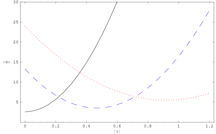
Figure 1: Mean photon number $\langle n\rangle$ as function of $|\gamma|$, for a HOMPSS with magnitude of squeezing $r=0.8$, coherent squeezed amplitude $\beta=3$, and different mixing angles: $\theta=0$ (full line); $\theta=\frac{\pi}{6}$ (dashed line); and $\theta=\frac{\pi}{4}$ (dotted line).

Due to the canonical condition $\phi=2\theta$, there cannot be pure squeezing for $\theta\neq 0$ even in absence of the nonlinearity, and thus at $\gamma=0$ we have different initial average numbers of photons depending on the value of $\theta$. The analytic expression for $\langle n\rangle$ for a homodyne transformation with $|\gamma|=0$ and $\phi=2\theta$ reads:

$$\langle n\rangle=|\beta|^{2}\cosh 2r-Re[\beta^{*2}e^{2\imath\theta}]\sinh 2r+\sinh^{2}r\;.$$ (42)

We see from Fig. 1 that $\langle n\rangle$ needs not show a monotonic behavior as a function of the nonlinearity. It is in fact very sensitive to the mixing angle $\theta$, and although it eventually always grows for sufficiently large values of $|\gamma|$, it can however initially decrease, depending on the mixing angle $\theta$, and then increasing again very slowly at larger values of $|\gamma|$. This behavior suggests that $\langle n\rangle$ will show even more remarkable properties when varying $\theta$ for different, fixed values of $|\gamma|$. In Fig. 2 we analyze the behavior of $\langle n\rangle$ as function of $\theta$, at fixed $|\gamma|$.

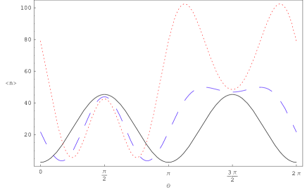
Figure 2: The mean photon number $\langle n\rangle$ as a function of $\theta$, for a HOMPSS with $r=0.8$, $\beta=3$ and different strengths of the nonlinearity: $|\gamma|=0$ (full line); $|\gamma|=0.5$ (dashed line); and $|\gamma|=1$ (dotted line).

For $|\gamma|=0$ we recover the oscillatory behavior of $\langle n\rangle$ as a function of the squeezing phase $\phi=2\theta$ of the standard two–photon squeezed state. When letting $\theta$ vary at fixed finite values of $|\gamma|$, the oscillations of $\langle n\rangle$ become faster, and both peaks and bottoms quickly rise to very large values. Therefore the nonlinearity plays the role of a “quantum coherent pump” allowing for very large average numbers of photons even in the case of lowest, quadratic nonlinearity.

V.3 Quasi–probability distributions and phase–space analysis

We now turn to the study of the statistics of direct, heterodyne, and homodyne detection for the homodyne multiphoton squeezed states $|\Psi\rangle_{\beta}$, showing in particular how the statistics is significantly modified by the tuning of the mixing angle $\theta$. We will consider the HOMPSS Eq. (26), corresponding to the canonical conditions Eqs. (9), and we will specialize to the lowest nonlinear function $F(x_{\theta})=x_{\theta}^{2}$.

We first consider the quasi–probability distributions associated to HOMPSS for some values of $\theta$ and compare them to the corresponding distributions associated to the standard two–photon squeezed states. This will allow a better understanding of the behavior of the photon number distributions and of the normalized correlation functions that will be computed later. The $Q$-function

$$Q(\alpha)=\frac{1}{\pi}|<\alpha|\Psi>_{\beta}|^{2}\;.$$ (43)

gives the statistics of heterodyne detection, and corresponds to a measure of two orthogonal quadrature components ($|\alpha\rangle$ being the coherent state associated to the coherent amplitude $\alpha=\alpha_{1}+i\alpha_{2}$). Figs. 3 and 4 show three–dimensional plots of the $Q-$function of the HOMPSS, for fixed values of $r$, $|\gamma|$, $\beta$ and for two different values of $\theta$.

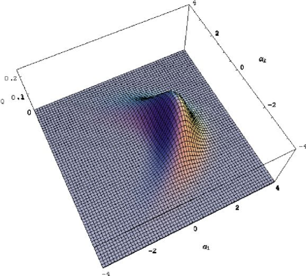
Figure 3: Plot of the $Q-$function, with $r=0.8$, $|\gamma|=0.4$, $\beta=3$, $\theta=\frac{\pi}{2}$, for the canonical conditions $\delta-\theta=-\frac{\pi}{2}$, $\delta+\theta-\phi=\frac{\pi}{2}$.

For $\theta=\pi/2$, which corresponds to the case $F=X_{2}^{2}$, i.e. no mixing, the plot resembles the $Q-$function for a squeezed state, but we can observe a deformation of the basis, curved along the $Re[\alpha]=\alpha_{1}$ axis. For $\theta=\pi/3$, a case of true mixing of the field quadratures, the deformation becomes much more evident and the function is strongly rotated and elongated with respect to the $Q$-function of the two–photon squeezed state.

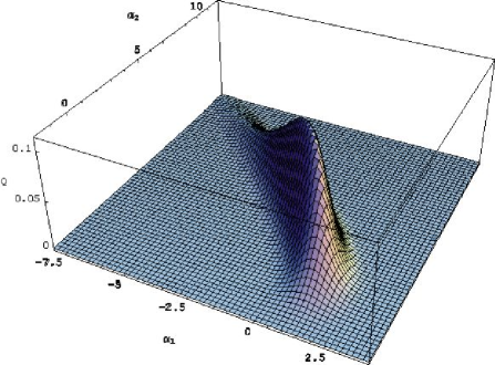
Figure 4: $Q-$function, with $r=0.8$, $|\gamma|=0.4$, $\beta=3$, $\theta=\frac{\pi}{3}$, for the canonical conditions $\delta-\theta=-\frac{\pi}{2}$, $\delta+\theta-\phi=\frac{\pi}{2}$.

Homodyne detection measures a quadrature component $X_{\lambda}=\frac{1}{\sqrt{2}}(a_{\lambda}+a_{\lambda}^{{\dagger}})$, where $\lambda$ is a phase determined by the phase of the local oscillator. Homodyne statistics correspond to project the Wigner quasiprobability distribution onto a $x_{\lambda}$ axis. With the identification $\lambda=\theta$ we plot the Wigner quasi–probability distribution for orthogonal quadrature components $x_{\theta}$ and $p_{\theta}$:

$$W(x_{\theta},p_{\theta})=\frac{1}{\pi}\int dye^{-2ip_{\theta}y}\Psi_{\beta}^{*}(x_{\theta}-y)\Psi_{\beta}(x_{\theta}+y)\;.$$ (44)

In Figs. 5 and 6 we show respectively a global projection and an orthogonal section of the Wigner function for $\theta=\pi/2$, i.e. no mixing, fixed canonical constraint, and intermediate value $|\gamma|=0.4$ of the nonlinearity.

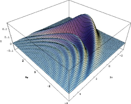
Figure 5: $W(x_{\theta},p_{\theta})$, with $r=0.8$, $|\gamma|=0.4$, $\beta=3$, $\theta=\frac{\pi}{2}$, for the canonical constraint $\delta-\theta=-\frac{\pi}{2}$, $\delta+\theta-\phi=\frac{\pi}{2}$.

We see from Figs. 5 and 6 that the Wigner function displays interference fringes and negative values, exhibiting a strong nonclassical behavior.

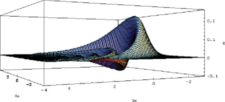
Figure 6: $W(x_{\theta},p_{\theta})$, with $r=0.8$, $|\gamma|=0.4$, $\beta=3$, $\theta=\frac{\pi}{2}$, for the canonical conditions $\delta-\theta=-\frac{\pi}{2}$, $\delta+\theta-\phi=\frac{\pi}{2}$.

In Fig. 7 we show the Wigner function, for the same values of $r$, $|\gamma|$, $\beta$, but for $\theta=\pi/3$, a value that realizes a true mixing of the field quadratures. We see that the distribution becomes strongly rotated and elongated, with a pattern of interference fringes and negative values, providing evidence of the complex statistical structure of the HOMPSS when a true homodyne mixing is realized.

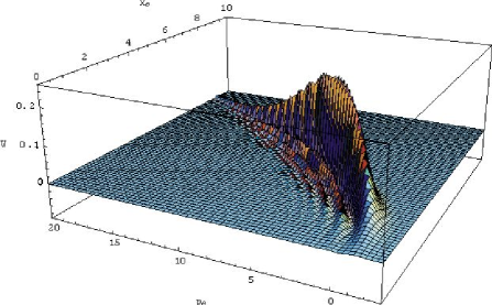
Figure 7: Plot of the Wigner function $W(x_{\theta},p_{\theta})$, with $r=0.8$, $|\gamma|=0.4$, $\beta=3$, $\theta=\frac{\pi}{3}$, for the canonical conditions $\delta-\theta=-\frac{\pi}{2}$, $\delta+\theta-\phi=\frac{\pi}{2}$.

The behaviors of the quasi–probability distributions suggest the following considerations. We recall that the HOMPSS, although being states of minimum uncertainty in the transformed (“dressed”) modes $(b,b^{\dagger})$, are not minimum uncertainty states for the original quadratures $X_{1}$ and $X_{2}$; in fact, Eqs. (39)–(41) show that a further term due to the unavoidable statistical correlations adds to the pure vacuum fluctuations. This fact is reflected in the rotation and in the deformation of the distributions. But we expect that this features will affect also the behavior of other statistical properties, like the photon number distribution. In particular, shape distortions of the quasi–probability distributions strongly modify the original ellipse associated to the standard two–photon squeezed states, giving rise, for suitable values of the parameters, to deformed intersection areas with the circular crowns associated in phase space to number states. In turn, this will lead to modified behaviors of the photon number distribution, including possible enhanced or subdued oscillations schleich as the mixing angle $\theta$ is varied. Moreover, we expect that also the second– and fourth– order normalized correlation functions will strongly depend on $\theta$, showing a deeper nonclassical behavior, for instance antibunching, in correspondence of values of $\theta$ associated to stronger nonclassical features of the Wigner function, like negative values and interference fringes.

V.4 Photon statistics

We begin by analyzing the probability for counting $n$ photons, the so-called photon number distribution (PND) $P(n)=|\langle n|\Psi\rangle_{\beta}|^{2}$, in direct detection, and neglecting detection losses:

$$P(n) = \left|\int dx_{\theta}\langle n|x_{\theta}\rangle\langle x_{\theta}|\Psi\rangle_{\beta}\right|^{2}$$ (45)

$$= \frac{1}{2^{n}n!\pi^{1/2}}\left|\int dx_{\theta}e^{-\frac{x_{\theta}^{2}}{2}}H_{n}(x_{\theta})\Psi_{\beta}(x_{\theta})\right|^{2}.$$

Due to the nonlinear nature of the function $F$, it is in general impossible to write a closed analytic expression for $P(n)$, which can however be easily determined numerically. In Fig. 8 we plot the PND of the HOMPSS for various intermediate values of the local oscillator $\theta$, together with the PND of the standard two–photon squeezed states.

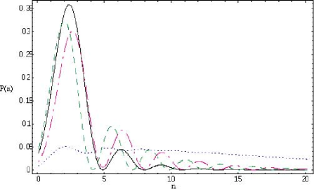
Figure 8: $P(n)$ for the HOMPSS, corresponding to the canonical constraints $\delta-\theta=-\frac{\pi}{2}$, $\delta+\theta-\phi=-\frac{\pi}{2}$, for different values of the parameters: $\beta=3$, squeezing magnitude $r=0.8$, and strength of the nonlinearity $|\gamma|=0$ (solid line); $\beta=3$, $r=0.8$, $|\gamma|=0.4$, $\theta=0$ (dotted line); $\beta=3$, $r=0.8$, $|\gamma|=0.5$, $\theta=\frac{\pi}{6}$ (dashed line); $\beta=3$, $r=0.5$, $|\gamma|=0.5$, $\theta=\frac{\pi}{4}$ (dot–dashed line).

As foreseen from the previous phase–space analysis, the behavior of the PND strongly depends on the value of the mixing angle $\theta$, and for suitable choices of $\theta$, $r$ and $|\gamma|$, the PND shows larger oscillations with respect to the standard two–photon squeezed states and the HOMPSS with $\theta=0$. Moreover, the oscillation peaks persist for growing $n$ and are shifted for different values of $|\gamma|$; this behavior is due to the different terms entering in the unitary operator $U_{\theta}(X_{\theta})$ Eq. (LABEL:Uph3), which mix in a peculiar way the quadrature operators for $\theta\neq 0,\pi/2$.

Concerning the correlation functions, it is interesting to study the behavior of the normalized second order correlation function

$$g^{(2)}(0)=\frac{\langle a^{{\dagger}2}a^{2}\rangle}{\langle a^{{\dagger}}a\rangle^{2}}=\frac{\langle a_{\theta}^{{\dagger}2}a_{\theta}^{2}\rangle}{\langle a_{\theta}^{{\dagger}}a_{\theta}\rangle^{2}}\;,$$ (46)

and of the normalized fourth order correlation function

$$g^{(4)}(0)=\frac{\langle a_{\theta}^{{\dagger}4}a_{\theta}^{4}\rangle}{\langle a_{\theta}^{{\dagger}}a_{\theta}\rangle^{4}}\;,$$ (47)

for the HOMPSS, and determine the different physical regimes. In Figs. 9 and 10 we compare $g^{(2)}(0)$ as a function of the squeezing parameter $r$ for the two–photon squeezed state and for the HOMPSS at different values of $\theta$.

Figure 9: The correlation function $g^{(2)}$ as function of $r$ for the HOMPSS, corresponding to the canonical constraints $\delta-\theta=-\frac{\pi}{2}$, $\delta+\theta-\phi=-\frac{\pi}{2}$, for several choices of the parameters: $\beta=3$, $\gamma=0$ (solid line); $\beta=3$, $|\gamma|=0.4$, $\theta=0$ (dashed line); $\beta=3$, $|\gamma|=0.05$, $\theta=\frac{\pi}{6}$ (dot–dashed line); $\beta=3$, $|\gamma|=0.5$, $\theta=\frac{\pi}{6}$ (dotted line).

Figure 10: The correlation function $g^{(2)}$ as function of $r$ for the HOMPSS, corresponding to the canonical conditions $\delta-\theta=-\frac{\pi}{2}$, $\delta+\theta-\phi=\frac{\pi}{2}$, versus the two-photon squeezed states (full line), for different choices of the parameters: 1) $\beta=3$, $|\gamma|=0.05$, $\theta=\frac{4\pi}{9}$ (dashed line); 2) $\beta=3$, $|\gamma|=0.2$, $\theta=\frac{\pi}{3}$ (dot-dashed line); 3) $\beta=3$, $|\gamma|=0.5$, $\theta=\frac{\pi}{3}$ (dotted line).

We see that also the correlation function $g^{(2)}(0)$ shows the strong nonclassical features of the HOMPSS; both the nonlinearity strength $|\gamma|$ and angle $\theta$ strongly influence the behavior of the curves. In fact, the curves deviate from the standard form and saturate at lower values with respect to TCS.

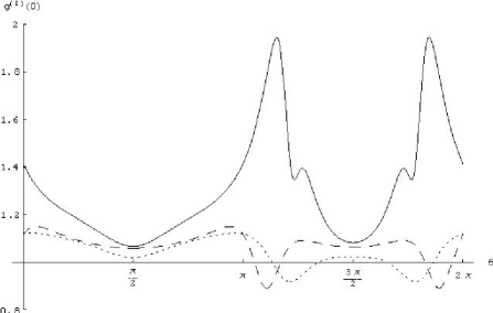
Figure 11: The correlation function $g^{(2)}$ as function of $\theta$ for the HOMPSS, corresponding to the canonical conditions $\delta-\theta=\frac{\pi}{2}$, $\delta+\theta-\phi=\frac{\pi}{2}$, for: 1) $\beta=3$, $r=0.5$, $|\gamma|=0.4$ (full line); 2) $\beta=3$, $r=0.4$, $|\gamma|=0.1$ (dashed line); 3) $\beta=3$, $r=0.1$, $|\gamma|=0.1$ (dotted line).

The most significant feature is however obtained plotting $g^{(2)}(0)$ as a function of $\theta$, Fig. 11, Fig. 12; the plots clearly demonstrate that it is possible to pass from a subpoissonian to superpoissonian statistics. So, tuning $\theta$, we can have photon bunching or antibunching and we can select the preferred statistics.

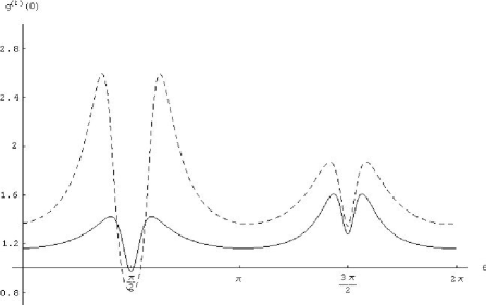
Figure 12: The correlation function $g^{(2)}$ as function of $\theta$ for the HOMPSS, corresponding to the canonical conditions $\delta-\theta=-\frac{\pi}{2}$, $\delta+\theta-\phi=\frac{\pi}{2}$, for: 1) $\beta=3$, $r=0.8$, $|\gamma|=0.1$ (full line); 2) $\beta=3$, $r=0.5$, $|\gamma|=0.4$ (dashed line).

Similar considerations can be made about the fourth order correlation function $g^{4}(0)$, as it can be seen by Fig. 13, where it is shown the dependence from the squeezing parameter $r$, and by Fig. 14, where instead $g^{4}(0)$ is plotted as a function of the angle $\theta$. Also the normalized fourth–order correlation function shows a particular shape for intermediate value of $\theta$ and varying saturation levels, depending on the parameters of the nonlinear term. Moreover, we have four photon bunching or anti-bunching in correspondence of different values of $\theta$.

Figure 13: The correlation function $g^{(4)}$ as function of $r$ for the HOMPSS, corresponding to the canonical conditions $\delta-\theta=-\frac{\pi}{2}$, $\delta+\theta-\phi=-\frac{\pi}{2}$, versus the two-photon squeezed states (full line), for several choices of the parameters: 1) $\beta=3$, $|\gamma|=0.4$, $\theta=0$ (dashed line); 2) $\beta=3$, $|\gamma|=0.4$, $\theta=\frac{\pi}{12}$ (dot-dashed line); 3) $\beta=3$, $|\gamma|=0.4$, $\theta=\frac{\pi}{6}$ (dotted line).

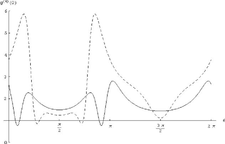
Figure 14: The correlation function $g^{(4)}$ as function of $\theta$ for the HOMPSS, corresponding to the canonical conditions $\delta-\theta=-\frac{\pi}{2}$, $\delta+\theta-\phi=-\frac{\pi}{2}$, for: 1) $\beta=3$, $r=0.5$, $|\gamma|=0.1$ (full line); 2) $\beta=3$, $r=0.1$, $|\gamma|=0.2$ (dashed line).

VI Conclusions and outlook

We have introduced single-mode nonlinear canonical transformations, which represent a general and simple extension of the linear Bogoliubov transformations. They are realized by adding a largely arbitrary nonlinear function of the homodyne quadratures $X_{\theta},P_{\theta}$. We have introduced the Homodyne Multiphoton Squeezed States (HOMPSS) defined as the eigenstates of the transformed annihilation operator. The HOMPSS are in general non Gaussian, higly nonclassical states which retain many properties of the standard coherent and squeezed states; in particular, they constitute an overcomplete basis in Hilbert space. On the other hand, many of their statistical properties can differ crucially from the ones of the Gaussian states. In particular, we have shown the strong dependence of the photon statistics on the local oscillator angle $\theta$. Among other remarkable features, there are the possibilities of exploiting the homodyne angle as a tuner to select sub–poissonian or super–poissonian statistics, and as catalyzer enhancing the average photon number in a state.

The single–mode multiphoton canonical formalism selects a large number of non Gaussian, nonclassical states, including the single–mode cubic phase state, which generalize the degenerate, Gaussian squeezed states. On the other hand, both from the point of view of modern applications, as e.g. quantum computation, and for experimental implementations, generalizations to two and many modes are of great interest.

In the following companion paper, ”Structure of multiphoton quantum optics. II. Bipartite systems, physical processes, and heterodyne squeezed states” (Part II), we will extend the canonical scheme developed in the present paper (Part I) to study multiphoton processes and multiphoton squeezed states for systems of two correlated modes of the electromagnetic field. This extension is important and desirable in view of the modern developments in the theory of quantum entanglement and quantum information. In particular, we will show how to define two-mode nonlinear canonical transformations and we will determine the associated “heterodyne multiphoton squeezed states” (HEMPSS). In the context of macroscopic (quantum) electrodynamics in nonlinear media, we will moreover discuss the kinds of multiphoton processes that can allow the experimental realizability of the HEMPSS and of the effective interactions associated to the two–mode nonlinear canonical formalism.

References

- (1) I. Bloch, M. Köhl, M. Greiner, T. W. Hänsch, and T. Esslinger, Phys. Rev. Lett. 87, 030401 (2001).
- (2) F. Dalfovo, S. Giorgini, L. Pitaevskii, and S. Stringari, Rev. Mod. Phys. 71, 463 (1999); A. J. Leggett, ibid. 73, 307 (2001).
- (3) I. L. Chuang and M. A. Nielsen, Quantum Computation and Quantum Information (Cambridge University Press, Cambridge, 2000); Fundamentals of Quantum Information, D. Heiss Ed. (Springer–Verlag, Berlin Heidelberg, 2002).
- (4) D. Stoler, Phys. Rev. D 4, 2309 (1971).
- (5) H. P. Yuen, Phys. Rev. A 13, 2226 (1976).
- (6) C. M. Caves and B. L. Schumaker, Phys. Rev. A 31, 3068 (1985); B. L. Schumaker and C. M. Caves, Phys. Rev. A 31, 3093 (1985).
- (7) R. J. Glauber, Phys. Rev. 131, 2766 (1963); Coherent States: Applications in Physics and Mathematical Physics, J. R. Klauder and B. S. Skagerstam Eds. (World Scientific, Singapore, 1985).
- (8) B. R. Mollow and R. J. Glauber, Phys. Rev. 160, 1076 (1967); L.–A. Wu, H. J. Kimble, J. L. Hall, and H. Wu, Phys. Rev. Lett. 57, 2520 (1986).
- (9) H. P. Yuen and J. H. Shapiro, IEEE Trans. Inf. Theory 24, 657 (1978).
- (10) C. M. Caves, K. S. Thorne, R. W. P. Drever, V. D. Sandberg and M. Zimmermann, Rev. Mod. Phys. 52, 341 (1980); C. M. Caves, Phys. Rev. D 23, 1693 (1981).
- (11) D. Gottesman, A. Kitaev and J. Preskill, Phys. Rev. A 64, 012310 (2001).
- (12) S. D. Bartlett and B. C. Sanders, Phys. Rev. A 65, 042304 (2002).
- (13) N. Bloembergen, Nonlinear Optics (Benjamin, New York, 1965); R. W. Boyd, Nonlinear Optics (Academic Press, 2002).
- (14) M. Brune et al., Phys. Rev. A 45, 5193 (1992); S. E. Harris, J. E. Field and A. Imamoglu, Phys. Rev. Lett. 64, 1107 (1990); M. D. Lukin and A. Imamoglu, Nature 413, 273 (2001); S. E. Harris and L. V. Hau, Phys. Rev. Lett. 82, 4611 (1999); A. B. Matsko, I. Novikova, G. R. Welch and M. S. Zubairy, LANL preprint quant–ph/0207141 (2002).
- (15) S. L. Braunstein and R. I. McLachlan, Phys. Rev. A 35, 1659 (1987); S. L. Braunstein and C. M. Caves, Phys. Rev. A 42, 4115 (1990).
- (16) G. D’Ariano, M. Rasetti and M. Vadacchino, Phys. Rev. D 32, 1034 (1985); J. Katriel, A. I. Solomon, G. D’Ariano, and M. Rasetti, Phys. Rev. D 34, 2332 (1986); G. D’Ariano, M. Rasetti, Phys. Rev. D 35, 1239 (1987).
- (17) S. De Siena, A. Di Lisi, and F. Illuminati, Phys. Rev. A 64, 063803 (2001).
- (18) S. De Siena, A. Di Lisi, and F. Illuminati, J. Phys. B: At. Mol. Opt. Phys. 35, L291 (2002).
- (19) Y. Wu and R. Côté, Phys. Rev. A 66, 025801 (2002).
- (20) P. G. Kwiat, K. Mattle, H. Weinfurter, A. Zeilinger, A. V. Sergienko, and Y. Shih, Phys. Rev. Lett. 75, 4337 (1995); Z. Y. Ou, J. K. Rhee and L. J. Wang, Phys. Rev. A 60, 593 (1999); J.–W. Pan, M. Daniell, S. Gasparoni, G. Weihs and A. Zeilinger, Phys. Rev. Lett. 86, 4435 (2001); H. Weinfurter and M. Zukowski, Phys. Rev. A 64, 010102(R) (2001).
- (21) F. Dell’Anno, S. De Siena, and F. Illuminati, “Structure of multiphoton quantum optics. II. Bipartite systems, physical processes, and heterodyne squeezed states”, LANL preprint quant–ph/0308094 (2003).
- (22) W. Schleich and J. A. Wheeler, Nature (London) 326, 574 (1987); W. Schleich, D. F. Walls and J. A. Wheeler, Phys. Rev. A 38, 1177 (1988).