Correlated motion of two atoms trapped in a single mode cavity field

Abstract

We study the motion of two atoms trapped at distant positions in the field of a driven standing wave high $Q$ optical resonator. Even without any direct atom-atom interaction the atoms are coupled through their position dependent influence on the intracavity field. For sufficiently good trapping and low cavity losses the atomic motion becomes significantly correlated and the two particles oscillate in their wells preferentially with a $90^{\circ}$ relative phase shift. The onset of correlations seriously limits cavity cooling efficiency, raising the achievable temperature to the Doppler limit. The physical origin of the correlation can be traced back to a cavity mediated cross-friction, i.e. a friction force on one particle depending on the velocity of the second particle. Choosing appropriate operating conditions allows for engineering these long range correlations. In addition this cross-friction effect can provide a basis for sympathetic cooling of distant trapped clouds.

I Introduction

It is a well established fact, both theoretically and experimentally, that light forces on atoms are substantially modified within resonant optical cavities domokos03 ; vuletic01 ; vanenk01 ; munstermann00 ; kruse03 ; doherty97 ; mossberg91 ; rempe04 . Possible experimental realizations range from single atoms or ions mundt02 ; guthohrlein02 in microscopic super cavities to several thousand vuletic03a ; chapman03 or up to a million atoms kruse03 ; zimmermann03 in a high $Q$ ring cavity. Applications of these systems include possible implementations of quantum information processing setups hemmerich99 ; griessner03 , and controlled nonclassical light sources kimble03 ; kuhn02 as well as new possibilities for trapping and cooling of atoms and molecules. The basic physical mechanism in these setups can be traced back to the backaction of the atoms on the field. They act as a moving refractive index and absorber, modifying the intensity and phase of the intracavity field, which in turn governs their motion. This coupled dynamics is at the heart of cavity enhanced trapping and cooling.

It is clear that if a single atom is able to change the field, it will influence other atoms in the same field irrespective of their distance. This introduces long range atom-atom interactions, which are widely tailorable by suitable choices of cavity geometries and operating conditions. On one hand these interactions are useful and can be used to implement bipartite quantum gates hemmerich99 . On the other hand they play a decisive role in the scaling properties of cavity enhanced cooling horak01 ; fischer01 . For perfectly correlated atoms, the change of refractive index induced by one atom can be compensated by a second atom, so that the effective atom-field back reaction can be strongly reduced. For several atoms in a ring cavity this effect only allows a weak damping of relative motion, while the center of mass motion is strongly damped gangl00b . This model is closely related to the so-called CARL laser, where the kinetic energy of an atomic beam leads to gain into the counterpropagating mode of a single side pumped ring resonator bonifacio97 . New effects were also found in the study of the coupling of two Bose-condensates in a cavity jaksch01 .

Several limiting cases for N atoms commonly interacting with a cavity mode have already been studied. For the case of N strongly trapped atoms in a standing wave cavity mode, it is possible to derive a set of coupled equations for the total kinetic and potential energy as well as the field amplitude gangl99 , which exhibit collective, damped oscillations ending in highly correlated steady states. This approach, however, does not give much insight into the details of the individual dynamics and correlations. In the opposite limit of N untrapped atoms moving in the cavity field, numerical simulations show little influence of atom-atom correlations and cooling proceeds independent of the atom number horak01 for proper rescaling of the cavity parameters.

Recently an approach for several atoms in a single mode cavity has been developed, which concentrates on the effect of the $N-1$ other particles on the cooling properties of a single one fischer01 . This, in principle, makes it possible to study the combined optical potential and friction forces. It has been recently proposed theoretically domokos02b and confirmed experimentally vuletic03 , that if the atoms are pumped directly from the side (as opposed to pumping the cavity), the buildup of spatial correlations within a cloud of trapped atoms can lead to superradiant light scattering and enhanced cooling behavior. The theoretical results in this case are based on numerical simulations of the semiclassical equations of motion for a large number $N\gg 1$ of particles domokos02b . This clearly demonstrates collective effects, but does not give much quantitative insight in the buildup and role of atom-atom correlations.

The central goal of the present work is to study the basic physical mechanisms responsible for the motional correlations and to develop quantitative measures of the established steady state correlation. For this we restrict ourselves to the simplest nontrivial example, namely two atoms strongly coupled to a single standing wave field of a cavity. The energy loss is compensated by cavity pumping, and large detuning from the atomic transition is taken to ensure low atomic saturation. Moreover, the motion of the atoms is only followed along the cavity axis. As we will see, this contains most of the essential physics but still allows us to derive analytical expressions for many relevant quantities. Most of the analytical results are valid for the more general $N$-atom case.

The article is organized as follows: after presenting our model and the approximations used in section II, we analytically discuss the central physical mechanisms present in section III. In section IV we quantify the results using numerical simulations, which are then analyzed in more detail in section V.

II The model

Let us start by outlining the system which is shown in Fig. 1. We consider $N=2$ two-level atoms with transition frequency $\omega_{A}$ strongly coupled to a single mode of a high-finesse cavity with frequency $\omega_{C}$. The system is driven by a coherent laser field of frequency $\omega$ and amplitude $\eta$ injected into the cavity through one of the mirrors. The model and its theoretical treatment follow closely Ref. domokos03 . Coupling to the environment introduces a damping via two channels. First, the atoms spontaneously emit with a rate of $2\gamma$ into the vacuum outside the cavity. Second, the cavity photons decay with rate $2\,\kappa$ via the output coupler mirror of the cavity. The atoms can move freely in the cavity, however, for the sake of simplicity, their motion is restricted to the cavity axis (dashed line in Fig. 1).

Figure 1: The setup. The motion of two two-level atoms in a far-detuned, high-Q optical cavity is studied. The cavity is pumped by a strong laser beam, almost on resonance with the cavity mode. Atomic motion is discussed along the cavity axis only.

Applying the standard Born-Markov approximation the dynamics are governed by a quantum master equation,

$$\dot{\rho}=-\frac{i}{\hbar}[\hat{H},\rho]+\cal L\rho.$$ (1)

Using rotating-wave and dipole approximations the Hamiltonian and the Liouville operators in an interaction picture read domokos03 :

$$\hat{H} =\sum_{k=1}^{N}\left[\frac{\hat{\mathbf{p}}_{k}^{2}}{2m}-\hbar\Delta_{A}\hat{\sigma}_{k}^{z}\right]$$

$$\quad-\hbar\Delta_{c}\hat{a}^{\dagger}\hat{a}-i\hbar\eta\left(\hat{a}-\hat{a}^{\dagger}\right)\;$$

$$\quad-i\hbar\sum_{k=1}^{N}\left(g(\hat{\mathbf{x}}_{k})\hat{\sigma}_{k}^{\dagger}\hat{a}-g^{*}(\hat{\mathbf{x}}_{k})\hat{a}^{\dagger}\hat{\sigma}_{k}\right)$$ (2a)

$${\cal L}\hat{\varrho} =\kappa\left(2\hat{a}\hat{\varrho}\hat{a}^{\dagger}-\hat{a}^{\dagger}\hat{a}\hat{\varrho}-\hat{\varrho}\hat{a}^{\dagger}\hat{a}\right)$$

$$\quad+\gamma\sum_{k=1}^{N}\Bigl{(}2\int d^{2}{\mathbf{u}}\;N({\mathbf{u}})\hat{\sigma}_{k}e^{-ik_{A}{\mathbf{u}}\hat{\mathbf{x}}_{k}}\hat{\varrho}e^{ik_{A}{\mathbf{u}}\hat{\mathbf{x}}_{k}}\hat{\sigma}_{k}^{\dagger}$$

$$\quad-\hat{\sigma}_{k}^{\dagger}\hat{\sigma}_{k}\hat{\varrho}-\hat{\varrho}\hat{\sigma}_{k}^{\dagger}\hat{\sigma}_{k}\Bigr{)}\,.$$ (2b)

The atomic and cavity field detunings are defined as $\Delta_{A}=\omega-\omega_{A}$ and $\Delta_{C}=\omega-\omega_{C}$, respectively. The annihilation and creation operators of the cavity field are $\hat{a}$ and $\hat{a}^{\dagger}$, while $\hat{\sigma}_{k}$ and $\hat{\sigma}_{k}^{\dagger}$ are the lowering and raising operators of the $k$-th atom. The Hamiltonian consists of the motional and internal energy of the atoms, the self-energy of the cavity field, the classical (laser) pump, and the Jaynes–Cummings-type interaction between the atoms and the field. The position dependence of the coupling constant is due to the spatial structure of the field mode: $g(\mathbf{x}_{k})=g_{0}f(\mathbf{x}_{k})$, where in our standing-wave cavity $f(\mathbf{x}_{k})=\cos(k_{C}x_{k})$, with $k_{C}=2\pi/\lambda$ being the cavity wavenumber. The Liouvillean operator includes the effect of cavity losses and of the spontaneous emissions on the combined atom-cavity field density operator $\hat{\varrho}$. This latter is given by the last term, where the integral goes over the directions of photons spontaneously emitted by the atomic dipole, having expected wavenumber $k_{A}=\omega_{A}/c$ and angular distribution $N(\mathbf{u})$.

We consider cold atoms but with a temperature well above the recoil limit $k_{B}T_{rec}=\hbar k_{A}^{2}/(2M)$, where $M$ is the mass of one atom. In this limit the atomic coherence length is smaller than the optical wavelength and the position and momentum of the atoms can be replaced by their expectation values and treated as classical variables. We still keep the quantum nature of the internal variables $\hat{a}$ and $\hat{\sigma}_{k}$. Moreover, if the atoms move much less than a wavelength during the equilibration time of the internal variables

$$v\ll\lambda\kappa,\lambda\gamma,$$ (3)

we can adiabatically separate the ”fast” internal from the ”slow” external dynamics as in standard laser cooling models domokos02 .

II.1 The internal dynamics

For given positions of the atoms $\mathbf{x}_{k}$ the internal atomic dynamics can be rewritten in the form of quantum Langevin equations. For low saturation, i.e. when $\left\langle{\hat{\sigma}^{\dagger}\hat{\sigma}}\right\rangle\ll 1$, we can approximate the operator $\hat{\sigma}_{z}$ by $-1/2$ (this is called bosonization of the atomic operators). The resulting Heisenberg–Langevin equations then reduce to the following set of coupled linear differential equations:

$$\frac{\mathrm{d}}{\mathrm{d}t}{\hat{a}} =(i\Delta_{C}-\kappa)a+\sum_{k}g^{*}({\mathbf{x}}_{k})\hat{\sigma}_{k}+\eta+\hat{\xi}$$ (4a)

$$\frac{\mathrm{d}}{\mathrm{d}t}{\hat{\sigma}}_{k} =(i\Delta_{A}-\gamma)\hat{\sigma}_{k}-g({\mathbf{x}}_{k})\hat{a}+\hat{\zeta}_{k}.$$ (4b)

The noise operators $\hat{\xi}$ and $\hat{\zeta}_{k}$ appear as a result of the coupling to the external vacuum through the cavity mirrors and through spontaneous emission. They contain the annihilation operators of the external vacuum modes, and therefore give $0$ when acting on the environment’s state. Their second-order correlation functions are as follows:

$$\langle\hat{\xi}(t_{1})\hat{\xi}^{+}(t_{2})\rangle =2\kappa\,\delta(t_{1}-t_{2}),$$ (5a)

$$\langle\hat{\zeta}_{k}(t_{1})\hat{\zeta}^{+}_{m}(t_{2})\rangle =2\gamma\,\delta_{km}\delta(t_{1}-t_{2}),$$ (5b)

while all other correlations vanish.

The steady state expectation values of the internal variables $\hat{a}$ and $\hat{\sigma}_{k}$ obtained from the Heisenberg–Langevin equations (4) then read:

$$\left\langle{\hat{a}}\right\rangle =\eta\frac{\gamma-i\Delta_{A}}{\mathcal{D}^{\prime}}$$ (6a)

$$\left\langle{\hat{\sigma}_{l}}\right\rangle =-\eta\frac{g(\mathbf{x}_{l})}{\mathcal{D}^{\prime}}.$$ (6b)

Here $\mathcal{D}^{\prime}$ is the reduced determinant of the Bloch matrix,

$$\mathcal{D}^{\prime}=(i\Delta_{C}-\kappa)(i\Delta_{A}-\gamma)+\sum_{l}g(\mathbf{x}_{l})^{2}.$$ (7)

Since the factor $1/\mathcal{D}^{\prime}$ appears in both expectation values and in later formulae as well, it is worthwhile to rewrite it to reveal its resonance structure with respect to the cavity detuning:

$$\frac{1}{\mathcal{D}^{\prime}} =\frac{1}{(i\Delta_{A}-\gamma)}\,\frac{1}{i(\Delta_{C}-U)-(\kappa+\Gamma)},$$ (8)

$$\mathrm{where}\qquad U=\frac{\Delta_{A}\sum_{l}g^{2}(\mathbf{x}_{l})}{\Delta_{A}^{2}+\gamma^{2}}=U_{0}\sum_{l}f^{2}(\mathbf{x}_{l}),$$ (9)

$$\mathrm{and}\qquad\quad\Gamma=\frac{\gamma\sum_{l}g^{2}(\mathbf{x}_{l})}{\Delta_{A}^{2}+\gamma^{2}}=\Gamma_{0}\sum_{l}f^{2}(\mathbf{x}_{l}),$$ (10)

and we used $g(x)=g_{0}f(x)$. It is clearly seen that each atom broadens the resonance at most by $\Gamma_{0}$ and displaces it by $U_{0}$.

II.2 The external dynamics

The motion of the atoms is governed by the force operator,

$$\begin{split}\hat{\mathbf{F}}_{k}=\frac{i}{\hbar}[\hat{p},\hat{H}]=i\hbar\left[\nabla g({\mathbf{x}}_{k})\,\hat{\sigma}_{k}^{\dagger}\hat{a}-\nabla g^{*}({\mathbf{x}}_{k})\,\hat{a}^{\dagger}\hat{\sigma}_{k}\right]\;.\end{split}$$ (11)

Since $\hat{\mathbf{F}}_{k}$ is normally ordered, its expectation value is easily obtained upon insertion of the stationary solution (6) of the internal variables. For a moving atom this expression is only approximately valid: there will be a time lag in the internal dynamics with respect to the atom’s current position, and hence we will include corrections to $\hat{\mathbf{F}}_{k}$ to first order in the atomic velocities.

The slow evolution of the centers of mass of the atoms, smoothed out on the timescale $\tau\approx\mathrm{max}\{1/\kappa,1/\gamma\}$ is described by the coupled Langevin equations:

$$\dot{\mathbf{x}}_{k} ={\mathbf{p}}_{k}/M,$$ (12a)

$$\dot{\mathbf{p}}_{k} ={\mathbf{f}}_{k}+\sum_{m=1}^{N}{\boldsymbol{\beta}}_{km}{\mathbf{p}}_{m}/M+{\boldsymbol{\Xi}}_{k}\;.$$ (12b)

In these equations ${\mathbf{f}}_{k}=\left\langle{\hat{\mathbf{F}}_{k}}\right\rangle$ are the vectors giving the steady state $v=0$ contribution of the force, while ${\boldsymbol{\beta}}_{km}$ are the tensors describing the first order corrections to the force acting on atom $k$. ${\boldsymbol{\Xi}}_{k}$ denotes the Langevin noise forces due to photon recoil. They correspond to random kicks along the cavity axis with zero average and second moments given by $\left\langle{{\boldsymbol{\Xi}}_{k}{\boldsymbol{\Xi}}_{m}}\right\rangle={\mathcal{D}}_{km}$. Note that the matrix ${\mathcal{D}}_{km}$, representing the strength of the Langevin noise, depends on the time-varying atomic positions. It represents the quantum fluctuations of the force due to the fact $\left\langle{\hat{F}_{k}\circ\hat{F}_{m}}\right\rangle\neq\left\langle{\hat{F}_{k}}\right\rangle\circ\left\langle{\hat{F}_{m}}\right\rangle$. It is by the addition of the noise terms ${\boldsymbol{\Xi}}_{k}$ that we tailor our classical force to give the same second-order expectation values as its quantum counterpartdomokos03 .

III Interaction channels

The Hamiltonian (2) contains no direct coupling between the two atoms: these only arise indirectly due to coupling to the same field mode. Interestingly the atom-atom interaction appears in all the three types of forces present in classical equations of motion (12). First, the steady state force $\mathbf{f}_{k}$ depends on the positions of both atoms via the steady state intensity. Second, not only does the friction coefficient on one atom depend on the position of the other, but the friction matrix has off-diagonal terms as well. This means that apart from ordinary viscous friction ($\dot{\mathbf{p}}_{k}\propto\mathbf{v}_{k}$) a strange phenomenon, which we call cross-friction ($\dot{\mathbf{p}}_{k}\propto\mathbf{v}_{l}$, for $l\neq k$) is also present. Here the velocity of one atom influences the friction experienced by the other atom. Third, the Langevin noise term on one atom has an expected magnitude influenced by the position of the other, and the noise terms ${\boldsymbol{\Xi}}_{k}$ are directly correlated as well. Hence we get joint “kicks” on both atoms leading to correlated motion. In the following we will analyze these interaction channels in more detail.

III.1 Steady state force $\mathbf{f}$

Formally the expectation value $\mathbf{f}_{k}$ of the force operator looks very similar to the case of free-space Doppler cooling:

$${\mathbf{f}}_{k}=-\hbar\frac{\Delta_{A}}{\Delta_{A}^{2}+\gamma^{2}}\left\langle{\hat{a}^{\dagger}\hat{a}}\right\rangle\mathbf{\nabla}_{k}g^{2}(\mathbf{x}_{k}).$$ (13)

However it additionally depends on the positions of the other atoms via the cavity field intensity. This dipole force is conservative and can be derived from a potential. The potential looks more complicated than in free space as it contains the dynamical nature of the cavity field, but still can be given in closed form fischer01 :

$$V=\frac{\hbar\Delta_{A}\left|{\eta}\right|^{2}}{\Delta_{A}\kappa+\Delta_{C}\gamma}\mathrm{atan}\frac{\gamma\kappa-\Delta_{A}\Delta_{C}+\sum_{l}{g^{2}(x_{l})}}{\Delta_{A}\kappa+\Delta_{C}\gamma}.$$ (14)

To show the effects of dynamic field adjustment, we plot this potential for two typical cases in Fig. 2. For the experimental parameters used in an experiment at MPQ in Garching fischer02 (Garching parameters), $\kappa=\gamma/2$, $g_{0}=5\gamma$, and for a detuning $\Delta_{A}=-50\gamma$ (upper graph) the effective interaction between the atoms is relatively weak and the potential resembles the familiar “egg-carton” surface proportional to $\sin^{2}(k_{C}x_{1})+\sin^{2}(k_{C}x_{2})$. For a somewhat stronger atom-field coupling $g_{0}=20\gamma$ (lower graph in Fig. 2) the atomic interaction is quite obvious and the shape of the potential of the second atom strongly depends on the position of the first atom and vice versa. Basically in this second case either both atoms are trapped, or both are free.

The peculiar $g_{0}$-dependence of the interaction and the trapping effects can be understood physically by looking at formula (13). The atoms see each other through the cavity field $\left\langle{\hat{a}^{\dagger}\hat{a}}\right\rangle$. As we saw in formulae (8,9,10), the field is in resonance when $U({\mathbf{x}}_{1},{\mathbf{x}}_{2})$ is approximately $\Delta_{C}\pm(\Gamma+\kappa)$. Each atom can shift $U$ in this far-detuned case by approximately $U_{0}\approx g_{0}^{2}/\Delta_{A}$, whereas the cavity linewidth is approximately $\kappa+\gamma g_{0}^{2}/\Delta_{A}^{2}$. Using the MPQ parameters $U_{0}<\kappa$, and therefore the back-action of the atoms on the cavity field is weak. In the large-$g_{0}$ case, $U_{0}>\kappa$, but $\Gamma_{0}<\kappa$, meaning that the atoms can shift the cavity resonance significantly more than a linewidth. Hence if one of the atoms leaves its trap it will shift the cavity out of resonance and cause the other atom to be released as well. Moreover, the amplitude of the force is proportional to the cavity field, which in the large-$g_{0}$ case decreases faster with the distance from the trapping point. This implies that less work needs to be done to free an atom: the potential is smaller, despite the same maximum light shift.

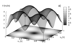
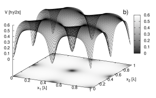
Figure 2: Potential as a function of atomic positions The potential (14) is plotted as a function of positions of the two atoms. In a) the Garching parameters ($\kappa=\gamma/2$,$g_{0}=5\gamma$) are used, in b) $g_{0}$ was increased fourfold. In the first case, the potential is well approximated by a sum of two single-particle potentials. In the second case, it is seen that either both atoms are trapped or both are free. The trap is deeper for smaller couplings.

Let us now analyze the interaction in a more quantitative way. We start from the limiting case of neglecting the atomic back-action on the field (i.e. we assume a constant field intensity). This corresponds to the force (13)

$${\mathbf{f}}_{l}\approx\frac{\hbar\left|{\eta}\right|^{2}}{2\Delta_{A}\kappa^{2}}\mathbf{\nabla}_{l}g^{2}(\mathbf{x}_{l})$$ (15)

one obtains in the limit of very large atom-field detuning. We can now find corrections from the cavity-mediated interaction to this force by expanding the potential (14) in a power series. Setting the driving field to resonance, $\Delta_{C}=U_{0}-\kappa$, the potential Eq. (14) to second order in ${\gamma}/{\Delta_{A}}$ reads

$$V\approx\frac{\hbar\left|{\eta}\right|^{2}}{\kappa}\left[\frac{\pi}{4}-\left(\left(1+\frac{\pi}{4}\right)+\frac{g_{0}^{2}}{2\kappa\gamma}\sum_{l=1}^{N}{f^{2}({x}_{l})}\right)\frac{\gamma}{\Delta_{A}}\right.\\ \left.+\Bigg{\{}\left(1+\frac{\pi}{4}\right)-\left(1+\frac{\pi}{2}\right)N\right.\\ \left.+\left(\frac{g_{0}^{2}}{2\kappa\gamma}\right)^{2}\bigg{(}\sum_{l=1}^{N}{f^{2}(x_{l})}\bigg{)}^{2}\Bigg{\}}\left(\frac{\gamma}{\Delta_{A}}\right)^{2}\right].$$ (16)

To first order in the small parameter we have a sum of single-atom potentials, giving the “egg-carton” shape. The corrections to this are given by terms of higher order in our expansion parameter, of which we give the first nontrivial term here. Note that since it is not simply the distance of the atoms upon which the potential depends, the interatomic force between them – as can be read out from the above formula – is not a “force” in the sense of Newton’s third law.

III.2 Forces linear in velocity: friction and cross-friction

To lowest order in the adiabatic separation of the internal and external dynamics we used the steady state values of the internal variables for fixed positions of the atoms to calculate the above potentials. As a next step we can include corrections for $\hat{a}$ and the $\hat{\sigma}_{k}$ linear in the velocity ${\mathbf{v}}_{m}$ of each atom, which should be valid for low velocities. As described in domokos03 this leads to a friction matrix ${\boldsymbol{\beta}}_{km}$ as first order correction to ${\mathbf{f}}_{k}$.

We obtain the following explicit formula for the friction matrix,

$${\boldsymbol{\beta}}_{km}=2\hbar\mathbf{\nabla}_{k}g(\mathbf{x}_{k})\circ\mathbf{\nabla}_{m}g(\mathbf{x}_{m})\frac{\eta^{2}}{\left|{\mathcal{D}^{\prime}}\right|^{2}}\gamma\frac{2\Delta_{A}}{\Delta_{A}^{2}+\gamma^{2}}\delta_{km}\\ +\hbar\mathbf{\nabla}_{k}g^{2}(\mathbf{x}_{k})\circ\mathbf{\nabla}_{m}g^{2}(\mathbf{x}_{m})\frac{\eta^{2}}{2\left|{\mathcal{D}^{\prime}}\right|^{2}}\Im\left\{\frac{1}{{\mathcal{D}^{\prime}}^{2}}\cdot\right.\\ \left.\left(2(1+\chi)\left((i\Delta_{A}-\gamma)^{2}-\sum_{l}g(\mathbf{x}_{l})^{2}\right)+(1+3\chi){\mathcal{D}^{\prime}}\right)\right\}$$ (17)

where $\chi=(i\Delta_{A}+\gamma)/(i\Delta_{A}-\gamma)$ is a complex factor of unit modulus, which for large atomic detuning, $\Delta_{A}\gg\gamma$, becomes approximately $\chi\approx 1$. This formula differs somewhat from that obtained by Fischer et al. fischer01 by a slightly different approach. The most important difference is that we find a matrix symmetric in the indices ${km}$. This is important because it is these off-diagonal terms that couple the velocities of the atoms, and have a decisive influence on the buildup of correlated motion. We defer detailed discussion of the formula (17) to Section V.

III.3 Random forces due to quantum noise

Spontaneous emission and cavity decay introduce quantum noise into the atomic motion. These heat up the system and generally tend to decrease motional correlations of the atoms. Following the line of reasoning briefly mentioned at the end of section II and discussed in more detail in domokos03 , we can calculate the influence of the noise operators $\hat{\xi}$ and $\hat{\zeta}$ of eq. (4) on the dynamics. For $N$ atoms we arrive at the following simple formula:

$${\mathcal{D}}_{km}=2\hbar^{2}\mathbf{\nabla}_{k}g(\mathbf{x}_{k})\circ\mathbf{\nabla}_{m}g(\mathbf{x}_{m})\frac{\eta^{2}}{\left|{\mathcal{D}^{\prime}}\right|^{2}}\gamma\delta_{km}\\ +2\hbar^{2}\mathbf{\nabla}_{k}g(\mathbf{x}_{k})^{2}\circ\mathbf{\nabla}_{m}g(\mathbf{x}_{m})^{2}\frac{\eta^{2}}{\left|{\mathcal{D}^{\prime}}\right|^{2}}\Delta_{A}\frac{\kappa\Delta_{A}+\gamma\Delta_{C}}{\left|{\mathcal{D}^{\prime}}\right|^{2}}.$$ (18)

This is a simple extension of the corresponding formula for one atom given in domokos03 . Let us remark here, that the diagonal part of this diffusion matrix ${\mathcal{D}}_{km}$ has been also found by Fischer et al. fischer01 . Surprisingly one also obtains off-diagonal terms, which have not been considered before. These terms lead to correlated kicks on the atoms, which can .add to the atom-atom correlations, rather than destroying them.

Spontaneous emission adds recoil noise, which gives an extra term to the noise correlation matrix of the form:

$${\mathcal{D}}^{\mathrm{sp}}_{km}=\delta_{km}2\hbar^{2}k_{A}^{2}\overline{u^{2}}\frac{\eta^{2}g(\mathbf{x})^{2}}{\left|{\mathcal{D}^{\prime}}\right|^{2}}\gamma.$$ (19)

Here $k_{A}=\omega_{A}/c$ is the expected wavenumber of the emitted photons and $\overline{u^{2}}$ is the correction factor coming from the spatial distribution of the photons, in our case $\overline{u^{2}}=2/5$. As expected, spontaneous emission, being a single-atom process, induces no correlations between the atoms.

IV Numerical simulations of the correlated atomic motion

Having discussed the qualitative nature of the combined atom field dynamics, we now turn to numerical simulations for some quantitative answers. We numerically integrate the Langevin equations (12), varying the ratio of the cavity loss rate to the linewidth of the atom $\kappa/\gamma$ as well as the relative coupling strength $g_{0}/\gamma$. Note that the relative magnitude of radiation pressure and dipole force can be changed by varying the detuning between pump frequency and the atomic resonance. As we are interested in cooling and trapping the atoms we fix the cavity frequency at $\Delta_{C}=NU_{0}-\kappa$ to ensure efficient cooling horak97 ; domokos03 . The pump power is always chosen to keep the atomic saturation low and approximately at ($\left\langle{\hat{\sigma}_{k}^{+}\hat{\sigma}_{k}}\right\rangle<0.1$) at all times.

Typical trajectories of atom pairs are shown in Figure 3.

Figure 3: Typical trajectories in coordinate space. In the left column, in a) and b), the parameters of the Garching group are used, in the right column, in c) and d), we considered a better resonator ($\kappa=0.1\gamma,g_{0}=10\gamma$) and larger detuning ($\Delta_{A}=-10000\gamma$). In both cases the first $50\mu\mathrm{s}$, in a) and c), and the first $3\mathrm{ms}$, in b) and d), are shown. The coordinate is the distance from the nearest trappping point.

The atomic positions $\big{(}x_{1}(t_{n}),x_{2}(t_{n})\big{)}$ are plotted at regular time intervals $t_{n}$. For better visibility the coordinate is always measured from the nearest trapping point. In the left column the detuning was chosen ($\Delta_{A}=-50\gamma$), with the cavity parameters of the MPQ group at Garching fischer02 ($\kappa=\gamma/2$, $g_{0}=5\gamma$). The first $50\mu\mathrm{s}$ are displayed in the figure on the top, and the first $3\mathrm{ms}$ in the one on the bottom. Both atoms localize during the first $50\mu\mathrm{s}$ to within 1/4 of a wavelength around respective trapping centers, a sign of cooling and trapping by the cavity. In the right column, the detuning is chosen much larger ($\Delta_{A}=-10^{4}\gamma$) with stronger atom-field coupling ($\kappa=\gamma/10$, $g_{0}=10\gamma$). In this case the relative importance of spontaneous emission is strongly reduced. The cooling in the cavity is faster and both atoms reach a steady state rapidly.

The appearance of a circular structure is the striking feature of the right column. This indicates that the motion of the atoms is correlated. Both atoms move sinusoidally about their respective trapping points, with some noise but in such a way that the relative phase of the two oscillations is likely to be $+90^{\circ}$ or $-90^{\circ}$.

To quantify the correlation between the atomic oscillators we define their oscillator phases. This is computed in the simulation using the trap frequency, which is:

$$\omega_{\mathrm{trap}}=\sqrt{2\hbar\left|\Delta_{A}\right|\left\langle{\hat{\sigma}^{\dagger}\hat{\sigma}}\right\rangle k_{C}^{2}/M},$$ (20)

if both atoms are well trapped. Here $k_{C}$ is the resonator mode wavenumber, and $\left\langle{\hat{\sigma}^{\dagger}\hat{\sigma}}\right\rangle$ is the saturation of either atom at the trapping point. This formula can be derived by expanding the potential (14), and substituting our particular choice of $\eta$ and $\Delta_{C}$.

The measured time evolution of the oscillator phases for the MPQ parameters (left column) and the “improved” parameters (right column) are shown in Fig. 4.

Figure 4: The phases of the atomic oscillations and the relative phase. The time evolution of the oscillator phases of the first (upper row) and second (middle row) atoms is shown, with the phase difference (bottom row). On the left the parameter set of the Garching experiments is used, on the right a better cavity is taken with larger atomic detuning, as in the text. The phases of the atoms evolve too fast on this timescale, only noise is seen. The phase difference is slower, with the ”improved” parameter set it appears to stabilize at $+90^{\circ}$ and $-90^{\circ}$.

For each parameter set, representative runs shown in Fig. 3 are used, and the oscillator phases of atom 1 (upper row), atom 2 (middle row) and the phase difference (lower row) are displayed. The rapid oscillation of the atoms (the period is $2.9\ \mu$s for the Garching parameters and $0.17\ \mu$s for the idealized ones) means that the time evolution of the phases is too fast to be followed on the timescale shown, in the upper and middle rows only “noise” is seen. The phase difference, however, evolves more slowly. This effect is more pronounced for the second parameter set, where the dipole force dominates. Moreover, in this second case, the phase difference clearly stabilizes around $+90^{\circ}$ or $-90^{\circ}$, with random jumps in between, as expected from the results shown in Fig. 3.

What is left is to define a single number that quantifies the strength of the time averaged correlations. For this we sample the distributions of the oscillation phases and the phase difference over time to create the histograms shown in Fig. 5. As we expect, the distribution of the phases is relatively flat for both parameters sets. However, there is a significant difference in the distribution of the relative phase: we find very pronounced peaks around $+90^{\circ}$ and $-90^{\circ}$ for the second parameter set.

The asymmetry in these peaks is a numerical artefact due to the finite sampling time. It is strongly diminished if we average over several different initial conditions. A parameter that measures the magnitude of the correlation is the width $W$ of these peaks, defined through $W^{2}={\overline{(|\Delta\phi|-90^{\circ})^{2}}}$, where the overbar denotes averaging over time and over several trajectories with different initial conditions. Subtracting this width from the width of the flat distribution we get the signal strength $S=51.96^{\circ}-W$, which can be obtained directly during the simulation.

Let us point out here, that this measure $S$ of motional correlation is useful only if the atoms are well trapped. In fact, fast atoms freely moving along the lattice generate peaks in the single atom phase distributions of $\phi_{1}$ or $\phi_{2}$ around $0^{\circ}$ or $180^{\circ}$. We therefore monitor the single atom distributions simultaneously and measure the widths of the peaks around $0^{\circ}$ and $180^{\circ}$ in the same way as we did for the signal $S$. If the “Noise strength” is too large, ($>10^{\circ}$, an arbitrary value), we declare our correlation measure unusable.

Figure 5: The distribution of the phases ($\Phi_{1}$, $\Phi_{2}$) and the relative phase ($\Phi_{12}$). For the Garching parameter set, in a), the distributions are flat. Slight peaks in $\Phi_{1}$ and $\Phi_{2}$ at $0^{\circ}$ and $\pm 180^{\circ}$ signal fast and free atoms. With the improved parameters, in b), the trapping is better. Strong peaks at $\pm 90^{\circ}$ in $\Phi_{12}$ indicate correlation of atomic motion. The strength of these peaks is quantified by their width, both for the phase (Noise) and the phase difference (Signal).

IV.1 Scanning the parameter space

Having defined a suitable measure of correlation between the motion of two atoms in the same cavity, we are in the position to quantitatively investigate the parameter dependence of this phenomenon. To this end, we ran the simulation program for cavity decay rates of $1/50\,\gamma<\kappa<5\gamma\$ and coupling strengths $\gamma<g_{0}<100\gamma$, at atomic detunings of $-10^{4}\gamma<\Delta_{A}<-50\gamma$ (at detunings of higher magnitude the atoms move too rapidly and adiabaticity does not hold). The results are plotted in Fig. 6.

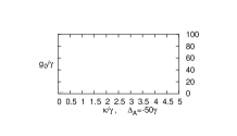
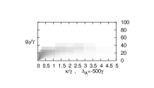
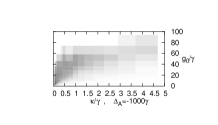
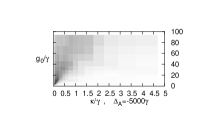
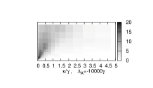
Figure 6: Correlation vs $\kappa$ and $g_{0}$ at various detunings. At small detunings $|\Delta_{A}|<100\gamma$ the atoms are cooled but not trapped, correlation cannot be measured. At higher detunings trapping is good enough, and the correlation strength measured as described in the article is shown in with shades of gray.

At atomic detunings of $100\gamma$ or less, the atoms are cooled but generally not trapped by the cavity, except for a small region of $g_{0}<5\gamma$ and $\kappa<\gamma$. In that case the motion of two atoms will not be correlated. For detunings as large as $5000\gamma$, the cavity field traps and cools the atoms for any considered values of the parameters. The correlation becomes apparent for $g_{0}>40\kappa$, and grows weaker if $g_{0}$ is further increased.

IV.2 Correlation and cooling

A decisive advantage of cavity cooling of an atom is the fact that it needs little spontaneous emission horak97 . It has been argued that this is a single atom effect and correlations established between the atoms’ motion will decrease efficiency or even turn off cooling gangl99 for a trapped thermal ensemble. On the other hand, in some simulations for very weakly bound atoms, this effect seemed not to play any role horak01 .

In our model we can now study the effect of correlations on cavity cooling in a very controlled way for a large range of parameters. We performed several runs of our simulation with different cavity parameters and at different detunings, comparing the equilibrium temperature for one and two atoms in the cavity. Our results are plotted in Figs. 7 (one atom) and 8 (two atoms). All shades of gray show temperatures below Doppler temperature $\hbar\gamma$, while black denotes temperatures above that value.

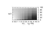
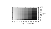
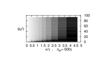
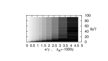
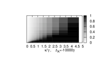
Figure 7: One atom in the cavity: final temperature vs. $\kappa$ and $g_{0}$, for different atomic detunings. Temperature is shown in units of $\hbar\gamma$ with shades of gray. Black denotes temperature above the Doppler limit of $\hbar\gamma$.

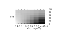
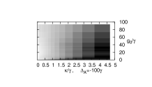
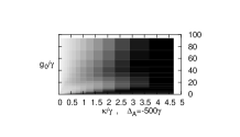
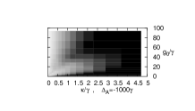
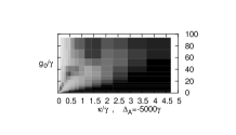
Figure 8: Two atoms in the cavity: final temperature vs. $\kappa$ and $g_{0}$, for different atomic detunings. Temperature is shown in units of $\hbar\gamma$ with shades of gray, as in Figure 7. For low atomic detuning $|\Delta_{A}|<100\gamma$ the temperature is the same as in the one-atom case. For large atomic detuning new structures appear in the plots.

Putting one atom into the cavity (Fig. 7), we find that sub-Doppler cooling is achieved in the good-coupling regime $g_{0}>\kappa,\gamma$. In that regime, the final temperature does not depend on $g_{0}$, but is approximately proportional to $\kappa$, as expected from previous work domokos01a ; domokos02 . Here one has to be cautious of the results, since if the atom’s kinetic energy is only a few times the ground-state energy of the harmonic trap potential, the validity of the semiclassical approximation can be questioned.

Interestingly, the temperature plots look different if we load two atoms into the cavity (Fig. 8). At moderately large detunings, $\Delta_{A}=-50\gamma$ and $\Delta_{A}=-100\gamma$, temperatures are the same as in the single-atom case. In these cases the atoms are cooled, but not trapped, by the cavity field. At larger detunings, $\Delta_{A}=-500\gamma$ and larger, we see regions in the plot where “extra heating” compared to the single-atom case is observed. This effect is most prominent at extremely large detunings $\Delta_{A}=-5000\gamma$ and $\Delta_{A}=-10^{4}\gamma$, where for $\kappa<\gamma$ a new structure appears in the temperature plots. This points to the highly reduced efficiency of cavity cooling: whereas for a single atom a better resonator (lower $\kappa$) implies lower final temperature, if there are two atoms in the cavity, decreasing $\kappa$ can increase the temperature.

Comparison of the temperature plots in Figs. 7 and 8 with the plots of the correlation strength in Fig. 6 reveals strong similarities. Indeed one sees that the excess heating caused by the presence of the other atom coincides with the buildup of correlations in the motion. In other words, the correlation established between two atoms results in a loss of efficiency of cavity cooling, with final temperatures pushed up to the Doppler limit.

IV.3 The origin of correlation: numerical tests

As we have seen above, the motion of the atoms becomes correlated due to the cavity-mediated cross-talk. This interaction occurs via the force, via the friction, and via the diffusion as well. We would like to know which of these interaction channels is responsible for the correlation. In our simulation we can conveniently answer this question if we artificially weaken only particular channels of interaction and measure the correlation.

The interaction can be eliminated from the deterministic force using the approximation (15). Friction and diffusion contain interaction at various levels. On the one hand, cross-friction and cross-diffusion are direct interactions between the atoms. On the other hand – through the determinant $\mathcal{D}^{\prime}$ – the positions of both atoms influence the friction and diffusion constants for the other atoms. This parametric interaction was not analyzed, but does not seem to play a prominent role. Both cross-friction and cross-diffusion can be eliminated by simply suppressing the off-diagonal terms in the friction and diffusion matrices.

The elimination of the interaction can be made continuous with mixing parameters $0\leq y_{F},y_{\beta},y_{\mathcal{D}}\leq 1$, giving the force, the friction, and the diffusion with the following formulae:

$$F^{\prime} =y_{F}F+(1-y_{F})F_{0},$$ (21)

$$\beta_{km}^{\prime} =y_{\beta}\beta_{km}+\delta_{km}(1-y_{\beta})\beta_{km};$$ (22)

$${\mathcal{D}}_{km}^{\prime} =y_{\mathcal{D}}{\mathcal{D}}_{km}+\delta_{km}(1-y_{\mathcal{D}}){\mathcal{D}}_{km}.$$ (23)

We show an example of what this gives for detuning $\Delta_{A}=-5000\gamma$, decay rate $\kappa=0.5\gamma$ and coupling $g_{0}=30\gamma$ in Fig. 9.

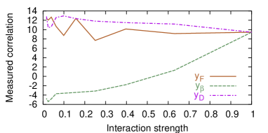
Figure 9: Correlation for various interaction channel strengths. The interaction via the conservative, the friction, and the diffusion forces is weakened by the mixing ratios $y_{F}$, $y_{\beta}$ and $y_{\mathcal{D}}$, as described in the text. The correlation strength was then measured using our correlation parameter. Cross-friction is seen to play the dominant role in the establishment of correlation.

The results of these investigations are quite unanimous. It can be seen that linearization of the potential has no systematic effect on correlation strength, and correlations are slightly enhanced if the noise is decorrelated. If cross-friction is eliminated, however, all correlations disappear. We can therefore conclude that the dominant effect leading to correlated motion is related to cross-friction.

V The origin of correlation: analytical expansion for deep trapping

The emergence of motional correlations between trapped atoms can be examined analytically using the formulas presented in Section III. Both friction and diffusion matrices have an “isotropic” term proportional to $\delta_{km}$, which acts on each atom separately, and an “interaction” term, containing cross-friction and cross-diffusion. The latter can be rewritten in the following form, using the notation $g_{k}=g(\mathbf{x}_{k})$:

$$\frac{2\hbar\eta^{2}}{\left|{\mathcal{D}^{\prime}}\right|^{2}}P(\{\mathbf{x}_{l}\})\begin{pmatrix}\mathbf{\nabla}_{1}g_{1}^{2}\\ \vdots\\ \mathbf{\nabla}_{N}g_{N}^{2}\end{pmatrix}\circ\begin{matrix}\big{(}\mathbf{\nabla}_{1}g_{1}^{2}&\cdots&\mathbf{\nabla}_{N}g_{N}^{2}\big{)}\\ \vphantom{\mathbf{\nabla}_{2}g_{2}^{2}}\\ \vphantom{\mathbf{\nabla}_{2}g_{2}^{2}}\\ \vphantom{\mathbf{\nabla}_{2}g_{2}^{2}}\end{matrix},$$ (24)

where the prefactor $P$ depends on the positions of all atoms symmetrically.

For well-trapped atoms $x_{k}\ll\lambda$ ($x_{k}$ denoting the distance of atom $k$ from the nearest trapping site), the coupling constants can be approximated as

$$g_{k}=g(x_{k})=g_{0}\cos(k_{C}x_{k})\approx g_{0}\left(1-\frac{1}{2}\,k_{C}^{2}x_{k}^{2}\right).$$ (25)

Substituting these into the interaction parts of the matrices (24) yields:

$$\frac{8\hbar\eta^{2}}{\left|{\mathcal{D}^{\prime}}\right|^{2}}P(\{\mathbf{x}_{l}\})g_{0}^{4}k_{C}^{4}r^{2}\begin{pmatrix}x_{1}/r\\ \vdots\\ x_{N}/r\end{pmatrix}\circ\begin{matrix}\big{(}x_{1}/r&\cdots&x_{N}/r\big{)}\\ \vphantom{x_{2})}\\ \vphantom{x_{2})}\end{matrix},$$ (26)

where the “radius”, $r=\left({\sum_{l}x_{l}^{2}}\right)^{\frac{1}{2}}$, is the distance of the system from the origin in the coordinate space. This matrix is a projector to the vector $\left(x_{1},\ldots,x_{N}\right)$, and hence the interaction terms affect only the “radial” motion.

In the well-trapped case we can write the friction and diffusion matrices to second order in the coordinates $x_{l}$ as:

$${\boldsymbol{\beta}}_{km} ={\beta}_{0}\delta_{km}+\beta_{1}x_{k}x_{m},$$ (27)

$${\mathcal{D}}_{km} ={\mathcal{D}}_{0}\delta_{km}+{\mathcal{D}}_{1}x_{k}x_{m}.$$ (28)

The following notation is used:

$${\beta}_{0} =2\hbar\frac{\eta^{2}}{\left|{\mathcal{D}^{\prime}_{0}}\right|^{2}}\gamma g_{0}^{2}k_{C}^{2}\frac{2\Delta_{A}}{\Delta_{A}^{2}+\gamma^{2}}k_{C}^{2}x_{k}^{2},$$ (29)

$${\mathcal{D}}_{0} =2\hbar^{2}\frac{\eta^{2}}{\left|{\mathcal{D}^{\prime}_{0}}\right|^{2}}\gamma g_{0}^{2}k_{C}^{2}\left(\frac{2}{5}+\frac{3}{5}k_{C}^{2}x_{k}^{2}\right),$$ (30)

$${\beta}_{1} =2\hbar\frac{\eta^{2}}{\left|{\mathcal{D}^{\prime}_{0}}\right|^{2}}g_{0}^{4}k_{C}^{4}\Im\left\{\frac{1}{{\mathcal{D}^{\prime}_{0}}^{2}}\biggl{[}\mathcal{D}^{\prime}_{0}(1-3\chi)+\right.$$ (31)

$$\left.\biggl{.}2(1-\chi)\Bigl{(}(i\Delta_{A}-\gamma)^{2}-\sum_{l}g(\mathbf{x}_{l})^{2}\Bigr{)}\biggr{]}\right\},$$ (32)

$${\mathcal{D}}_{1} =2\hbar^{2}\frac{\eta^{2}}{\left|{\mathcal{D}^{\prime}_{0}}\right|^{2}}g_{0}^{4}k_{C}^{4}\,4\frac{\kappa\Delta_{A}+\gamma\Delta_{C}}{\left|{\mathcal{D}^{\prime}_{0}}\right|^{2}},$$ (33)

where $\mathcal{D}^{\prime}_{0}$ stands for the Bloch determinant $\mathcal{D}^{\prime}$ defined in eq. (7), evaluated at the trapping site. Near the trapping site all $x_{k}$ go to zero, and only $\mathcal{D}_{0}$ remains finite. This prevents the atoms from stopping completely: they are “heated out” from the trapping sites themselves. At some distance from the trapping sites the interaction terms become important as well, in the coordinate space this induces extra diffusion and friction in the radial direction. Provided $g_{0}$ is high enough, radial friction is enhanced much more than radial diffusion, leading to a “freezing out” of the radial mode, i.e. a motion at approximately constant distance from the origin.

VI Conclusions

As pointed out in several previous papers, the motion of particles in a cavity is coupled quite generally through the field mode. This implies the buildup of motional correlations, which we have investigated here in more detail. In general we found that in steady state these correlations are hard to see directly and it is difficult to find good qualitative measures to characterize them. Mostly they are strongly perturbed by various diffusion mechanisms. However, they still play an important role in the dynamics and thus can be observed indirectly. As one consequence they can lead to a significant change (increase) in the steady temperature, which directly relates to trapping times and localization properties. This poses limits to cavity induced cooling for large particle numbers.

From the various mechanisms at work, cross-friction turns out to be the most important. It creates correlation and leads to a fast thermalization of two distant particles without direct interaction. Hence, this mechanism should prove vital for the implementation of sympathetic cooling of distant ensembles coupled by a far off-resonant cavity field. In order to get efficient coupling the two species should have comparable oscillation frequencies, so that correlation buildup and thermalization is fast. The finesse of the cavity should also be large (long photon lifetime).

The second important coupling mechanism, which works via the joint steady state potentials, was suggested for use in the implementation of conditional phase shifts hemmerich99 . It can be viewed as a cavity-enhanced dipole–dipole coupling. Although this contribution will become more important for larger atom-field detunings, the conditions for this part to dominate the dissipative cross-friction seem rather hard to achieve in practice. Finally we found that the noise forces acting on different atoms contain nonlocal correlations too. These are particularly important for large detunings and relatively low photon numbers, where spontaneous emission is strongly reduced. As a result they could seriously perturb bipartite quantum gates in cavities.

References

- (1) P. Domokos and H. Ritsch, J. Opt. Soc. Am. B 20, 1098 (2003).
- (2) V. Vuletić, H. W. Chan, and A. T. Black, Phys. Rev. A 64, 033405 (2001).
- (3) S. J. van Enk, J. McKeever, H. J. Kimble, and J. Ye, Phys. Rev. A 64, 013407 (2001).
- (4) P. Münstermann et al., Phys. Rev. Lett. 84, 4068 (2000).
- (5) D. Kruse et al., Phys. Rev. A 67, 051802 (2003).
- (6) A. C. Doherty, A. S. Parkins, S. M. Tan, and D. F. Walls, Phys. Rev. A 56, 833 (1997).
- (7) T. W. Mossberg, M. Lewenstein, and D. J. Gauthier, Phys. Rev. Lett. 67, 1723 (1991).
- (8) P. Maunz et al., Nature 428, 50 (2004).
- (9) A. B. Mundt et al., Phys. Rev. Lett. 89, 103001 (2002).
- (10) G. R. Guthöhrlein et al., Nature 414, 49 (2002).
- (11) A. T. Black, H. W. Chan, and V. Vuletić, Phys. Rev. Lett. 91, 203001 (2003).
- (12) J. A. Sauer et al., quant-ph/0309052 (unpublished).
- (13) D. Kruse, C. von Cube, C. Zimmermann, and P. W. Courteille, Phys. Rev. Lett. 91, 183601 (2003).
- (14) A. Hemmerich, Phys. Rev. A 60, 943 (1999).
- (15) A. Griessner, D. Jaksch, and P. Zoller, submitted to PRA (unpublished).
- (16) J. McKeever et al., Nature 425, 268 (2003).
- (17) A. Kuhn, M. Hennrich, and G. Rempe, Phys. Rev. Lett. 89, 067901 (2002).
- (18) P. Horak and H. Ritsch, Phys. Rev. A 64, 033422 (2001).
- (19) T. Fischer et al., New J. of Phys. 3, 11.1 (2001).
- (20) M. Gangl and H. Ritsch, Phys. Rev. A 61, 043405 (2000).
- (21) R. Bonifacio, G. Robb, and B. M. Neil, Phys. Rev. A 56, 912 (1997).
- (22) D. Jaksch et al., Phys. Rev. Lett. 86, 4773 (2001).
- (23) M. Gangl and H. Ritsch, Phys. Rev. A 61, 011402 (1999).
- (24) P. Domokos and H. Ritsch, Phys. Rev. Lett. 89, 253003 (2002).
- (25) H. W. Chan, A. T. Black, and V. Vuletić, Phys. Rev. Lett. 90, 063003 (2003).
- (26) P. Domokos, T. Salzburger, and H. Ritsch, Phys. Rev. A 66, 043406 (2002).
- (27) T. Fischer et al., Phys. Rev. Lett. 88, 163002 (2002).
- (28) P. Horak et al., Phys. Rev. Lett. 79, 4974 (1997).
- (29) P. Domokos, P. Horak, and H. Ritsch, Journal of Physics B: At. Mol. Opt. Phys. 34, 187 (2001).