Dynamical parameter estimation using realistic photodetection

Abstract

We investigate the effect of imperfections in realistic detectors upon the problem of quantum state and parameter estimation by continuous monitoring of an open quantum system. Specifically, we have reexamined the system of a two-level atom with an unknown Rabi frequency introduced by Gambetta and Wiseman [Phys. Rev. A 64, 042105 (2001)]. We consider only direct photodetection and use the realistic quantum trajectory theory reported by Warszawski, Wiseman, and Mabuchi [Phys. Rev. A 65, 023802 (2002)]. The most significant effect comes from a finite bandwidth, corresponding to an uncertainty in the response time of the photodiode. Unless the bandwidth is significantly greater than the Rabi frequency, the observer’s ability to obtain information about the unknown Rabi frequency, and about the state of the atom, is severely compromised. This result has implications for quantum control in the presence of unknown parameters for realistic detectors, and even for ideal detectors, as it implies that most of the information in the measurement record is contained in the precise timing of the detections.

I Introduction

Quantum parameter estimation originated with the work by Helevo Hol82 and Helstrom Hel76 and is usually formulated as follows. A known quantum state undergoes some evolution. This evolution is usually unitary but need not be ChuNie97 , and is parameterized by one or more unknown parameters. The goal is to estimate these parameters by making a measurement on the final state. In a recent paper, two of us Jay , following Mabuchi MabuchiEst , considered the situation in which an open quantum system parameterized by an unknown dynamical parameter is estimated through continuous-in-time measurements of the environment. Ref. Jay also focussed on the conditioned state and how the lack of information about the parameter affects its purity. These two papers are part of a small but growing body of work including DohertyStateDeterm and DohertyOptQPE (and references therein) that address the problem of reducing classical uncertainties in the evolution of quantum systems by performing continuous-in-time measurements.

In Ref. Jay , the system is taken to be a damped, classically driven two-level atom (TLA) with a driving Hamiltonian ($\propto\hat{\sigma}_{x}$ in a rotating frame) with an uncertain driving strength $\Omega$. The physical scenario the authors give for this is as follows. An atom is placed in a classical standing wave, thus experiencing a Rabi frequency of

$$\Omega=\Omega_{{\rm max}}\sin(kx),$$ (1)

where $k$ is the wavevector for the classical field and $x$ is the position of centre of mass of the atom. Gambetta and Wiseman then assume that the TLA is equally likely to be placed at any position in the standing wave. Hence, a range of $-\Omega_{{\rm max}}\leq\Omega\leq\Omega_{{\rm max}}$ exists for the possible driving strength. It is also assumed that the TLA has zero translational motion. This can be justified by assuming that the TLA is fixed by a radio frequency Paul trap or similar confining mechanism MabuchiEst . Although it is shown that continual efficient measurement upon the output electromagnetic field of a TLA leads to information gain about the driving strength, the amount of information gained depends strongly on the measurement scheme used. The purity of the conditional state also depends strongly on the measurement scheme, but the performance of schemes by these different criteria are not well correlated at all Jay .

In this paper, we consider only one sort of detection: direct detection, but we consider imperfect detection. This allows us to address the following two questions. First, what (qualitatively) are the aspects of the ideal measurement record that contain the information about the system state and the unknown parameter? Second, in practice, how badly would the amount of information gained be affected by detectors with realistic imperfections. To treat realistic detection we use the theory developed in Refs. WarWisMab02 ; WarWis03a ; WarWis03b . This generalized the theory of quantum trajectories Car93b ; BelSta92 ; Bar93 ; DalCasMol92 ; GarParZol92 ; Wis96a by determining the state of the system conditioned upon the output of a detector that has dead-time ($\tau_{\rm dd}$), dark counts at rate $\gamma_{\rm dk}$, inefficiency $\eta$, and finite bandwidth $\gamma_{\rm r}$. A diagram of this detector is displayed in Fig. 1.

Figure 1: A schematic illustrating realistic direct detection. The atom is placed at the focus of a parabolic mirror such that all the fluorescence enters the realistic detector. Realistic photon counting is performed by an avalanche photodiode. The quantum efficiency $\eta$ of the diode is represented by the the beam-splitter (BS). Single arrowheads within the realistic photodetector indicate Poisson processes. The microscopic detector states are indicated by a 0, 1, and 2.

The reciprocal of the bandwidth $\gamma_{\rm r}^{-1}$ sets the scale for the uncertainty in the delay between the absorption of photon (which is synonymous with its detection in an ideal detector) and the avalanche of charge which registers this at a macroscopic level in a realistic detector. We find that a finite bandwidth has the greatest effect on our parameter estimation problem. This tells us that it is the timing between detections, not the steady state detection rate, that contains the majority of the information gained. Unless the bandwidth of the detector is substantially greater than $\Omega_{\rm max}$, the rate of gain of information about $\Omega$ is much reduced, and consequently the purity of the system is also. Like the work of Ref. Jay this has important implications for the robustness of quantum feedback control (see for example Refs. Dohe2000 ; WisManWan02 ).

This paper is structured as follows. In Sec. II we begin with some numerical results to motivate the theoretical developments in the remainder of the paper. In Sec. III we briefly review the theory of parameter estimation based on linear quantum trajectories in Ref. Jay , and show how it can be applied to realistic detection. In Sec. IV we use this theory to investigate the evolution of the conditional state for an initially unknown parameter, and in Sec. V we investigate the rate of information gain about the parameter. We conclude with a discussion in Sec. VI.

II Conditional Probability Distribution for Driving Strength

Before providing a theoretical basis, some numerical results are provided to give the reader an insight into the effects of realistic detection on parameter estimation. With an example in mind, the theory contained in the following section should also prove to be more transparent.

We begin by looking at how an observer’s probability distribution for the driving strength evolves given a single measurement record (trajectory). Details of the numerical techniques employed to do this will be given at the end of the next section. The distribution is denoted by $P(\Omega|{\bf I}_{[0,t)})$, where ${\bf I}_{[0,t)}$ represents the measurement record. Obviously, ${\bf I}_{[0,t)}$ refers to different events for ideal and realistic detection: it is a record of the times of photodetections and of avalanches, respectively. The initial distribution can be found from Eq. (1) with $x$ taken to have a flat distribution. The result is

$$P_{0}(\Omega)=\frac{1}{\pi\sqrt{\Omega_{{\rm max}}^{2}-\Omega^{2}}}.$$ (2)

The unconditioned evolution of the atom (which is independent of the scheme, or quality, of detection) is given by the master equation (ME)

$$\dot{\rho}(t)=-\frac{i\Omega}{2}[\hat{\sigma}_{x},\rho(t)]+\Gamma{\cal D}[\hat{\sigma}]\rho(t)={\cal L}_{\Omega}\rho(t).$$ (3)

Here $\Omega$ is assumed known, $\Gamma$ is the spontaneous emission rate (which we will set equal to unity), $\hat{\sigma}$ is the atomic lowering operator, and $\hat{\sigma}_{x}=\hat{\sigma}+\hat{\sigma}^{\dagger}$. The superoperator ${\cal D}$ gives the damping of the system into the environment and is defined as WisMil93c

$${\cal D}[\hat{a}]\rho=\hat{a}\rho\hat{a}^{\dagger}-\mbox{$\frac{1}{2}$}\left\{{\hat{a}^{\dagger}\hat{a}\rho+\rho\hat{a}^{\dagger}\hat{a}}\right\}.$$ (4)

A comparison of ideal and realistic detection is given in Fig. 2. In this figure $\Omega_{\rm true}=4\Gamma$, but the observer does not know this, but rather has knowledge described by the prior distribution (2) with $\Omega_{\rm max}=10\Gamma$. As time goes on, the detection record reveals more about $\Omega_{\rm true}$, and this probability is updated in a Bayesian manner. Note that for both ideal and realistic detectors, the distribution always remains symmetric. This is because the sign of $\Omega$ cannot be determined from direct detection. Photoemissions depend only upon the mean of $\hat{\sigma}_{z}$, and that is independent of whether the TLA state rotates clockwise or counterclockwise around the $\hat{\sigma}_{x}$ axis.

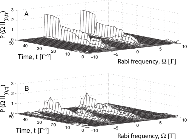
Figure 2: Plots (A) and (B) show how the probability distribution for $\Omega$ typically evolves while continuous direct detection is performed on the output of the quantum system (a TLA inside an optical cavity). Plot (A) is for ideal detection, while (B) is for realistic detection. The parameters used for the photon counter were $\eta=100\%$, and $\gamma_{{\rm r}}=7\Gamma$, $\tau_{{\rm dd}}=0$, $\gamma_{{\rm dk}}=0$. The value of $\Omega$ used to generate ${\bf I}_{[0,t)}$ was $\Omega_{{\rm true}}=4\Gamma$. The maximum allowed value for $\Omega$ is $\Omega_{{\rm max}}=10\Gamma$.

In Fig. 2, we have chosen a realistic detector whose only imperfection is a finite bandwidth equal to 7$\Gamma$ (see figure caption). It can be seen that the degradation of the quality of measurement is quite large even though our ‘realistic’ detector is well beyond current technology. If we choose the realistic parameters for an APD (avalanche photodioide) used in Refs. WarWisMab02 ; WarWis03b we obtain results that are so far from those of ideal detection that a comparison lacks interest.

The fact that the chosen detector parameters give results that are still poor compared to ideal measurement is a little surprising. Very few photodetections are missed under realistic detection with a finite $\gamma_{{\rm r}}$ being the only imperfection. It illustrates that the rate of information gain is very sensitive to an uncertainty in the state of the TLA after a jump.

The plot for realistic detection, Fig. 2 (B), also shows that it is difficult to distinguish between $\Omega_{{\rm true}}$ and an integer multiple of $\Omega_{{\rm true}}$, say $m\Omega_{{\rm true}}$ (for this figure this occurs only for $|\Omega_{{\rm true}}|$ and $2|\Omega_{{\rm true}}|$). By $\Omega_{{\rm true}}$ we mean the actual driving strength that exists, but which is initially unknown to the observer. This difficulty exists because the evolution for these two proposed values of the driving strength will place the TLA in the excited state at the same time every integer oscillation (at the smaller frequency). Hence, for certain times there will be a strong correlation between the probabilities of decay. Obviously, a photoemission can still occur when a driving strength of $2|\Omega_{{\rm true}}|$ would place the TLA very near ground state, thus ruling out that possible value. Whether these decays that are discriminatory in this sense are detected or not depends on the choice (and duration) of the quantum trajectory in question. In Fig. 2 (B) a small but, persistent (at least up to $t=50$) probability for $|\Omega|=2|\Omega_{{\rm true}}|$ exists.

It is worth mentioning that the plots in Fig. 2 are based on the ‘same’ photo-absorptions in the ideal and realistic cases. This is possible using the simulation technique of Refs. WarWis03b , in which the realistic quantum trajectory can be assured to be consistent with the ideal quantum trajectory.

III Parameter and State Estimation Theory

We now briefly present the theory of parameter and state estimation in the context that is relevant to this paper. The specific problem that we wish to address involves calculating the new probability distribution for $\Omega$ and also obtaining the best estimate of the TLA state, based on the measurement record. Bayesian statistics are required, with the new distribution, based on ${\bf I}_{[0,t)}$, given by BayesBook

$$P(\Omega|{\bf I}_{[0,t)})=\frac{P({\bf I}_{[0,t)}|\Omega)P_{0}(\Omega)}{\int P({\bf I}_{[0,t)}|\Omega)P_{0}(\Omega)d\Omega}.$$ (5)

The best estimate of the TLA state is found from Jay

$$\rho_{{\bf I}}(t)=\frac{\int\tilde{\rho}_{{\bf I},\Omega}(t)P_{0}(\Omega)d\Omega}{\int P({\bf I}_{[0,t)}|\Omega)P_{0}(\Omega)d\Omega},$$ (6)

where $\tilde{\rho}_{{\bf I},\Omega}(t)$ is the unnormalised state of the TLA given that there was a measurement record ${\bf I}_{[0,t)}$ and that the driving strength was $\Omega$.

In this paper we leave the state unnormalised even after jumps, so that

$$\rho_{{\bf I},\Omega}(t)=\frac{\tilde{\rho}_{{\bf I},\Omega}(t)}{P({\bf I}_{[0,t)}|\Omega)}$$ (7)

meaning that $P({\bf I}_{[0,t)}|\Omega)$ is actually equal to the norm of the TLA state, when it is evolved with $\Omega$ under ${\bf I}_{[0,t)}$. Ideally ${\bf I}_{[0,t)}$ would be an experimental record, but for convenience we simulate it using $\Omega_{{\rm true}}$ and then ‘forgetting’ it. The integrals in Eqs. (5)–(6) require the simulation of the evolution for the entire range of $\Omega$. This means that the process is very time consuming as many trajectories (for the different $\Omega$’s) have to be run in order to obtain a single trajectory for $P(\Omega|{\bf I}_{[0,t)})$ or $\rho_{{\bf I}}(t)$.

In order to treat realistic detection, it is necessary to describe not just the state of the TLA, but also the state of a detector (treated classically) which is correlated with the atomic state WarWisMab02 ; WarWis03a . We do this by introducing a set of three operators $\rho_{{\bf I},s}(t)$ for this supersystem, where here $s=0,1,2$ represents the three classical detector states. These correspond to the ready state ($s=0$), the avalanching state ($s=1$) and the resetting state ($s=2$). Refer to Fig. 1 for details. The state of the TLA is defined as $\rho_{\bf I}(t)=\rho_{{\bf I},0}(t)+\rho_{{\bf I},1}(t)+\rho_{{\bf I},2}(t)$. Equation (6) is trivially generalized to give the best estimate of the supersystem state $\rho_{{\bf I},s}(t)$:

$$\rho_{{\bf I},s}(t)=\frac{\int\tilde{\rho}_{{\bf I},\Omega,s}(t)P_{0}(\Omega)d\Omega}{\int P({\bf I}_{[0,t)}|\Omega)P_{0}(\Omega)d\Omega}.$$ (8)

The three equations, Eqs. (5)–(6) and Eq. (8), are unusable in their present form as $P({\bf I}_{[0,t)}|\Omega)$ and the norm of $\tilde{\rho}_{{\bf I},\Omega}(t)$ (which is equal to $P({\bf I}_{[0,t)}|\Omega)$) will become extremely small as $t$ increases. This will be true even for $\Omega=\Omega_{{\rm true}}$, as can be seen by considering the probability of a string of measurement results occurring. The probability of a jump in a given infinitesimal interval is never greater than $\Gamma dt$, so that the norm of the state after $m$ jumps would be less than $(\Gamma dt)^{m}$ (since the no-jump evolution also decreases the norm of the state). In simulations, a time step of $dt=10^{-4}\Gamma^{-1}$ is typical. Thus, numerical error introduced by computer round-off necessitates a different approach which we now explain.

III.1 Linear Quantum Trajectories

In linear quantum trajectories Wis96a , the state is multiplied by a predetermined factor after every measurement event. The normalisation constants are chosen so that the norm of the states corresponding to the most likely values of $\Omega$ stay relatively close to unity. Each possible measurement result, $r$, has an ‘ostensible’ Wis96a probability, $\Lambda(r)$ associated with it, that we use as the normalising factor. Therefore, we have

$$\bar{\rho}_{{\bf I},\Omega,s}(t)=\frac{\tilde{\rho}_{{\bf I},\Omega,s}(t)}{\Lambda({\bf I}_{[0,t)})},$$ (9)

where $\bar{\rho}_{{\bf I},\Omega,s}$ is the supersystem state when linear quantum trajectories are used and $\Lambda({\bf I}_{[0,t)})$ is the ostensible probability for getting ${\bf I}_{[0,t)}$,

$$\Lambda({\bf I}_{[0,t)})=\Lambda(r_{k})\Lambda(r_{k-1})\ldots\Lambda(r_{1}).$$ (10)

Here, we have assumed that the time interval $[0,t)$ has been divided into a very large number, $k=t/dt$, of discrete measurement times. The actual probability of getting ${\bf I}_{[0,t)}$, given $\Omega$ is

$$P({\bf I}_{[0,t)}|\Omega)=\Lambda({\bf I}_{[0,t)})\sum_{s}{\rm Tr}[\bar{\rho}_{{\bf I},\Omega,s}(t)],$$ (11)

where the trace is over the TLA and the summation is over the detector states.

This allows Eq. (5) and Eq. (8) to be written as Jay

$$P(\Omega|{\bf I}_{[0,t)})=\frac{\sum_{s}{\rm Tr}[\bar{\rho}_{{\bf I},\Omega,s}(t)]P_{0}(\Omega)}{\int\sum_{s}{\rm Tr}[\bar{\rho}_{{\bf I},\Omega,s}(t)]P_{0}(\Omega)d\Omega}$$ (12)

and

$$\rho_{{\bf I},s}(t)=\frac{\int\bar{\rho}_{{\bf I},\Omega,s}(t)P_{0}(\Omega)d\Omega}{\int\sum_{s}{\rm Tr}[\bar{\rho}_{{\bf I},\Omega,s}(t)]P_{0}(\Omega)d\Omega}.$$ (13)

Since ${\rm Tr}[\bar{\rho}_{{\bf I},\Omega,s}(t)]$ is of order unity for the most likely $\Omega$’s the problems associated with using ${\rm Tr}[\tilde{\rho}_{{\bf I},\Omega,s}(t)]$ have been avoided. The best estimate of the system state allows the conditional evolution of a single stochastic record to be investigated, while $P(\Omega|{\bf I}_{[0,t)})$ will allow calculation of the information gain (see following).

In this paper, we choose the ostensible probabilities to be

$$\Lambda(1)=\epsilon dt,$$ (14)

where $r=1$ indicates the detection of a photon (ideal detector) or an avalanche (realistic detector). No detection ($r=0$) has an ostensible probability $\Lambda(0)=1-\epsilon dt$. With these ostensible probabilities, the linear quantum trajectory equations for the supersystem describing realistic detection WarWisMab02 ; WarWis03a become

$$d\bar{\rho}_{0}(t) = dt\left({\cal L}_{\Omega}-\gamma_{{\rm dk}}-\eta\Gamma{\cal J}[\hat{\sigma}]+\epsilon\right)\bar{\rho}_{0}(t)$$ (15)

$${-}\,d{\cal N}(t)\bar{\rho}_{0}(t){+}d{\cal N}(t)(t-\tau_{{\rm dd}})\bar{\rho}_{2}(t)$$

$$d\bar{\rho}_{1}(t) = dt\left({\cal L}_{\Omega}-\gamma_{{\rm r}}+\epsilon\right)\bar{\rho}_{1}(t)+dt\left(\eta\Gamma{\cal J}[\hat{\sigma}]+\gamma_{{\rm dk}}\right)$$ (16)

$${\times}\,\bar{\rho}_{0}(t){-}d{\cal N}(t)\bar{\rho}_{1}$$

$$d\bar{\rho}_{2}(t) = dt\left({\cal L}_{\Omega}+\epsilon\right)\bar{\rho}_{2}(t)+{d{\cal N}(t)}\bar{\rho}_{1}(t)/{\epsilon}$$ (17)

$${-}\,d{\cal N}(t)(t-\tau_{{\rm dd}})\bar{\rho}_{2}(t).$$

Here $d{\cal N}(t)=0,1$, the increment in the number of avalanches, is equivalent to the measurement result $r$ in the time interval $[t,t+dt)$. We maintain the symbol ${\bf I}_{[0,t)}$ for the record of avalanches in the interval $[0,t)$, but for clarity we have omitted the subscripts ${\bf I}$ and $\Omega$ for the $\rho(t)$’s. The superoperator ${\cal J}$ is defined by WisMil93c

$${\cal J}[\hat{a}]\rho\equiv\hat{a}\rho\hat{a}^{\dagger}.$$ (18)

For simulation purposes we take

$$\epsilon=\eta\frac{\Gamma\Omega_{\rm true}^{2}}{2\Omega_{\rm true}^{2}+\Gamma^{2}},$$ (19)

the expected detection rate in steady state (ignoring any dead time) when $\Omega$ is known. This is allowed as the results of the simulation are independent of $\epsilon$, thus we are free to choose any value. Note that renormalisation of $\rho(t)$ is occurring even when the detector is resetting and the probability of an avalanche is strictly zero. This illustrates the flexibility of the ostensible probabilities, where the only concern is maintaining a norm of order unity.

IV Conditional State Evolution

Now that we have explained how the numerical results of Sec. II were obtained, we return to these simulations to investigate the conditional state evolution in a typical realistic quantum trajectory. In Fig. 3 we see how $z(t)$ (the mean of $\hat{\sigma}_{z}$) behaves under a variety of circumstances. Specifically, we consider known $|\Omega_{{\rm true}}|$ and ideal detection (thin dashed line), unknown $|\Omega_{{\rm true}}|$ (that is, an initial distribution given by Eq. (2)) and ideal detection (thin solid line), known $|\Omega_{{\rm true}}|$ and realistic detection (thick dashed line) and, finally, unknown $|\Omega_{{\rm true}}|$ and realistic detection (thick solid line). The reason why a comparison is made between the trajectories for a TLA randomly placed in the standing wave of the field and trajectories of known $|\Omega_{{\rm true}}|$, but unknown sign, is that at $t=\infty$ the sign of $\Omega_{{\rm true}}$ will still not be known, as discussed in Sec. II. This allows us to reveal how far the initially unknown $|\Omega_{{\rm true}}|$ trajectories are from their optimal form, given the constraints of direct detection.

Figure 3: Two segments of evolution of $z(t)$ in a typical trajectory are shown. The legend is as follows: thin-lines are for ideal detection, thick-lines are for realistic detection, dashed is for known $|\Omega_{{\rm true}}|$ and solid is for unknown $|\Omega_{{\rm true}}|$. Thus, to be explicit, the thin dashed line is for $|\Omega_{{\rm true}}|$ known and ideal detection, the thin solid line is for $|\Omega_{{\rm true}}|$ unknown and ideal detection, the thick dashed line is for $|\Omega_{{\rm true}}|$ known and realistic detection and, finally, the thick solid line is for $|\Omega_{{\rm true}}|$ unknown and realistic detection. The detector and system parameters (and time units) are as for Fig. 2.

The conditioned state corresponding to a known $|\Omega_{{\rm true}}|$ is formed from

$$\rho_{{\rm I}}(t)=(\rho_{{\rm I},{\Omega_{{\rm true}}}}(t)+\rho_{{\rm I},{-\Omega_{{\rm true}}}}(t))/2.$$ (20)

That is, it is an equal mixture of the two conditioned states obtained with a driving strength of $+\Omega_{{\rm true}}$ and $-\Omega_{{\rm true}}$. Given that we take the TLA as starting in the ground state, these two conditioned states will have the same $z(t)$, but opposite sign for $y(t)$ resulting in $y(t)=0$ for the mixture as initially $P_{0}(\Omega)$ is an even mix of positive and negative $\Omega$. If the initial state of the TLA (which is presumed to be known) gives a finite value for $y(t=0)$ then the time of the first jump will give a very small amount of information about $\Omega_{{\rm true}}$. This is because an early jump would tend to support the conclusion that the TLA had been rotated on the Bloch sphere in the direction that takes it towards the excited state first, while a later jump suggests that the TLA was rotated in the opposite direction. However, the initial state is taken to be the ground state in our simulations. Since for direction detection with no detuning $x(t)=0$ Car93b ; WisMil93c , we have

$$\rho_{{\rm I}}(t)=(I+z(t)\hat{\sigma}_{z})/2,$$ (21)

where $z(t)$ could be obtained from either the $+\Omega_{{\rm true}}$ or $-\Omega_{{\rm true}}$ trajectory. It should now be clear why only $z(t)$ is plotted. In fact, the purity can also be inferred from the $z(t)$ plot as $p_{\rm I}(t)=(1+z^{2}(t))/2$.

As for Fig. 2, the realistic trajectory is forced to be consistent with the ideal trajectory. This is evidenced by the jump times being correlated. Because of the detail of these plots we show two portions of the evolution only, illustrating how improved knowledge over time of the dynamical parameter, $\Omega$, allows closer adhesion to the maximum knowledge trajectory (thin dashed line for ideal detection and thick dashed line for realistic detection).

In the first $10\Gamma^{-1}$ units of time the frequency of oscillation of $z(t)$ for the realistic detection state (solid black line) is poorly defined. One can also see that the frequency is faster than the true frequency, due to $P_{0}(\Omega)$ being peaked at $\pm\Omega_{{\rm max}}$ Jay . The small amplitude of oscillation is also due to the lack of knowledge about $\Omega$. The range of possible frequencies ensures that when one value of $\Omega$ would place the TLA in the excited state, another would place it near the ground state, thus averaging the amplitude of oscillation of $z(t)$ to below unity.

For ideal detection (thin solid line), the frequency of oscillation is also shifting about, but the amplitude of the oscillations have already noticeably increased in size by $t=10\Gamma^{-1}$. Another feature is that jumps take $z(t)$ to $-1$ (a pure state) for ideal detection even if $|\Omega_{{\rm true}}|$ is not known. This is because there is no time delay in conveying the decay of the TLA to the observer. This is not true for realistic detection where the jump is slightly delayed and the TLA will have rotated out of the ground state by some unknown amount.

After $40\Gamma^{-1}$ time units, the ideal detection observer has gained enough information about $|\Omega_{{\rm true}}|$ that $z(t)$ matches well with the ‘ideal’ $z(t)$ (Fig. 3 (B)). The realistic observer’s $z(t)$ is much closer to the ideal than at the start of the trajectory, but some uncertainty still obviously exists.

V Information Gain

We now move away from conditional dynamics and look at how the ensemble averaged gain of information concerning $\Omega$ is affected by realistic detection. As in Jay , the measure used to quantify the quality of information gained about $\Omega$ is $\Delta I_{{\bf I}}$. It is given, in bits, by

$$\Delta I_{{\bf I}} = \int d\Omega P(\Omega|{\bf I}_{[0,t)})\log_{2}P(\Omega|{\bf I}_{[0,t)})$$ (22)

$${-}\,\int d\Omega P_{0}(\Omega)\log_{2}P_{0}(\Omega).$$

As the distribution for $\Omega$ becomes more sharply peaked around $|\Omega_{{\rm true}}|$, $\Delta I_{{\bf I}}$ will increase. Due to the stochastic nature of ${\bf I}_{[0,t)}$, an ensemble of trajectories are run in order to obtain the average, $\Delta I$, of $\Delta I_{{\bf I}}$ that is characteristic of the measurement scheme. Each member of the ensemble is formed by picking an $\Omega_{{\rm true}}$ randomly (but according to the distribution Eq. (2)) and simulating the evolution based on a stochastic trajectory corresponding to that $\Omega_{{\rm true}}$. A single trajectory for each member of an ensemble of $\Omega_{{\rm true}}$’s is sufficient as the averaging of the stochasticity is done over the multitude of $\Omega_{{\rm true}}$’s.

A major difference between parameter estimation for ideal direct detection and realistic direct detection is found when $\Omega_{{\rm true}}\gg\Gamma$. We investigate this regime by varying the value of $\Omega_{{\rm max}}$ used in the simulations. This works as the most likely values for $\Omega_{{\rm true}}$ come from close to $\Omega_{{\rm max}}$. By increasing $\Omega_{{\rm max}}$ we are effectively increasing the values of $\Omega_{{\rm true}}$ used. This method corresponds physically to the TLA being placed randomly in standing waves of different amplitude.

In Fig. 4 (A) the information gain, $\Delta I$, averaged over an ensemble size of $1000$ (that is, $1000$ different $\Omega_{{\rm true}}$’s), is shown for ideal detection. The three plots are for $\Omega_{{\rm max}}=5\Gamma,10\Gamma,20\Gamma$. In Fig. 4 (B) the results are shown for the same values of $\Omega_{{\rm max}}$ when the monitoring is done with realistic detection. Error bars are included as the ensemble size in this case is only $100$, due to the greater computational intensity. As $\Omega_{{\rm max}}$ doubles, the information gain curves for ideal detection are separated by approximately $1$ bit at large $t$. This does not indicate that the detection scheme is more effective at large $\Omega_{{\rm max}}$, rather, it is an artifact of the initial information content of the distribution $P_{0}(\Omega)$. This can easily be shown analytically. Consider the integral

$$\int^{\Omega_{{\rm max}}}_{-\Omega_{{\rm max}}}d\Omega\frac{1}{\pi\sqrt{\Omega_{{\rm max}}^{2}-\Omega^{2}}}\log_{2}\frac{1}{\pi\sqrt{\Omega_{{\rm max}}^{2}-\Omega^{2}}}.$$ (23)

If the change $\Omega^{\prime}_{{\rm max}}\rightarrow m\Omega_{{\rm max}}$ is made, a change of integration variable to $\Omega^{\prime}=m\Omega$ allows the information of the new distribution to be expressed in terms of the old one. The result is

$$\Delta I_{{\bf I},(m\Omega_{{\rm max}})}=\Delta I_{{\bf I},(\Omega_{{\rm max}})}-\log_{2}m.$$ (24)

Thus, every time $\Omega_{{\rm max}}$ is doubled, the initial information decreases by $1$ bit. Since the initial information is being subtracted from the information at time $t$, we can conclude that the width of the $P(\Omega)$ distributions, for different $\Omega_{{\rm max}}$, in the long time limit are roughly equal for ideal detection.

Figure 4: In plot (A) the ensemble averaged information gain for ideal detection is shown for three different values of $\Omega_{{\rm max}}$. In plot (B) the ensemble averaged (over $100$ trajectories) information gain for ideal detection is shown for the same values of $\Omega_{{\rm max}}$. In plot (C) the difference between ideal and realistic detection is shown.

This is qualitatively different from the case of realistic detection where the information gain for $\Omega_{{\rm max}}=5\Gamma$ and $10\Gamma$ are roughly the same and $\Omega_{{\rm max}}=20\Gamma$ sees a significant decrease. Taking into account the fact that as $\Omega_{{\rm max}}$ increases less information is being subtracted away from the information at time $t$, it is clear that realistic detection is becoming considerably worse at distinguishing between candidates for $\Omega_{{\rm true}}$. This is more clearly illustrated in Fig. 4 (C) which shows the difference between ideal and realistic detection information gain for the three values of $\Omega_{{\rm max}}$. We now try to understand these trends by discussing what features of a measurement record allow the information to be accrued.

The most simple (and naive) way to determine the actual driving strength is to analyse the mean steady-state photon counting rate $\langle{\bf I}\rangle_{\rm ss}$. For ideal direct detection this is

$$\langle{\bf I}\rangle_{\rm ss}=\frac{\Gamma\Omega^{2}}{2\Omega^{2}+\Gamma^{2}}.$$ (25)

By using Eq. (25) the mean flux can be matched with a particular $\Omega$, given that $\Gamma$ is known. However, the flux asymptotes to $\Gamma/2$ at large $\Omega$, essentially making one value of $\Omega$ indistinguishable from another. Because ideal detection still gives information at large $\Omega_{{\rm max}}$ we deduce that the specific times at which detections are occurring also play a role in determining $\Omega_{{\rm true}}$.

To consider this effect in more detail we look at the waiting time distribution for photon detections. In perfect direct detection wtime

$$w(\tau)=\frac{\Omega^{2}}{\Omega^{2}-(\Gamma/2)^{2}}e^{-\Gamma\tau/2}\sin^{2}\{\mbox{$\frac{1}{2}$}[\Omega^{2}-(\Gamma/2)^{2}]^{1/2}\tau\},$$ (26)

where $w(\tau)$ is the probability density of a photon being emitted by the TLA at a time $\tau$ after the previous emission. The waiting time, $w(\tau)$, is zero at $\tau=0$ as the TLA in the ground state after a detection. A plot of this function for $\Omega=5\Gamma$, with $\Gamma=1$ is given in Fig. 5 (A). The point that is meant to be taken from this graph is that there are oscillations that make certain emission times more likely (when the TLA is in the excited state) and other times prohibited (when it is in the ground state), given a certain driving strength. These oscillations, which take $w(\tau)$ to zero, are present for all $\Omega>\Gamma/2$, which includes the regime of interest here. This allows the narrowing of the distribution for $\Omega$, based on a measurement record, despite the fact that very little information can be obtained from the mean flux rate.

The waiting time distribution for realistic detection is much more complex. In this case, $\tau$ would be the waiting time between avalanches of the photodiode, rather than emissions of the TLA. One of the difficulties lies in the fact that there is not a definite state of the atom after an avalanche, due to the finite response time. Thus, initial conditions for the TLA must be chosen as being characteristic of the post-avalanche state. We chose them to be the solution to the ME (3) averaged over the time for the avalanche to mature. That is,

$$\rho_{{\rm aval.}}=\gamma_{{\rm r}}\int_{0}^{\infty}e^{-\gamma_{{\rm r}}t}\rho(t)dt,$$ (27)

where $\rho(t)$ is the solution to the ME given that at $t=0$ the TLA is in the ground state. Of course, this will only be true if the dark counts are ignored, which we will do. The integral in Eq. (27) can be carried out analytically with $x=0$ and the $y$ and $z$ components of the state being

$$y_{{\rm aval.}} = \frac{2\Omega(1+\gamma_{{\rm r}})}{(1+3\gamma_{{\rm r}}+2\gamma_{{\rm r}}^{2}+2\Omega^{2})},$$ (28)

$$z_{{\rm aval.}} = -\frac{(2\gamma_{{\rm r}}+1)(1+\gamma_{{\rm r}})}{(1+3\gamma_{{\rm r}}+2\gamma_{{\rm r}}^{2}+2\Omega^{2})},$$ (29)

where we have set $\Gamma=1$.

If we take the simplest case where $\tau_{dd}=0$ and $\gamma_{dk}=0$, then we can use these as the initial conditions for the ready state of the detector. (The case where $\tau_{dd}\neq 0$ is only a little more complicated, because the solutions in Eqs. (28)–(29) can be evolved forward a time $\tau_{{\rm dd}}$ with the ME to give the state of the TLA when the detector becomes ready to detect photons once more.) A series of $6$ linear coupled differential equations must be solved in order to determine $\gamma_{{\rm r}}{\rm Tr}[\tilde{\rho}_{1}(\tau)]=w(\tau)_{{\rm aval.}}$, which is equal to the probability of an avalanche at time $\tau$ (the waiting time). Here, $\tilde{\rho}_{1}(\tau)$ is the solution to the unnormalised evolution equations given in Eqs. (15) and (16) with $\epsilon=0$ and $d{\cal N}\equiv 0$ (no avalanches) from $\tau_{\rm dd}$ to $\tau$.

The $6$ real variables that are necessary can be expressed as a vector $\vec{r}=(\tilde{y}_{0},\tilde{z}_{0},\tilde{P}_{0},\tilde{y}_{1},\tilde{z}_{1},and\tilde{P}_{1})^{\rm T}$, where the the subscripts refer to the detector state and the $P$’s are the probability of occupation. The equations of motion for this vector is $d\vec{r}/dt={\bf A}{\vec{r}}$ where ${\bf A}$ is the following matrix

$$\left(\begin{array}[]{cccccc}-\mbox{$\frac{1}{2}$}&0&-\Omega&0&0&0\\ 0&-\mbox{$\frac{1}{2}$}-\gamma_{{\rm r}}&0&-\Omega&0&0\\ \Omega&0&-1+\frac{\eta}{2}&0&-1+\frac{\eta}{2}&0\\ 0&\Omega&-\frac{\eta}{2}&-1-\gamma_{{\rm r}}&-\frac{\eta}{2}&-1\\ 0&0&-\frac{\eta}{2}&0&-\frac{\eta}{2}&0\\ 0&0&\frac{\eta}{2}&0&\frac{\eta}{2}&-\gamma_{{\rm r}}\end{array}\right),$$ (30)

whereas before we are assuming $\gamma_{{\rm dk}}=0$ and $\Gamma=1$. The variable of interest is then $w(\tau)_{\rm aval}=\gamma_{{\rm r}}\tilde{P}_{1}(\tau)$

Figure 5: In plot (A) the waiting time distribution for ideal detection is shown for $\Omega=5\Gamma$. In plots (B), (C) and (D) the waiting time between avalanches for realistic detection is shown for the values of $\Omega=5\Gamma$, $\Omega=10\Gamma$ and $\Omega=20\Gamma$. The photon counter parameters are as for Fig. 2.

Plots of $w(\tau)_{{\rm aval.}}$ with $\Omega=5\Gamma$, $10\Gamma$, and $20\Gamma$ are given in Fig. 5 (B), (C) and (D). Most notable is that although there are oscillations, they do not take $w_{{\rm aval.}}(\tau)$ to zero. The random response time of the photodetector is washing out the peaks and troughs of the ideal detection waiting time distribution, making it much more difficult to distinguish between $\Omega$’s on the basis of the specific times of the avalanches. This effect becomes more pronounced as $\Omega$ increases. The relevant characteristic time scale is the response time of the detector. For $\Omega\gtrsim\gamma_{{\rm r}}$, the TLA may have rotated out of the ground state significantly by the time the avalanche occurs. If the state of the TLA is smeared out and information contained in the higher order moments of the waiting distribution is lost, then there is no way to determine $|\Omega_{{\rm true}}|$ when it is large. This is the reason for the drop-off of the information gain for realistic detection that is seen in Fig. 4.

Although we have done our simulations with a dead time $\tau_{dd}=0$, the finite response bandwidth leads to an effective dead time of $\gamma_{r}^{-1}$, which leads to an effective drop in the efficiency of the detector. To rule inefficiency as the cause of the loss of structure in $w(\tau)$ as $\Omega$ increases we consider the waiting time distribution for a detector of efficiency $\eta$. Using the formula given in Ref. wtime we have calculated $w(\tau)$ with $\Omega=5\Gamma$ , $10\Gamma$, and $20\Gamma$. Plots are given in Fig. 6 (B), (C) and (D) (with $\eta=70\%$) while Fig. 6 (A) is a reproduction of Fig. 5 (A) ($\Omega=5\Gamma$ and $\eta=100\%$). Here it is observed that the smearing out of $w(\tau)$ (for detectors with only an inefficiency) is due only to this inefficiency. That is, it is independent of $\Omega$. Thus the smearing out the waiting time distribution as a result of increasing $\Omega$ for a realistic detector is brought about by the finite bandwidth, $\gamma_{r}$.

Figure 6: In plot (A) the waiting time is plotted for $\Omega=5\Gamma$ and $\eta=100\%$. In plots (B), (C), and (D) the waiting time is plotted for $\Omega=5\Gamma$ , $\Omega=10\Gamma$ and $\Omega=20\Gamma$ and $\eta=70\%$.

VI Discussion

We have investigated the effect of imperfections in realistic detectors upon the problem of quantum state and parameter estimation by continuous monitoring of an open quantum system. Specifically, we have re-examined the system of a two-level atom (TLA) with an unknown driving strength introduced in Ref. Jay . Considering only direct photodetection, we find that the most significant effect comes from a finite bandwidth of the detector. This corresponds to a randomness in the response time of the photodiode (the time from photon absorption to the time when the avalanche reaches a pre-set threshold).

We find that unless the bandwidth is significantly greater than the Rabi frequency, the observer’s ability to obtain information about the unknown Rabi frequency, and about the state of the atom, is severely compromised. This is because the waiting time distribution between avalanches is smeared out by the bandwidth, losing the Rabi oscillations that characterize it for an ideal detector (see Fig. 5). This result shows that the Bayesian update method in Ref. Jay implicitly made use of the structure of the waiting time distribution, rather than simply the mean detection rate. This implies that even for an ideal detector this parameter estimation problem is extremely nonlinear, and requires the full power of Bayesian probability theory. Our results thus have implications for quantum control Dohe2000 in the presence of unknown parameters even for ideal detectors.

A final comment on the question of the physicality of the scenario that we have constructed needs to be made. In order to measure the emissions of an atom with an efficiency anywhere close to unity it would be necessary to place the atom in a micro cavity, with the cavity mode being heavily damped so that the atom can be regarded as emitting predominantly into the cavity output beam RicCar88 ; TurThoKim95 . However, in this paper we have considered a situation in which the position of the TLA is random, but fixed, across one wavelength of a standing wave field. This has the ramification that the effective decay rate is also position-dependent and hence also uncertain, scaling like the driving strength squared. Thus, in reality, there would be uncertainty in the two dynamical parameters $\Omega$ and $\Gamma$. In principle, with ideal detection, both these parameters could be found (apart from the sign of $\Omega$) given a long enough measurement record, as the waiting time distribution for ideal detection will be different for different positions of the TLA in the standing wave. It would be interesting to see how realistic direct detection affects the rate gain of information about $\Omega$ and $\Gamma$.

Another question which would be interesting to answer is, given that homodyne detection of the $y$ quadrature in Jay was shown to provide the greatest gain in information, does this result also apply when realistic detection affects are taken into account. Lastly, an interesting idea would be to investigate this scenario with a frequency-filtered measurement scheme, such as in Ref. WisToo99 . This would require extending the measuring apparatus to include many cavities (one for each frequency) with each cavity having its own realistic detector. Either of these schemes would require far greater numerical resources than the (not insignificant) resources used here.

- (1) A.S. Holevo, Probabilistic and Statistical Aspects of Quantum Theory (North-Holland, Amsterdam, 1982).
- (2) C.W. Helstrom, Quantum Detection and Estimation Theory (Academic Press, New York, 1976)
- (3) I.L. Chuang and M.A. Nielsen, J. Mod. Opt. 44, 2455 (1997).
- (4) J. Gambetta and H.M. Wiseman, Phys. Rev. A 64, 042105 (2001).
- (5) H. Mabuchi, Quan. Semiclass. Opt. 8, 1103 (1996).
- (6) A.C. Doherty, S.M. Tan, A.S. Parkins and D.F. Walls, Phys. Rev. A 60, 2380 (1999).
- (7) F. Verstraete, A.C. Doherty and H. Mabuchi, Phys. Rev. A 64, 032111 (2001).
- (8) P. Warszawski, H.M. Wiseman, and H. Mabuchi, Phys. Rev. A 65, 023802 (2002).
- (9) P. Warszawski and H.M. Wiseman, J. Opt. B. 5, 1 (2003).
- (10) P. Warszawski and H.M. Wiseman, J. Opt. B. 5, 15 (2003).
- (11) H.J. Carmichael, An Open Systems Approach to Quantum Optics (Springer-Verlag, Berlin, 1993).
- (12) V.P. Belavkin and P. Staszewski, Phys. Rev. A 45, 1347 (1992).
- (13) A. Barchielli, Int. J. Theor. Phys. 32, 2221 (1993).
- (14) J. Dalibard, Y. Castin and K. Mølmer, Phys. Rev. Lett. 68, 580 (1992).
- (15) C.W. Gardiner, A.S. Parkins, and P. Zoller, Phys. Rev. A 46, 4363 (1992).
- (16) H.M. Wiseman, Quantum Semiclass. Opt 8, 205 (1996).
- (17) A.C. Doherty, S. Habib, K. Jacobs, H. Mabuchi, S.M. Tan, Phys. Rev. A 62, 012105 (2000).
- (18) H.M. Wiseman, S. Mancini, and J. Wang, Phys. Rev. A 66, 013807 (2002).
- (19) H.M. Wiseman and G.J. Milburn, Phys. Rev. A 47, 1652 (1993).
- (20) G.E.P. Box and G.C. Tiao, Bayesian Inference in Statistical Analysis, (Addison-Wesley, Sydney 1973).
- (21) H.J. Carmichael, S. Singh, R. Vyas and P.R. Rice, Phys. Rev. A, 39, 1200 (1989).
- (22) P. R. Rice and H. J. Carmichael, IEEE J. Quantum Elect. 24, 1351 (1988).
- (23) Q. A. Turchette, R. J. Thompson, and H. J. Kimble, Appl. Phys. B 60, S1 (1995).
- (24) H.M. Wiseman and G.E. Toombes, Phys. Rev. A 60, 2474 (1999).