Three and Four-Body Interactions in Spin-Based Quantum Computers

Abstract

In the effort to design and to construct a quantum computer, several leading proposals make use of spin-based qubits. These designs generally assume that spins undergo pairwise interactions. We point out that, when several spins are engaged mutually in pairwise interactions, the quantitative strengths of the interactions can change and qualitatively new terms can arise in the Hamiltonian, including four-body interactions. In parameter regimes of experimental interest, these coherent effects are large enough to interfere with computation, and may require new error correction or avoidance techniques.

Researchers in the field of quantum computation seek to exploit quantum coherence to speed calculation. While theoretical possibilities have been enticing, the prospect of realizing a practical quantum computer is quite daunting. A number of physical systems have been suggested as candidate instantiations. One particularly promising proposed design D. Loss and D.P. DiVincenzo (1998) involves electron spins localized in quantum dots. In its original form, the proposal supplements tunable exchange interactions between electron spins with single-qubit operations to achieve a universal quantum computer. Subsequent research has shown that a universal set of gates can be constructed using the exchange interaction alone, provided that one encodes a logical qubit into the state of several spins (“encoded universality”) D. Bacon, J. Kempe, D.A. Lidar and K.B. Whaley (2000). Motivated by the scheme of Ref. D. Loss and D.P. DiVincenzo (1998), there have been a number of studies of the one-particle and two-particle behavior of electrons localized on quantum dots within a quantum computer G. Burkard, D. Loss and D.P. DiVincenzo (1999); G. Burkard, H.-A. Engel and D. Loss (2000). Starting from the simplest case of two electrons in singly-occupied dots in the lowest orbital state, systematic generalizations have been introduced and their effect on the exchange interaction studied. In particular, researchers have analyzed the effect of double occupation X. Hu and S. Das Sarma (2000); J. Schliemann, D. Loss, and A.H. MacDonald (2001); S.D. Barrett and C.H.W. Barnes (2002), higher orbital states G. Burkard, D. Loss and D.P. DiVincenzo (1999); X. Hu and S. Das Sarma (2000), many-electron dots X. Hu and S. Das Sarma (2001), and spin-orbit coupling K.V. Kavokin (2001). Here we point out that many-body interactions can appear once there are more than two electron spins in a computer. In a computer with at least three coupled dots containing three electron spins, multi-particle exchange processes can change the strength of exchange interactions. In a computer with four coupled dots containing four electron spins, four-body interactions can arise. Such modifications to the exchange interactions have not been previously addressed in the quantum computing literature, and require careful consideration, and possibly removal by error correction Gottesman (1997) or avoidance D. Bacon, J. Kempe, D.A. Lidar and K.B. Whaley (2000), if one intends to scale a quantum computer beyond two spins. Their ramifications for quantum computation may also extend to (i) the encoded universality paradigm, where in efficient implementations several exchange interactions are turned on simultaneously D. Bacon, J. Kempe, D.A. Lidar and K.B. Whaley (2000); (ii) adiabatic quantum computing E. Farhi, J. Goldstone, S. Gutmann, J. Lapan, A. Lundgren, D. Preda (2001), where the final Hamiltonian for any non-trivial calculation inevitably includes simultaneous interactions between multiple qubits; (iii) fault-tolerant quantum error correction, where a higher degree of parallelism translates into a lower threshold for fault-tolerant quantum computation operations Gottesman (1997); (iv) the “one-way” quantum computer proposal, where all nearest-neighbor interactions in a cluster of coupled spins are turned on simultaneously in order to prepare a many-spins entangled state R. Raussendorf and H.J. Briegel (2001); (v) the search for physical systems with intrinsic, topological fault tolerance, where systems with four-body interactions have recently been identified as having the sought-after properties M.H. Freedman (2002).

Our analysis begins with the derivation of an effective Hamiltonian for the electron spins in the quantum computer. The microscopic Hamiltonian describing Coulomb-coupled electrons is

$$H=\sum_{i=1}^{n}\frac{\mathbf{p}_{i}^{2}}{2m}+V(\mathbf{r}_{i})+\sum_{i<j}\frac{e^{2}}{\kappa|\mathbf{r}_{i}-\mathbf{r}_{j}|},$$ (1)

where the confining potential $V(\mathbf{r})$ contains $n$ energy minima, which give rise to the $n$ quantum dots that house the electrons. We assume at first that each dot contains a single energetically accessible orbital, in accordance with the Heitler-London (HL) approximation W. Heitler and F. London (1927), and we label the orbitals with capital letters $A,B,\ldots$ Since electrons have two possible spin states, this assumption leaves the $n$-electron system with $2^{n}$ basis states

$$\left|\Psi(s_{A},s_{B},\dots)\right\rangle=\sum_{P}\delta_{P}P[\left|AB\dots\right\rangle\left|s_{A}s_{B}\dots\right\rangle].$$

Here, the first ket $\left|AB\dots\right\rangle$ refers to the orbital states of the electrons and the second ket $\left|s_{A}s_{B}\dots\right\rangle$ indicates the spin of each electron. The sum runs over all $n!$ permutations $P$, where $\delta_{P}=1$ $(-1)$ if the permutation is even (odd), ensuring overall antisymmetry. In every term of the sum, the electron in orbital $A$ has spin $s_{A}$.

In this $2^{n}$ dimensional basis, the Hamiltonian (1) takes the form of a $2^{n}\times 2^{n}$ Hermitian matrix, specified by $4^{n}$ real numbers. One obtains an electron-spin representation of the Hamiltonian matrix by writing it as a sum of $4^{n}$ Hermitian spin matrices of the form $\sigma_{i,j,\cdots}\equiv\sigma_{i}(A)\otimes\sigma_{j}(B)\otimes\cdots$ each multiplied by a real coefficient (there are $n$ factors in $\sigma_{i,j,\cdots}$). Here, $\sigma_{i}(p)$ denotes the Pauli matrix $\sigma_{i}$ acting on the electron in dot $p$, with $i=0,1,2,3$ and with $\sigma_{0}$ equal to the identity matrix. This decomposition into spin matrices produces an effective electron-spin Hamiltonian that conveniently describes the dynamics of $n$ qubits.

Symmetry considerations can fundamentally constrain the form of the electron-spin Hamiltonian. For simplicity, we will assume that the quantum dots in the computer are arranged in a completely symmetric fashion (i.e., an equilateral triangle for 3 electrons, an equilateral tetrahedron for 4 electrons). We will also neglect spin-orbit coupling and any external magnetic field. These assumptions are introduced for convenience – they are not essential to our conclusions, and will be relaxed in a future publication A.Mizel and D.A. Lidar (2003). They simplify the analysis by implying that the effective spin operator Hamiltonian has rotation, inversion, and exchange symmetry. It can therefore only be a function of the magnitude squared $\mathbf{S}_{T}^{2}=(\mathbf{S}_{A}+\mathbf{S}_{B}+\dots)^{2}$ of the total spin $\mathbf{S}_{T}$. We must have

$$H_{\mathrm{spin}}=L_{0}+L_{1}\mathbf{S}_{T}^{2}+L_{2}(\mathbf{S}_{T}^{2})^{2}+\dots$$ (2)

where $L_{0},L_{1},L_{2},\dots$ are real constants with dimensions of energy (we take spin to be dimensionless). The constant $L_{0}$ is an energy shift. The term proportional to $L_{1}$ gives rise to the familiar Heisenberg interaction. Here we see that in principle higher order interactions may be present in the spin Hamiltonian, starting with a fourth order term proportional to $L_{2}$. (The constants $L_{n}$ are expected to decrease in magnitude with $n$ but we will demonstrate that at least $L_{2}$ can be physically important in quantum computations.)

To compute the values of $L_{0},L_{1},L_{2},\dots$ of the $n$ electron effective-spin Hamiltonian, we consider an eigenstate $|\Psi_{S_{T}}^{n}\rangle$ of $\mathbf{S}_{T}^{2}$, with known eigenvalue $S_{T}(S_{T}+1)$. We compute the expectation value of the effective spin Hamiltonian (2) in this state, compute the expectation value of the spatial Hamiltonian (1), and equate the two:

$$\langle\Psi_{S_{T}}^{n}|H_{\mathrm{spin}}|\Psi_{S_{T}}^{n}\rangle=\langle\Psi_{S_{T}}^{n}|H|\Psi_{S_{T}}^{n}\rangle.$$ (3)

This procedure is repeated for all eigenvalues of $\mathbf{S}_{T}^{2}$, thus generating a set of linear equations for the parameters $L_{0},L_{1},L_{2},\dots$, in terms of matrix elements of $H$ between different orbital states. For $n$ electrons the number of distinct eigenvalues of $\mathbf{S}_{T}^{2}$ is $\lfloor\frac{n}{2}\rfloor+1$ (where $\lfloor\frac{n}{2}\rfloor$ denotes the greatest integer less than $\frac{n}{2})$, so this is the maximum number of distinct energy eigenvalues of the Hamiltonian (2). The Hamiltonian need only contain this many degrees of freedom to fix all of its eigenvalues, so we can set $L_{m}=0$ for $m\geq\lfloor\frac{n}{2}\rfloor+1$. We are led to $\lfloor\frac{n}{2}\rfloor+1$ coupled linear equations for the non-zero $L_{m}$ parameters.

In the three electron case, the total spin can be $S_{T}=1/2$ or $S_{T}=3/2$. We therefore need to solve $\lfloor\frac{3}{2}\rfloor+1=2$ equations, and it is sufficient to keep only two constants $L_{0}$ and $L_{1}$ in $H_{\mathrm{spin}}$, setting $L_{m\geq 2}=0$. As a convenient state with known $S_{T}=3/2$ we take the normalized state $|\Psi_{3/2}^{3}\rangle\propto\left|\Psi(\uparrow\uparrow\uparrow)\right\rangle$. Equation (3) gives

$$E_{3/2}=L_{0}+\frac{15}{4}L_{1}=\frac{\epsilon_{3}+2\epsilon_{0}-3\epsilon_{1}}{p_{3}+2p_{0}-3p_{1}}.$$ (4)

Here, we have defined

$$p_{3}=\left\langle ABC\right|ABC\rangle, \epsilon_{3}=\left\langle ABC\right|H\left|ABC\right\rangle,$$

$$p_{1}=\left\langle BAC\right|ABC\rangle, \epsilon_{1}=\left\langle BAC\right|H\left|ABC\right\rangle,$$

$$p_{0}=\left\langle CAB\right|ABC\rangle, \epsilon_{0}=\left\langle CAB\right|H\left|ABC\right\rangle,$$

where the subscript $i$ in $p_{i}$ or $\epsilon_{i}$ denotes the number of electrons with the same orbital state in bra and ket. For the case $S_{T}=1/2$, using $|\Psi_{1/2}^{3}\rangle\propto\frac{1}{\sqrt{2}}\left(\left|\Psi(\uparrow\downarrow\uparrow)\right\rangle-\left|\Psi(\downarrow\uparrow\uparrow)\right\rangle\right)$ yields:

$$E_{1/2}=L_{0}+\frac{3}{4}L_{1}=\frac{\epsilon_{3}-\epsilon_{0}}{p_{3}-p_{0}}.$$ (5)

To compute the usual exchange coupling, it is useful to rewrite $H_{\mathrm{spin}}$ as

$$H_{\mathrm{spin}} = (L_{0}+L_{1}\sum_{A\leq i\leq C}\mathbf{S}_{i}^{2})+2L_{1}\sum_{A\leq i<j\leq C}\mathbf{S}_{i}\cdot\mathbf{S}_{j}$$ (6)

$$\equiv K+J(\mathbf{S}_{A}\cdot\mathbf{S}_{B}+\mathbf{S}_{A}\cdot\mathbf{S}_{C}+\mathbf{S}_{B}\cdot\mathbf{S}_{C}).$$

The constants $K=L_{0}+\frac{9}{4}L_{1}$ and $J=2L_{1}$ can be expressed in terms of the $p_{i}$ and $\epsilon_{i}$ using Eqs. (4) and (5). Note that the value of the exchange constant $J$ is determined in part by the “three-electron-exchange” terms of the form $p_{0}=\left\langle CAB\right.\left|ABC\right\rangle$ and $\epsilon_{0}=\left\langle CAB\right|H\left|ABC\right\rangle$. Such terms involve a cooperative effect between all three electrons and hence cannot be seen in two-electron calculations. Thus, the presence of the third electron quantitatively changes the exchange coupling between the other two electrons.

To compute values for the $p_{i}$ and $\epsilon_{i}$, it is necessary to select a specific form for the one-body potential in (1). We choose the sample potential

$$V(\mathbf{r})=\frac{1}{2(2l)^{6}}m\omega_{o}^{2}|\mathbf{r}-\mathbf{A}|^{2}|\mathbf{r}-\mathbf{B}|^{2}|\mathbf{r}-\mathbf{C}|^{2}|\mathbf{r}-\mathbf{D}|^{2}.$$ (7)

This potential has a quadratic minimum at each of the vertices of an equilateral tetrahedron $\mathbf{A}=(0,0,0)$, $\mathbf{B}=(2l\sqrt{\frac{1}{3}},0,-2l\sqrt{\frac{2}{3}})$, $\mathbf{C}=(-l\sqrt{\frac{1}{3}},l,-2l\sqrt{\frac{2}{3}})$, and $\mathbf{D}=(-l\sqrt{\frac{1}{3}},-l,-2l\sqrt{\frac{2}{3}})$, which become the locations of the dots $A,B,C,D$. The distance between vertices is $2l$. We select a potential with four minima so that it can be used in the four electron case without modification; the extra minimum does not influence the three- electron case in any significant way. At vertex $\mathbf{A}$, we define the localized Gaussian state $\phi_{A}(\mathbf{r})\equiv\langle\mathbf{r}|A\rangle\equiv\left(\frac{m\omega_{o}}{\pi\hbar}\right)^{3/4}\exp\left(-\frac{m\omega_{o}}{2\hbar}|\mathbf{r}-\mathbf{A}|^{2}\right)$ which is the ground state of the quadratic minimum at that vertex. We define localized states similarly for the other vertices. The Gaussian form makes it possible to obtain all $p_{i}$ and $\epsilon_{i}$ analytically in terms of the energy $\hbar\omega_{o}$, and the dimensionless parameters $x_{b}\equiv m\omega_{o}l^{2}/\hbar$ and $x_{c}\equiv e^{2}/(\kappa l\hbar\omega_{o})$. Physically, $x_{b}$ is the ratio of the tunneling energy barrier $\frac{1}{2}m\omega_{o}^{2}l^{2}$ to the harmonic oscillator ground state energy $E_{g}=\frac{1}{2}\hbar\omega_{o}$, while $x_{c}$ is the Coulomb energy over $E_{g}$.

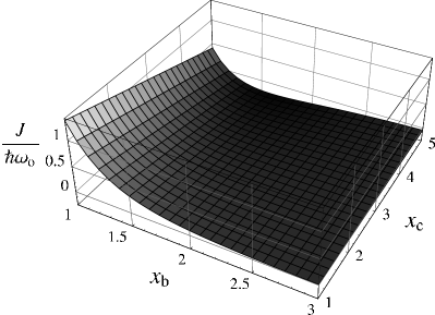
Figure 1: Plot of the exchange constant as a function of tunneling barrier and Coulomb energy in the case of three mutually interacting electrons (dimensionless units).

In Fig. 1, we plot the exchange-interaction constant $J$ in units of $\hbar\omega_{o}$ as a function of $x_{b}$ and $b_{c}$. The plot generally indicates that $J$ increases as the tunneling barrier decreases ($x_{b}$ smaller), an intuitively reasonable result. A negative minimum is visible when $x_{c}\sim 5$; this may reflect the breakdown of the HL approximation in the regime of strong interactions. Following Ref. D. Loss and D.P. DiVincenzo, 1998, we estimate that realistic values for GaAs heterostructure single dots, $x_{b}\sim 1$, $x_{c}\sim 1.5$, and $\hbar\omega_{o}=3\;\mathrm{meV}$, do not fall in this strong interactions regime.

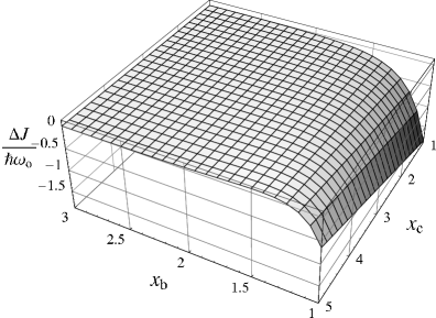
Figure 2: Plot of the change in the exchange constant due to $3$-electron-swap matrix elements. Horizontal axes as in Fig. 1 (with their directions flipped).

Fig. 2 shows the change $\Delta J$ that results from three-electron-swap matrix elements $\epsilon_{0}$ and $p_{0}$ (i.e. $\Delta J$ is the change in $J=2L_{1}$ when $\epsilon_{0}$ and $p_{0}$ are set to zero in expressions (4) and (5)). Comparing the scales of Figs. 1 and 2, one finds that the three-electron swap matrix elements can have a powerful influence on $J$. They will strongly impact quantum evolution when two-particle gates act simultaneously on three qubits (as may arise in circumstances (i) - (iii) above).

In the four electron case, a still more striking effect arises. Here, it is possible to have $S_{T}=0$, $S_{T}=1$, or $S_{T}=2$, so that one keeps three constants $L_{0}$, $L_{1}$, and $L_{2}$ in $H_{\mathrm{spin}}$. It follows immediately that $H_{\mathrm{spin}}$ includes terms of the form $L_{2}(\mathbf{S}_{A}\cdot\mathbf{S}_{B})(\mathbf{S}_{C}\cdot\mathbf{S}_{D})$ and permutations. Unless $L_{2}$ happens to vanish, the presence of a fourth electron introduces a qualitatively new 4-body interaction as well as a quantitative change in the exchange coupling between the other electrons.

We evaluate $L_{0}$, $L_{1}$, and $L_{2}$ using Eq. (3). Extending the three-electron definitions, we set

$$p_{0}=\left\langle BADC\right|ABCD\rangle, \epsilon_{0}=\left\langle BADC\right|H|ABCD\rangle,$$

$$p_{0}^{\prime}=\left\langle DABC\right|ABCD\rangle, \epsilon_{0}^{\prime}=\left\langle DABC\right|H\left|ABCD\right\rangle,$$

$$p_{1}=\left\langle ADBC\right|ABCD\rangle, \epsilon_{1}=\left\langle ADBC\right|H|ABCD\rangle,$$

$$p_{2}=\left\langle BACD\right|ABCD\rangle, \epsilon_{2}=\left\langle BACD\right|H|ABCD\rangle,$$

$$p_{4}=\left\langle ABCD\right|ABCD\rangle, \epsilon_{4}=\left\langle ABCD|H\right|ABCD\rangle.$$

A convenient state to use for $S_{T}=0$ is $|\Psi^{4}_{0}\rangle\propto\left(\left|\Psi(\uparrow\downarrow\uparrow\downarrow)\right\rangle-\left|\Psi(\uparrow\downarrow\downarrow\uparrow)\right\rangle-\left|\Psi(\downarrow\uparrow\uparrow\downarrow)\right\rangle+|\Psi(\downarrow\uparrow\downarrow\uparrow)\rangle\right)$. After normalization, this state yields the singlet energy

$$E_{0}=L_{0}=\frac{\epsilon_{4}-4\epsilon_{1}+3\epsilon_{0}}{p_{4}-4p_{1}+3p_{0}}.$$

A convenient state to use for $S_{T}=1$ is $|\Psi^{4}_{1}\rangle\propto\left(\left|\Psi(\uparrow\downarrow\uparrow\downarrow)\right\rangle+\left|\Psi(\uparrow\downarrow\downarrow\uparrow)\right\rangle-\left|\Psi(\downarrow\uparrow\uparrow\downarrow)\right\rangle-|\Psi(\downarrow\uparrow\downarrow\uparrow)\rangle\right)$. This state, after normalization, yields the triplet energy

$$E_{1}=L_{0}+2L_{1}+4L_{2}=\frac{\epsilon_{4}-2\epsilon_{2}-\epsilon_{0}+2\epsilon_{0}^{\prime}}{p_{4}-2p_{2}-p_{0}+2p_{0}^{\prime}}$$

Finally, a convenient state to use for $S_{T}=2$ is $|\Psi^{4}_{2}\rangle\propto\left|\Psi(\uparrow\uparrow\uparrow\uparrow)\right\rangle.$ We find for the quintet energy

$$E_{2}=L_{0}+6L_{1}+36L_{2}=\frac{\epsilon_{4}-6\epsilon_{2}+8\epsilon_{1}+3\epsilon_{0}-6\epsilon_{0}^{\prime}}{p_{4}-6p_{2}+8p_{1}+3p_{0}-6p_{0}^{\prime}}.$$

We would like to exhibit interaction constants explicitly in the spin Hamiltonian. Spin-operator identities allow one to convert from the form (2) to

$$H_{\mathrm{spin}} = K+J\sum_{i<j}\mathbf{S}_{i}\cdot\mathbf{S}_{j}+J^{\prime}[\left(\mathbf{S}_{A}\cdot\mathbf{S}_{B}\right)\left(\mathbf{S}_{C}\cdot\mathbf{S}_{D}\right)$$

$$+ \left(\mathbf{S}_{A}\cdot\mathbf{S}_{C}\right)\left(\mathbf{S}_{B}\cdot\mathbf{S}_{D}\right)+\left(\mathbf{S}_{A}\cdot\mathbf{S}_{D}\right)\left(\mathbf{S}_{B}\cdot\mathbf{S}_{C}\right)]$$

where $K=L_{0}+3L_{1}+\frac{27}{2}L_{2}$, $J=2L_{1}+14L_{2}$, and $J^{\prime}=8L_{2}$. Generically, $J^{\prime}$ does not vanish, and four-body interactions arise.

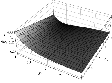
Figure 3: Plot of the exchange constant in the case of four mutually interacting electrons. Horizontal axes as in Fig. 1.

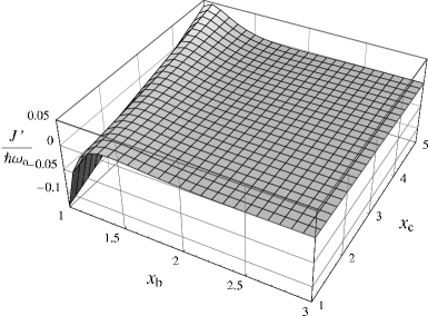
Figure 4: Plot of the $4$-body exchange constant in the case of four mutually interacting electrons. Horizontal axes as in Fig. 1.

We use the potential (7) to estimate the magnitude of the effect. The exchange-interaction constant $J$ is plotted in Fig. 3. Its form is similar to that of $J$ in the three-electron case, with a slightly reduced magnitude. The four-body interaction constant, $J^{\prime}$, appears in Fig. 4. In the parameter region of likely experimental interest ($x_{b}\sim 1$, $x_{c}\sim 1.5$, $\hbar\omega_{o}\sim 3\;\mathrm{meV}$), $J^{\prime}/J\sim-15\%$, certainly large enough to demand attention in computer design. Experimentally, four-body terms have been observed in ³He M. Roger (1983), and Cu₄O₄ square plaquettes in La₂CuO₄ R. Coldea, S.M. Hayden, G. Aeppli, T.G. Perring, C.D. Frost, T.E. Mason, S.-W. Cheong, and Z. Fisk (2001), where $J^{\prime}/J$ was found to be $\sim 27\%$.

Finally, to test the accuracy of our HL calculations, we have used a Hund-Mulliken (HM) calculation that extends the HL basis to include basis states with double occupation: two electrons on a single dot. For instance, the HM Hilbert space describing three electrons on three dots splits into a four-dimensional total-spin subspace with $S_{T}=3/2$ (same as in the HL case), and a $16$-dimensional $S_{T}=1/2$ subspace, comprised of two degenerate $S_{T,z}=\pm 1/2$ subspaces. For parameters of interest A.Mizel and D.A. Lidar (2003), twelve $S_{T}=1/2$ states have high energy and involve substantial double occupation while the remaining four $S_{T}=1/2$ states form a degenerate ground state similar to that of the HF basis. Therefore one recovers the HF picture by projecting out the $8$ lowest members of the HM solution (the four low $S_{T}=1/2$ and the four $S_{T}=3/2$ states) to obtain an exchange Hamiltonian (6). The corresponding $J$ qualitatively confirms the form of Fig. 1 and Fig. 2. Thus, even when HL results are not necessarily quantitatively precise, substantial many-body corrections to the interaction Hamiltonian persist in more accurate calculations. In the context of quantum computation, these effects could, on one hand, utterly derail an algorithm or, on the other, find uses in novel designs.