Steady state of atoms in a resonant field with elliptical polarization

Abstract

We present a complete set of analytical and invariant expressions for the steady-state density matrix of atoms in a resonant radiation field with arbitrary intensity and polarization. The field drives the closed dipole transition with arbitrary values of the angular momenta $J_{g}$ and $J_{e}$ of the ground and excited state. The steady-state density matrix is expressed in terms of spherical harmonics of a complex direction given by the field polarization vector. The generalization to the case of broad-band radiation is given. We indicate various applications of these results.

I Introduction

An atomic medium driven by a resonant light field represents a prototype problem in atomic physics and non-linear optics. At low density the effects of the atom-atom interaction are small, and the central remaining problem is specified by a single atom in a resonant radiation field. As is well-known, the basic processes are the absorption and emission of photons. The three universal conservation laws (energy, linear momentum and angular momentum) correspond to three different aspects in these processes. The main exchange of energy between atom and field corresponds to the radiative transition between the atomic energy levels. The momentum exchange gives rise to recoil of the atom, which is the basis of the mechanical action of light. The main angular momentum exchange arises from the photon spin. Its proper description requires consideration of the light polarization, and the degeneracy of atomic energy levels. Obviously, these processes occur simultaneously, and in a correlated fashion. The recoil effect is usually small, due to the smallness of the photon momentum ($\hbar k$) as compared to typical values of the atom momentum ($M\bar{v}$). In contrast, the (spin) angular momentum of photons $\hbar$ is of the same order of magnitude as the internal angular momentum of the atomic states.

A large fraction of theoretical studies of atoms in radiation fields only considers non-degenerate energy eigenstates, without taking into account the magnetic degeneracy of energy levels. In the sense of the group of space rotations, this approach corresponds to a scalar model of the atom, which accounts for exchange of energy and momentum, but not of angular momentum. This model allows to understand many processes arising from the resonant interaction of atoms with radiation [1, 2, 3, 4, 5]. However, effects of polarization in combination with the magnetic degeneracy of atomic levels cannot be ignored in many cases. The problem remains reasonably tractable in the special cases of linear or circular polarization. In these cases, there is an obvious choice of the quantization axis, so that the submatrices of the density matrix for the ground and the excited level remain diagonal at all times. For arbitrary elliptical polarization the situation is appreciably more complex. There are various experimental situations where elliptical polarization is quite essential. An important example is the phenomenon of coherent population trapping (CPT) of atoms driven by an elliptically polarized light field [6]. Another example is cooling and trapping of atoms in light fields with polarization gradients [7], where the strong correlation between the processes of linear and angular momentum exchange can lead to atom temperatures down to the single-photon recoil energy ($\sim 10^{-6}K$). Here continuous spatial variations of the polarization are crucial, which, except for special cases, give rise to elliptical polarization. Models with non-degenerate atomic states can only describe the Doppler limit of laser cooling ($\sim 10^{-3}K$) [5].

A central part of these processes is the resonant interaction of an elliptically polarized light field with a closed atomic transition between degenerate energy levels. In this case the light-induced anisotropy of the atomic state is long-lived. This enables one to accumulate information on very weak couplings, which allows for high-resolution spectroscopy. As noted above, for many cases one can consider the recoil effect as a small perturbation of the order of $\hbar k/M\bar{v}\ll 1$. In zeroth order the atom has a constant linear momentum. In this case only the exchange of energy and angular momentum between atom and field is taken into account, and the state of the atom is fully described by the density matrix for the internal states. The remaining field effects (light shifts, field broadening, change of population and coherence etc.) are caused by the stimulated and spontaneous transitions, which are described by the generalized optical Bloch equations (GOBE) for the internal atomic density matrix. Depending on the light intensity and interaction time, three limiting cases can be distinguished. The first case occurs for short light pulses, when the interaction time is so short that relaxation processes can be neglected. Then the interaction of atoms with the field has a coherent character, and it can be described by the time-dependent Schrödinger equation for the atomic wavefunction. Typical effects are coherent transient processes, such as Rabi oscillations or photon echoes, which have been thoroughly analyzed [1, 8], with or without inclusion of the magnetic degeneracy of atomic states [9]. The second case occurs when the interaction time is long compared with the spontaneous lifetime, but still short compared with the absorption time, which determines the rate of optical pumping. In this case one can use perturbation theory. This situation arises for laser beams of low intensity and small diameter, when time-of-flight effects become important. Solutions of the optical Bloch equations corresponding to this case have been obtained with the use of irreducible-tensor techniques for arbitrary Zeeman and hyperfine level structures [10]. Finally, when the interaction time is so long that perturbation theory becomes inapplicable, one has to find the steady-state solution of the GOBE. This situation appears either for slow atoms interacting with light, such as in optical molasses, or in the case of light beams with high intensity or large diameter. A common restriction is that only a closed transition between two degenerate atomic levels is considered, so that the total population is conserved.

The GOBE are an essential ingredient of the description of sub-Doppler laser cooling by fields with polarization gradients [11]. We here recall just a few representative cases. In the semiclassical theory of laser cooling authors concentrated their efforts on the velocity-dependent steady-state density matrix. The presented analytical results were, however, restricted to transitions with specific small values of the angular momenta of the states [12]. Berman et al. [13] have formulated the GOBE for arbitrary field polarization and arbitrary atomic energy level structure, using the irreducible tensor representation. They demonstrate that the sub-Doppler light forces and the sub-natural resonances in non-linear spectroscopy are closely related. Similar results have been obtained in [14], where a general relationship between the light force and the non-linear polarizability tensor has been derived.

For linear or circular polarization, the steady-state solutions of the GOBE have been discussed in various papers [15, 16, 17] for arbitrary values of $J_{g}$ and $J_{e}$. For arbitrary polarization, the symmetry is reduced, and the steady state for arbitrary $J_{g}$ and $J_{e}$ represents a complex mathematical problem. The number of equations, which is equal to the number of elements of the density matrix, amounts to $4(J_{g}+J_{e}+1)^{2}$. The steady-state density matrix was found in analytical form only for transitions involving specific small values of the angular momentum ($J_{g}=0,\,1/2,\,1$) [18, 19, 20, 21, 22]. Recently we have discussed the steady state of atoms in light fields with arbitrary polarization, for transitions with $J_{e}-J_{g}=0$ [23, 24] or $1$ [25]. In these cases, the structure of the solutions looked remarkably different. An invariant approach to the general problem, based on the expansion of the density matrix in bipolar harmonics of complex directions was developed in [26]. Nasyrov [27] has suggested an alternative approach to the steady-state density matrix, using the semiclassical Wigner representation of angular-momentum orientation . This method seems especially useful at large angular momentum $J\gg 1$. The results are in good qualitative agreement with our exact solution.

In the present paper we give unified exact analytical expressions for the steady state of atoms driven by light with an arbitrary polarization, for all possible dipole transitions. Radiative relaxation is included in the description, and the results are presented in an invariant form. The analysis is based upon the group-theoretical properties of the transition dipole. The polarization direction in real space is reflected in the density matrix for the two subspaces corresponding to the ground and excited state. The symmetry group for the problem is the group of rotations $SU(2)$, which is an important leading principle for the search of the solution, as well as for its presentation in invariant form. The general discussion allows us to clarify the similarities in the different cases, which were not obvious at all in the separate treatments.

The nature of the steady state strongly depends on the value of $J_{e}-J_{g}$. For dipole-allowed transitions, this difference can be $-1$, $0$ or $1$. For the case that $J_{e}=J_{g}=J$ we should moreover distinguish the cases that $J$ is integer or half-integer. This leads to four classes of transitions.

• Transitions $J_{g}=J\rightarrow J_{e}=J-1$. In this case atoms are optically pumped into dark states, where they do not couple to the light field. This is the phenomenon of coherent population trapping. These dark states are linear superpositions of the Zeeman substates of the ground level, defined as eigenstates of the resonant interaction Hamiltonian with zero eigenvalue. Hence, there are no light shifts. For the present class of transitions, there are two independent dark states, which span a two-dimensional space. This space depends only on the polarization, and it is independent of the field intensity and the detuning. Both the atomic dynamics in the field and the steady state depend on the initial state.

• Transitions $J_{g}=J\rightarrow J_{e}=J$ with $J$ integer. In this case a single dark state exists, and CPT takes place, so that in the steady state the atom is in this unique pure state. Therefore, the steady state does not depend on the initial conditions, the intensity or the detuning.

• Transitions $J_{g}=J\rightarrow J_{e}=J$ with $J$ half-integer. For this class no dark state exists, and CPT does not occur. The only exception is the case of circular polarization, where a single dark state does occur. The steady state is uniquely defined, but now it depends both on the polarization, the intensity and the detuning. Moreover, it is not a pure state. In fact, it has the remarkable property that the excited-state submatrix of the density matrix is fully isotropic, which makes the analytical expression for the entire density matrix particularly simple.

• Transitions $J_{g}=J\rightarrow J_{e}=J+1$. For this class of transitions the steady-state solution is unique. There is no dark state. The excited-state submatrix is always anisotropic.

Only in the cases c) and d) does a steady-state excitation exist. In both cases, the anisotropy of the excited state and of the optical coherences depends only on the polarization of the driving field. The intensity and the detuning enter only as an overall multiplicative factor. Moreover, in both cases we find that the submatrices both for the excited and the ground state are even functions of the detuning. In the cases a) and b) only the ground state is populated in the steady state, and the excited-state submatrix and the optical coherences vanish. The occurrence of dark states and velocity-selective CPT allows to reach cooling below the recoil limit [28], and it has been studied by many authors [29]. In the case of $J_{g}=1$ an invariant form of the dark states in an elegant vector notation has been used for the analysis of CPT in 2D and 3D [30]. Here we extend an invariant approach to all the dark transitions.

The remainder of the paper is organized as follows. First we discuss the general structure of the generalized optical Bloch equations (Sec. II), which leads in Sec. III to the definition of a natural basis of states that depend only on the light polarization. We separately discuss the cases with (Sec. IV) or without (Sec. V) dark states. In the latter case, we discuss the effect of optical pumping on the degree of excitation and the AC Stark shift in Sec. VI. The generalization to the situation of broad-band radiation is given in Sec. VII.

II Formulation of the problem

We consider a closed atomic transition $J_{g}\rightarrow J_{e}$ with a transition frequency $\omega_{0}$ of an atom at a given position. In the present paper we will not consider the translational motion of the atom. This corresponds either to the case of very slow atoms or to the case of a travelling plane wave, where the atomic motion at a given velocity leads only to a Doppler frequency shift. The transition is driven by a monochromatic radiation field with frequency $\omega$ and arbitrary polarization ${\bf e}$. The time-dependent electric field vector at the position of the atom is given by

$${\bf E}=E_{0}{\bf e}\exp(-i\omega t)+c.c.$$ (1)

where the polarization vector is

$${\bf e}=\sum_{q=0,\pm 1}e_{q}{\bf e}_{q}^{*}\;=\sum_{q=0,\pm 1}(-1)^{q}e_{-q}{\bf e}_{q}.$$ (2)

Here $E_{0}$ is the complex field amplitude, $e_{q}={\bf e}\cdot{\bf e}_{q}$ is the covariant spherical component of the polarization vector ${\bf e}$, and the spherical basis vectors of polarization are defined by $\{{\bf e}_{0}={\bf e}_{z};\;{\bf e}_{\pm 1}={\mp}({\bf e}_{x}\pm i{\bf e}_{y})/\sqrt{2}\}$. Notice that ${\bf e}_{q}^{*}=(-1)^{q}{\bf e}_{-q}$. The vector ${\bf e}$ is normalized, so that ${\bf e}^{*}\cdot{\bf e}=1$ and without loss of generality we assume that its real and imaginary parts are orthogonal, which implies that $\mbox{Im}({\bf e}\cdot{\bf e})=0$. Then the two vectors $\mbox{Re}\;{\bf e}$ and $\mbox{Im}\;{\bf e}$ are the axes of the polarization ellipse.

It is always possible to use a coordinate frame where only two of the components $e_{q}$ are nonzero. There are two possibilities. The conventional choice is that the $Oz$ axis is chosen normal to the polarization plane. In this coordinate system the vector ${\bf e}$ is the sum of the two opposite circular unit vectors ${\bf e}_{\pm 1}$. If the $Ox$ axis is directed along the major semiaxis of the polarization ellipse (see Fig. 1a), ${\bf e}$ is written as

$\displaystyle{\bf e}={\bf e}_{x}\;\cos{\varepsilon}+i{\bf e}_{y}\;\sin{\varepsilon}=-{\bf e}_{+1}\;\sin{(\varepsilon+\pi/4)}+{\bf e}_{-1}\cos{(\varepsilon+\pi/4)}\,,$

where the ellipticity angle $\varepsilon$ can take the values $-\pi/4\leq\varepsilon\leq\pi/4$. Obviously, $|\tan\,\varepsilon|$ is equal to the ratio of the minor semiaxis to the major semiaxis and the sign of $\varepsilon$ determines the helicity.

Another choice is called the natural coordinate frame, which was introduced in [31]. When we represent the polarization ellipse as the intersection of a cylinder with a plane, the natural frame $Ox^{\prime}y^{\prime}z^{\prime}$ is specified by the requirement that the axis $Oz^{\prime}$ is the axis of the cylinder, while the axis $Oy^{\prime}$ coincides with the axis $Oy$. The minor semiaxis of the ellipse coincides with the radius of the cylinder (Fig. 2a). Then the polarization ${\bf e}$ is the superposition of a linear component along $Oz^{\prime}$, and one circular component. The two frames are connected by a rotation along the axis $Oy$ over an angle $\theta$ obeying the relation

$\displaystyle\cos{\theta}=|\tan\,{\varepsilon}|\,.$

In the natural frame, the polarization vector is specified as

$${\bf e}={\bf e}_{0}^{\prime}\sqrt{\cos(2\varepsilon)}-{\bf e}_{\pm 1}^{\prime}\sqrt{2}\sin(\varepsilon),$$ (3)

where the helicity of the spherical unit vector ${\bf e}_{\pm 1}^{\prime}$ corresponds to the sign of $\varepsilon$. In general there are two possible choices for the cylinder, corresponding to opposite signs of the rotation angle $\theta$. Notice that when the polarization ${\bf e}$ is represented in terms of the Stokes vector as a point on the Poincaré sphere, the angle $\theta$ is equal to the polar angle of this point [32].

The quantum kinetic equation for the density matrix $\widehat{\rho}$ of the internal state of the atom in the external field (1) has the form:

$$\frac{\partial}{\partial t}\widehat{\rho}=-\frac{i}{\hbar}\left[\widehat{H}_{0},\widehat{\rho}\right]-\frac{i}{\hbar}\left[-\widehat{{\bf d}}\cdot{\bf E}(t),\widehat{\rho}\right]-\widehat{\Gamma}\{\widehat{\rho}\}\;.$$ (4)

Here $\widehat{H}_{0}$ is the Hamiltonian describing the energy of the two resonant levels of the free atom and $\widehat{{\bf d}}$ is the dipole operator connecting the two levels. The radiative relaxation is described by the operator $\widehat{\Gamma}\{\widehat{\rho}\}$. All operators are represented as matrices on the Zeeman basis of the ground and excited levels, with states $\{|J_{g},\mu_{g}\rangle\}$ and excited $\{|J_{e},\mu_{e}\rangle\}$. The density matrix $\widehat{\rho}$ can be separated in four matrix blocks, where the matrices $\widehat{\rho}_{gg}$ and $\widehat{\rho}_{ee}$ are the submatrices for the ground and excited state, and the off-diagonal blocks $\widehat{\rho}_{eg}$ and $\widehat{\rho}_{ge}$ describe the optical coherences. In the rotating-wave approximation the time dependence of the kinetic equation can be removed by introducing the transformed optical coherences as

$$\widehat{\rho}_{eg}=\exp(-i\omega t)\widehat{\overline{\rho}}_{eg}\;\;\;\;\widehat{\rho}_{ge}=\exp(i\omega t)\widehat{\overline{\rho}}_{ge}.$$ (5)

The resulting system of generalized optical Bloch equations (GOBE) can be expressed in the dimensionless dipole operator $\widehat{{\bf D}}$, which couples the ground state to the excited state. It is specified by the definition of its spherical components as

$$\widehat{D}_{q}\equiv\widehat{{\bf D}}\cdot{\bf e}_{q}=\sum_{(\mu)}|J_{e},\mu_{e}\rangle\,C_{J_{g}\,\mu_{g}\;1\,q}^{J_{e}\,\mu_{e}}\,\langle J_{g},\mu_{g}|\,,$$ (6)

so that their matrix elements are equal to the Clebsch-Gordan coefficients $C_{J_{g}\,\mu_{g}\;1\,q}^{J_{e}\,\mu_{e}}$. Stimulated transitions are described by the operator $\widehat{V}$, which is the component of the vector operator $\widehat{{\bf D}}$ in the polarization direction:

$$\widehat{V}=\widehat{{\bf D}}\cdot{\bf e}\,.$$ (7)

Then the GOBE take the form

$$\left(\frac{\partial}{\partial t}+\frac{\gamma}{2}-i\delta\right)\widehat{\overline{\rho}}_{eg}=i\Omega\left[\widehat{V}\widehat{\rho}_{gg}-\widehat{\rho}_{ee}\widehat{V}\right]$$ (8)

$$\left(\frac{\partial}{\partial t}+\frac{\gamma}{2}+i\delta\right)\widehat{\overline{\rho}}_{ge}=i\Omega^{*}\left[\widehat{V}^{\dagger}\widehat{\rho}_{ee}-\widehat{\rho}_{gg}\widehat{V}^{\dagger}\right]$$ (9)

$$\left(\frac{\partial}{\partial t}+\gamma\right)\widehat{\rho}_{ee}=i\left[\Omega\widehat{V}\widehat{\overline{\rho}}_{ge}-\Omega^{*}\widehat{\overline{\rho}}_{eg}\widehat{V}^{\dagger}\right]$$ (10)

$$\frac{\partial}{\partial t}\widehat{\rho}_{gg}-\gamma\sum_{q=0,\pm 1}\widehat{D}_{q}^{\dagger}\,\widehat{\rho}_{ee}\,\widehat{D}_{q}=i\left[\Omega^{*}\widehat{V}^{\dagger}\widehat{\overline{\rho}}_{eg}-\Omega\widehat{\overline{\rho}}_{ge}\widehat{V}\right],$$ (11)

with the normalization

$${\rm Tr}\{\widehat{\rho}_{gg}\}+{\rm Tr}\{\widehat{\rho}_{ee}\}=1.$$ (12)

Here $\delta=\omega-\omega_{eg}$ is the detuning, $\omega_{eg}=(E_{e}-E_{g})/\hbar$ is the transition frequency, $\gamma$ is the radiation relaxation rate and $\Omega=E_{0}\langle J_{e}||d||J_{g}\rangle/\hbar$ is the generalized Rabi frequency, expressed in the complex field amplitude $E_{0}$ and the reduced dipole matrix element $\langle J_{e}||d||J_{g}\rangle$ that determines the strength of the transition. The summation in eq. (11), which describes the feeding of the ground state by spontaneous decay, runs over the three possible independent polarizations $\{{\bf e}_{0},{\bf e}_{\pm 1}\}$ of spontaneous emission. Conservation of the total population of the closed transition is ensured by the relation

$$\sum_{q=0,\pm 1}\widehat{D}_{q}\,\widehat{D}_{q}^{\dagger}=\widehat{\Pi}_{e}\;.$$ (13)

When acting on an isotropic excited state, this feeding term is proportional to

$$\sum_{q=0,\pm 1}\widehat{D}_{q}^{\dagger}\,\widehat{D}_{q}=\frac{2J_{e}+1}{2J_{g}+1}\,\widehat{\Pi}_{g}\,.$$ (14)

We introduced $\widehat{\Pi}_{g}$ and $\widehat{\Pi}_{e}$ as the projectors on the ground state and the excited state. The dynamical equations (8)-(11) represent the generalized optical Bloch equations, which describe transient processes as generalized damped Rabi oscillations, optical nutation, free induction decay, etc., as well as optical pumping effects, that lead to an anisotropic distribution of atoms over the magnetic sublevels.

Equations for the steady state are obtained by setting all time derivatives to zero in eqs. (8)-(11), which gives a set of linear equations for the density-matrix elements. By using eqs. (8) and (9), the steady-state optical coherences can be directly expressed in the population submatrices $\widehat{\rho}_{ee}$ and $\widehat{\rho}_{gg}$ as

$\displaystyle\widehat{\overline{\rho}}_{eg}=\frac{-i\Omega}{\gamma/2-i\delta}\left[\widehat{V}\widehat{\rho}_{gg}-\widehat{\rho}_{ee}\widehat{V}\right]\;,$

$$\widehat{\overline{\rho}}_{ge}=\frac{-i\Omega^{*}}{\gamma/2+i\delta}\left[\widehat{V}^{\dagger}\widehat{\rho}_{ee}-\widehat{\rho}_{gg}\widehat{V}^{\dagger}\right].$$ (15)

After substitution in (10) and (11), this leads to closed equations for the population submatrices in the form

$$\gamma\widehat{\rho}_{ee}=-\gamma S/2\{\widehat{V}\widehat{V}^{\dagger},\widehat{\rho}_{ee}\}+\gamma S\widehat{V}\widehat{\rho}_{gg}\widehat{V}^{\dagger}+i\delta S[\widehat{V}\widehat{V}^{\dagger},\widehat{\rho}_{ee}]\;,$$ (16)

$$-\gamma\sum_{q=0,\pm 1}\widehat{D}_{q}^{\dagger}\widehat{\rho}_{ee}\widehat{D}_{q}=-\gamma S/2\{\widehat{V}^{\dagger}\widehat{V},\widehat{\rho}_{gg}\}+\gamma S\widehat{V}^{\dagger}\widehat{\rho}_{ee}\widehat{V}-i\delta S[\widehat{V}^{\dagger}\widehat{V},\widehat{\rho}_{gg}];$$ (17)

where $\{\,,\,\}$, $[\,,\,]$ indicate an anticommutator and a commutator, respectively, and where

$$S=\frac{|\Omega|^{2}}{\gamma^{2}/4+\delta^{2}}$$ (18)

is the saturation parameter, which is proportional to the light intensity and to the global oscillator strength of the transition. The left-hand sides of eqs. (16) and (17) describe spontaneous processes, i.e. the radiative damping of the excited level and the spontaneous transfer of population and Zeeman coherence from the excited to the ground level. The terms in the right-hand sides that are proportional to the optical pumping rate $\gamma S$ represent light-induced loss (with the minus sign) and gain (with the plus sign) of the levels. The commutator terms in the right-hand sides, proportional to $\delta S$, describe the AC Stark effect. They contain the light-shift operators in the ground and excited level

$$\widehat{{\cal E}}_{g}=\delta S\widehat{V}^{\dagger}\widehat{V}\;,\;\widehat{{\cal E}}_{e}=-\delta S\widehat{V}\widehat{V}^{\dagger}\,,$$ (19)

which play the role of an effective Hamiltonian for the two levels.

The steady-state solution of the GOBE corresponds to the limit $t\to\infty$, with $t$ the interaction time. In practice this means that $t$ is larger than the largest relaxation time in the internal degrees of freedom. In the case of a degenerate ground state at low saturation this largest time is of the order of $(\gamma S)^{-1}$, which is the inverse of the rate of optical orientation in the ground state. For large saturations $S>1$ the largest relaxation time is the excited-state lifetime $\gamma^{-1}$. Thus, the conditions for the steady-state regime can be written as

$${\rm min}\{\gamma t,\gamma St\}\gg 1\,.$$ (20)

III Natural basis of states

A Commutation of density matrix and light-shift operators

In the special case of linear or circular polarization, the Zeeman substates $|J_{g},\mu_{g}\rangle$ and $|J_{e},\mu_{e}\rangle$ constitute an obvious natural basis of substates in which to express the density matrix. For linear polarization, one chooses the quantization axis parallel to the polarization direction, so that the polarization vector ${\bf e}$ is equal to the spherical unit vector ${\bf e}_{q}$ with $q=0$. For circular polarization, the polarization vector ${\bf e}$ is equal to the spherical unit vector ${\bf e}_{q}$ with $q=\pm 1$, provided that the quantization axis is chosen normal to the polarization plane. In both cases, the operator $\widehat{V}$ couples each substate $|J_{g},\mu_{g}\rangle$ to a single excited state $|J_{e},\mu_{e}\rangle$, which $\mu_{e}=\mu_{g}$ (linear polarization) or $\mu_{e}=\mu_{g}\pm 1$ (circular polarization). In this case it can be easily checked from eqs. (8)-(11) that the equations for the populations do not mix with those for the Zeeman coherences. Also, eqs. (16) and (17) show that the steady-state solutions $\widehat{\rho}_{ee}$ and $\widehat{\rho}_{gg}$ are diagonal on the basis of the Zeeman substates $|J,\mu\rangle$. Since also the light-shift operators $\widehat{{\cal E}}_{g}$ and $\widehat{{\cal E}}_{e}$ are diagonal on the Zeeman substates, this implies that the steady-state density matrices $\widehat{\rho}_{gg}$ and $\widehat{\rho}_{ee}$ commute with the light-shift operators $\widehat{{\cal E}}_{g}$ and $\widehat{{\cal E}}_{e}$, so that for linear or circular polarization we find

$$[\widehat{\rho}_{gg},\widehat{{\cal E}}_{g}]=0\;,\;\;\;[\widehat{\rho}_{ee},\widehat{{\cal E}}_{e}]=0\;.$$ (21)

Moreover, when all Zeeman coherences are zero initially at $t=t_{0}$, they remain zero for all later times $t>t_{0}$.

One might be tempted to believe that also for arbitrary elliptical polarization a basis of states can be chosen for which populations and coherences do not mix. However, this is not true. It has been shown in ref. [33] that spontaneous decay can create coherence between eigenstates of $\widehat{{\cal E}}_{g}$, even if they do not exist initially. In general the time-dependent solutions $\widehat{\rho}_{gg}$ and $\widehat{\rho}_{ee}$ for arbitrary polarization will not commute with the light-shift operators at all times.

Nevertheless, in this paper we shall prove that for the steady-state solutions for all classes of transitions the commutation rules (21) are valid for arbitrary elliptical polarization and for all classes of transitions. The proof is rather different for the various classes, so that it is most convenient to give the proof while discussing the expression for the steady state for each class separately. An immediate consequence of the commutation rules (21) is that the steady-state density matrix is diagonal in the eigenstates of the light-shift operators. This implies also that the last terms in eqs. (16) and (17) vanish, so that the steady-state population submatrices depend on the detuning $\delta$ and the spontaneous-decay rate $\gamma$ only through the saturation parameter $S$.

B Eigenbasis of light-shift operators

We are interested in the eigenstates of the operators $\widehat{V}^{\dagger}\widehat{V}$ and $\widehat{V}\widehat{V}^{\dagger}$. The corresponding eigenvalues are real and non-negative, so that we can write

$$\widehat{V}^{\dagger}\widehat{V}|(g)i\rangle=\lambda_{i}^{2}|(g)i\rangle\,;\;\;\widehat{V}\widehat{V}^{\dagger}|(e)j\rangle=\lambda_{j}^{2}|(e)j\rangle$$ (22)

with $\lambda_{i}$ real, and with eigenstates $|(g)i\rangle$ in the ground and $|(e)j\rangle$ in the excited level. For given values of $J_{e}$ and $J_{g}$, the eigenstates and eigenvalues are fully determined by the polarization of the driving field, and they do not depend on the detuning or the intensity. The states $|(e)j\rangle$ and $|(g)i\rangle$ form the natural bases for the excited and the ground level. The operators $\widehat{{\cal E}}_{g}$ and $\widehat{{\cal E}}_{e}$ are diagonal with diagonal elements $\delta S\lambda_{i}^{2}$ and $-\delta S\lambda_{j}^{2}$. Operating with the coupling matrices $\widehat{V}$ and $\widehat{V}^{\dagger}$ on the first equation (22) shows that $\widehat{V}|(g)i\rangle$ is eigenstate of $\widehat{V}\widehat{V}^{\dagger}$ with eigenvalue $\lambda_{i}^{2}$. Hence we may assume that $\widehat{V}|(g)i\rangle$ is proportional to $|(e)i\rangle$. A proper choice of the phases of the eigenstates $|(e)i\rangle$ then leads to the expression

$$\widehat{V}=\sum_{i}\lambda_{i}|(e)i\rangle\langle(g)i|\;.$$ (23)

Hence each non-zero value of $\lambda_{i}$ corresponds to a pair of states $|(g)i\rangle$ and $|(e)i\rangle$ that are coupled by $\widehat{V}$ and $\widehat{V}^{\dagger}$. In addition, the operator $\widehat{V}^{\dagger}\widehat{V}$ or $\widehat{V}\widehat{V}^{\dagger}$ may have eigenvalues zero. The corresponding eigenstates are unaffected by the radiation field, and they do not contribute to the coupling operator (23).

If the commutation rules (21) are true, the steady-state density matrices $\widehat{\rho}_{gg}$ and $\widehat{\rho}_{ee}$ are diagonal on these bases. The diagonal elements $\pi_{i}^{(g)}$ and $\pi_{j}^{(e)}$ are the stationary populations. Taking the diagonal elements of the equations (16) and (17), we obtain the relations

$$\gamma\pi_{i}^{(e)}=-\gamma S\lambda_{i}^{2}\pi_{i}^{(e)}+\gamma S\lambda_{i}^{2}\pi_{i}^{(g)}$$ (24)

$$-\gamma\sum_{j}{\cal W}_{ij}\pi_{j}^{(e)}=-\gamma S\lambda_{i}^{2}\pi_{i}^{(g)}+\gamma S\lambda_{i}^{2}\pi_{i}^{(e)}\,$$ (25)

for the steady-state populations, with

$\displaystyle{\cal W}_{ij}=\sum_{q=0,\pm 1}\left|\langle(e)j|\widehat{D}_{q}|(g)i\rangle\right|^{2}\,$

the probabilities of the spontaneous transitions $j\to i$. These transition probabilities are normalized as $\sum_{i}{\cal W}_{ij}=1$ for all $j$. As is seen from (24), if $\widehat{{\cal E}}_{e}$ has an eigenvalue equal to zero, then the corresponding eigenstate $|(e)j\rangle$ is not populated. Conversely, if one or more eigenvalues $\lambda_{i}^{2}$ of $\widehat{{\cal E}}_{g}$ are equal to zero, then a steady state exists where only the corresponding eigenstates $|(g)i\rangle$ of the ground level are populated. For $\lambda_{j}\neq 0$ it follows from (24) that the populations of the ground- and excited-level substates are related by the equation

$$\pi_{j}^{(g)}=(1+\frac{1}{S\lambda_{j}^{2}})\pi_{j}^{(e)}\,.$$ (26)

From (25), it then follows that one can deduce a closed system of equations for the excited-state populations in the form

$$\sum_{j}{\cal W}_{ij}\pi_{j}^{(e)}=\pi_{i}^{(e)}\,.$$ (27)

These relations (27) uniquely determine the populations $\pi_{i}^{(e)}$, apart from normalization. This implies that the steady-state density matrix of the excited level $\widehat{\rho}_{ee}$ depends on the intensity and the detuning only through a normalization constant, which is a function of the saturation parameter $S$. Moreover, they show that the distribution over the excited-level substates can be considered as a stationary point of the radiative relaxation operator, in the sense that such a distribution is invariant under spontaneous decay to the ground level [34].

C Condition for diagonal steady state

The conjecture of the commutation relations (21) can be formulated in an invariant form. It is sufficient to assume the existence of two Hermitian operators $\widehat{E}$ and $\widehat{G}$, with $\widehat{E}$ acting on the excited states, and $\widehat{G}$ on the ground states, and obeying the identities

$$\widehat{E}\widehat{V}=\widehat{V}\widehat{G}\;\;,\;\;\sum_{q=0,\pm 1}\widehat{D}_{q}^{\dagger}\widehat{E}\widehat{D}_{q}=\widehat{G}\;\;.$$ (28)

From the first identity (28) it follows that the operators $\widehat{E}$ and $\widehat{G}$ have an identical diagonal matrix form on the natural bases. From this identity and its Hermitian conjugate $\widehat{V}^{\dagger}\widehat{E}=\widehat{G}\widehat{V}^{\dagger}$ one obtains the commutaton rules

$$[\widehat{E},\widehat{V}\widehat{V}^{\dagger}]=0\;\;,\;\;[\widehat{G},\widehat{V}^{\dagger}\widehat{V}]=0\;.$$ (29)

Starting from the relations (28), while using the equations (16) and (17), one easily derives that the steady-state submatrices $\widehat{\rho}_{ee}$ and $\widehat{\rho}_{gg}$ are determined by the relations

$$\widehat{\rho}_{ee}=\beta S\widehat{E}\;\;,\;\;\widehat{V}^{\dagger}\widehat{V}\widehat{\rho}_{gg}=\beta\left(1+S\widehat{V}^{\dagger}\widehat{V}\right)\widehat{G}\;\;,$$ (30)

with $\beta$ a normalization constant. These relations are just the operator expression of eq. (26). From (29) and (30) it follows immediately that the commutation rules (21) hold, and that the density matrix is diagonal on the natural basis. Therefore, the problem of finding expressions for the steady-state density matrix is now reduced to finding operators $\widehat{E}$ and $\widehat{G}$ that obey the relations (28). These operators can be assumed to depend only on the polarization vector ${\bf e}$, and not on the intensity or the detuning. When operators $\widehat{E}$ and $\widehat{G}$ obeying (28) are found, the steady-state density matrix is determined by (30), and it is indeed diagonal in the natural basis.

IV Dark states

As recalled in the Introduction, dipole transitions can be classified into two classes depending on the occurrence of coherent population trapping (CPT). For the first group, where CPT occurs, one or more of the eigenvalues of the ground-state light-shift operator $\widehat{{\cal E}}_{g}$ vanish, so that this operator cannot be inverted. During the optical-pumping process atoms are accumulated in the corresponding eigenstates, which are termed dark states, since they do not interact with the light field. Then the trivial solution $\widehat{E}=\widehat{G}=0$ of the system (28) still determines a normalizable steady-state solution of the relations (30) obeying $\widehat{\rho}_{ee}=0$ and $\widehat{V}^{\dagger}\widehat{V}\widehat{\rho}_{gg}=0$. The ground-state density matrix $\widehat{\rho}_{gg}$ is composed of the ground-level dark states $|\Psi^{(NC)}\rangle$, which obey the equation

$$\widehat{V}\,|\Psi^{(NC)}\rangle=0\,.$$ (31)

In order to specify the dark states in an invariant manner, we view state vectors as tensors. A state vector $|\Psi\rangle$ in the ground level is considered as a tensor $\Psi_{J_{g}}$ of the rank $J_{g}$, with (covariant) components $\Psi_{J_{g}\,-\mu_{g}}$ specified by the expansion

$\displaystyle|\Psi\rangle=\sum_{\mu_{g}}(-1)^{-\mu_{g}}\Psi_{J_{g}\,-\mu_{g}}\left|J_{g},\mu_{g}\right\rangle\;.$

Using the Wigner-Eckart theorem, we express the matrix elements of the left-hand side of eq. (31) as

$$\langle J_{e},\mu_{e}|(\widehat{{\bf d}}\cdot{\bf e})|\Psi^{(NC)}\rangle = \langle J_{e}||d||J_{g}\rangle\sum_{q,\mu_{g}}C_{J_{g}\mu_{g}\,1q}^{J_{e}\mu_{e}}(-1)^{-q}e_{-q}(-1)^{-\mu_{g}}\Psi_{J_{g}\,-\mu_{g}}^{(NC)}$$

$$= \langle J_{e}||d||J_{g}\rangle(-1)^{-\mu_{e}}\{{\bf e}\otimes\Psi_{J_{g}}^{(NC)}\}_{J_{e}\,-\mu_{e}}\;,$$

where $\{\ldots\otimes\ldots\}$ denotes the standard definition of an irreducible tensor product [35], $\langle J_{e}||d||J_{g}\rangle$ is the reduced matrix element of the dipole moment operator, and as before, $e_{q}={\bf e}\cdot{\bf e}_{q}$ is the covariant spherical component of the polarization vector ${\bf e}$. The invariant expression of eq. (31) in terms of a tensor product of rank $J_{e}$ reads

$$\{{\bf e}\otimes\Psi_{J_{g}}^{(NC)}\}_{J_{e}}=0\,,$$ (32)

with the normalization condition $({\Psi_{J_{g}}^{(NC)}}^{*}\cdot\Psi_{J_{g}}^{(NC)})=1\,.$

A Transitions $J_{g}=J\rightarrow J_{e}=J$ with integer $J$

For transitions with integer values of $J_{g}=J_{e}=J$ there is a single dark state for any polarization [6]. In order to write an explicit and invariant form of $\Psi^{(NC)}_{J}$ in this case, we introduce the $L$-fold tensor product of the vector ${\bf e}$ [36, 37]

$$\{{\bf e}\}_{L}=\{\ldots\{\{{\bf e}\otimes{\bf e}\}_{2}\otimes{\bf e}\}_{3}\,...\otimes{\bf e}\}_{L}\,.$$ (33)

which are proportional to the spherical harmonics of a complex direction $n_{LM}({\bf e})$ (Appendix A). Notice that the three components $\{e\}_{1q}$ in the case $L=1$ coincide with the spherical components of the (possibly complex) vector ${\bf e}$.

The Clebsch-Gordan expansion (A.3) for a product of two spherical harmonics with the same argument leads to the result

$$\{\{{\bf e}\}_{L}\otimes\{{\bf e}\}_{J}\}_{K}=C_{L0\,J0}^{K0}\,\sqrt{\frac{L!\,J!\,(2K-1)!!\,({\bf e}\cdot{\bf e})^{L+J-K}}{K!\,(2L-1)!!\,(2J-1)!!}}\,\{{\bf e}\}_{K}\,.$$ (34)

It follows from the symmetry of the Clebsch-Gordan coefficients that $C_{L0\,J0}^{K0}=0$ if $L+J-K$ is odd. Then choosing $L=1$ and $K=J$ we obtain $\{{\bf e}\otimes\{{\bf e}\}_{J}\}_{J}=0$, so that the single dark state as defined by (32) can be specified in tensor form as

$$\Psi_{J}^{(NC)}={\cal N}\{{\bf e}\}_{J}\,.$$ (35)

The normalization constant follows from the equality

$$(\{{\bf e}\}_{J}\cdot\{{\bf e}^{*}\}_{J})=\frac{J!}{(2J-1)!!}({\bf e}\cdot{\bf e})^{J/2}({\bf e}^{*}\cdot{\bf e}^{*})^{J/2}\,P_{J}\left(\frac{({\bf e}\cdot{\bf e}^{*})}{({\bf e}\cdot{\bf e})}\right)\,,$$ (36)

as an example of the sum rule for spherical harmonics (A.4). Here $P_{J}(x)$ is the standard notation for Legendre polynomials. This leads to the expression

$${\cal N}=\left[\frac{J!}{(2J-1)!!}\,({\bf e}\cdot{\bf e})^{J}\,P_{J}\left(\frac{1}{({\bf e}\cdot{\bf e})}\right)\right]^{-1/2}\;.$$ (37)

In general, the algebraic and transformational properties of the dark state $\Psi_{J}^{(NC)}$ are the same as for spherical harmonics. The steady-state density matrix

$$\widehat{\rho}_{gg}=|\Psi^{(NC)}\rangle\langle\Psi^{(NC)}|$$ (38)

obviously commutes with the light-shift operator $\widehat{{\cal E}}_{g}$.

In the special case of $J_{g}=J_{e}=1$, which is the prototype case of CPT [28, 30], the dark state is specified by

$$|\Psi^{(NC)}\rangle=\sum_{q=0,\pm 1}(-1)^{q}e_{-q}|1,\mu_{g}=q\rangle\;.$$ (39)

It is well-known that the states $|1,q\rangle$ with angular momentum $1$ have the same transformation properties as the three spherical unit vectors ${\bf e}_{q}$, so that any state vector can be represented by a Cartesian vector. When the state coupled to an excited state with angular momentum $1$ by the operator $\widehat{V}$, the vector representing the excited state is represented by the vector that is the cross product of the ground-state vector and the polarization vector, since the cross product is the only way in which a vector can be formed from two vectors. Now a comparison of (39) with (2) shows that the expansion coefficients are identical, so that the state (39) has the polarization vector ${\bf e}$ as its vector representation. This immediately explains why eq. (31) holds for this state (39), since the cross product of a vector with itself vanishes [30]. The explicit invariant form (35) of the dark states for integer values of $J_{g}=J=J_{e}$ generalizes the well-known result for $J=1$.

B Transitions $J_{g}=J\rightarrow J_{e}=J-1$

For transitions with $J_{e}=J_{g}-1$, the CPT-condition (32) takes the form

$$\{{\bf e}\otimes\Psi_{J}^{(NC)}\}_{J-1}=0\,.$$ (40)

In this case there is a two-dimensional dark subspace, spanned by two independent dark states [6]. The scheme of light-induced transitions in the natural coordinate frame is shown in Fig.2b. It is explicitly seen that the dark state coincides with the outermost Zeeman substate $|J,\mu=J\rangle$. The other linearly independent dark state is determined analogously in the frame, connected with the second cylinder.

First we consider the case that $J$ is integer. An invariant tensorial expression for the dark state is directly obtained when we notice that the outermost Zeeman substate is given by the tensor $\left\{{\bf C}\right\}_{J}$ with ${\bf C}$ the circular component of the polarization vector in the corresponding natural coordinate frame. This vector ${\bf C}$ is completely specified by the requirements that it is normal to the polarization vector. Hence, the solution of (40) is represented by the tensor

$$\Psi_{J}^{(NC)}=\left\{{\bf C}\right\}_{J}\;,$$ (41)

where

$$\left({\bf C}^{*}\cdot{\bf C}\right)=1\;\;;\;\;\left({\bf C}\cdot{\bf C}\right)=0\;\;;\;\;\left({\bf e}\cdot{\bf C}\right)=0\;.$$ (42)

The two independent (but not orthogonal) solutions are

$${\bf C}^{(1,2)}=\frac{\left[{\bf e}\times[{\bf e}\times{\bf e}^{*}]\right]\pm i[{\bf e}\times{\bf e}^{*}]\sqrt{({\bf e}\cdot{\bf e})}}{\sqrt{(1-|{\bf e}\cdot{\bf e}|^{2})(1+|{\bf e}\cdot{\bf e}|)}}\,,$$ (43)

and the two corresponding dark states are called $\Psi_{J}^{(1)}$ and $\Psi_{J}^{(2)}$. These states are normalized and linearly independent but not orthogonal. We can combine them into two orthogonal states defined by

$$\Psi^{(\pm)}=\frac{\Psi_{J}^{(1)}\pm\Psi_{J}^{(2)}}{\sqrt{2\left(1\pm({\Psi_{J}^{(1)}}^{*}\cdot\Psi_{J}^{(2)})\right)}}$$ (44)

In order to calculate the dot product $\left({\Psi_{J}^{(1)}}^{*}\cdot\Psi_{J}^{(2)}\right)$ we take into account the relationship

$\displaystyle\left(\{{\bf a\}_{J}\cdot\{b\}_{J}}\right)=\frac{J!}{(2J-1)!!}\left(\sqrt{({\bf a}\cdot{\bf a})({\bf b}\cdot{\bf b})}\right)^{J}\,P_{J}\left(\frac{({\bf a}\cdot{\bf b})}{\sqrt{({\bf a}\cdot{\bf a})({\bf b}\cdot{\bf b})}}\right)=({\bf a}\cdot{\bf b})^{J}\,,$

which holds if either ${\bf a}$ or ${\bf b}$ is a circular vector. Hence we obtain

$$\left({\Psi_{J}^{(1)}}^{*}\cdot\Psi_{J}^{(2)}\right)=\left({{\bf C}^{(1)}}^{*}\cdot{\bf C}^{(2)}\right)^{J}=\left(\frac{1-|{\bf e}\cdot{\bf e}|}{1+|{\bf e}\cdot{\bf e}|}\right)^{J}$$ (45)

Next we turn to the case of half-integer values of $J$. Then we can use the correspondence between circular vectors and spinors. The tensor product of a spinor $\chi$ (defined as a tensor of rank $1/2$) with itself into a tensor of rank $1$ is always a circular vector, so that

$$\left\{\chi\otimes\chi\right\}_{1}={\bf C}\;,$$ (46)

with ${\bf C}\cdot{\bf C}=0$. The plane of this circular vector is normal to the direction of the orientation of the spin vector represented by the spinor. Conversely, any circular vector can be represented in the form (46) for some spinor $\chi$. Now for a given polarization vector ${\bf e}$, the two circular vectors (43) correspond to two spinors $\chi^{(1,2)}$ so that

$$\left\{\chi^{(m)}\otimes\chi^{(m)}\right\}_{1}={\bf C}^{(m)}\;\;\;,\;\;\;m=1,2\;\;.$$ (47)

Since the two dark states $\Psi_{J}^{(m)}$ ($m=1,2$) are the outermost Zeeman states in the two natural coordinate frames, they can be expressed in the form

$$\Psi_{J}^{(m)}=\{\chi^{(m)}\}_{J}\;\;,$$ (48)

where the tensor $\{\chi\}_{J}$ is constructed from $2J$ spinors $\chi$

$\displaystyle\{\chi\}_{J}=\left\{\ldots\left\{\left\{\chi\otimes\chi\right\}_{1}\otimes\chi\right\}_{3/2}\ldots\otimes\chi\right\}_{J}\;.$

The orthonormalization is specified by equations (44) and (45) for both integer and half-integer momenta.

In the steady state, the excited submatrix $\widehat{\rho}_{ee}$ disappears, and the ground-state density matrix $\widehat{\rho}_{gg}$ can be an arbitrary density matrix within the two-dimensional subspace spanned by the two dark states

$\displaystyle|\Psi_{\pm}^{(NC)}\rangle=\sum_{\mu_{g}}(-1)^{-\mu_{g}}\,\Psi_{J_{g}\,-\mu_{g}}^{(\pm)}\,|J_{g},\mu_{g}\rangle\;.$

Obviously, any density matrix within this subspace commutes with the light-shift operator $\widehat{{\cal E}}_{g}$. For any value of $J$, this dark subspace depends only on the polarization vector ${\bf e}$. However, the specific steady-state density matrix in which an atom will end up can depend upon the initial state as well as on the intensity and the detuning of the light field. This case of a transition with $J_{e}=J_{g}-1$ is the only case of a dipole-allowed transition in which the steady state is not unique.

V No dark states

A General form of steady state

For a transition without dark states, the steady-state solution is unique, as has been proved in Ref. [41]. Then the excited level is populated in the steady state. This is the case when the ground-state light-shift operator $\widehat{{\cal E}}_{g}$ has no eigenvalues zero, so that the operator $\widehat{V}^{\dagger}\widehat{V}$ acting within the $2J_{g}+1$ states of the ground level can be inverted. When operators $\widehat{E}$ and $\widehat{G}$ exist that obey the relations (28), the steady-state is obtained from (30) in the form

$$\widehat{\rho}_{ee}=\beta S\widehat{E}\;\;,\;\;\widehat{\rho}_{gg}=\beta\left[(\widehat{V}^{\dagger}\widehat{V})^{-1}+S\right]\widehat{G}$$ (49)

From the commutation rules (29) it follows that the density matrix is diagonal on the natural basis. The optical coherences are directly evaluated from eq. (15), with the result

$$\widehat{\overline{\rho}}_{eg}=\left(\widehat{\overline{\rho}}_{ge}\right)^{\dagger}=\frac{\beta\Omega}{(\delta+i\gamma/2)}\widehat{V}(\widehat{V}^{\dagger}\widehat{V})^{-1}\widehat{G}\,.$$ (50)

The constant $\beta$ follows from the normalization condition (12), and we obtain

$$\beta=\frac{1}{\alpha_{0}+2S\alpha_{1}}\,,$$ (51)

with the invariant expressions for the coefficients

$$\alpha_{1}={\rm Tr}\{\widehat{E}\}={\rm Tr}\{\widehat{G}\}$$ (52)

and

$$\alpha_{0}={\rm Tr}\left\{(\widehat{V}^{\dagger}\widehat{V})^{-1}\widehat{G}\right\}\,.$$ (53)

These coefficients $\alpha_{0}$ and $\alpha_{1}$ depend on the polarization only, not on the intensity or the detuning. The steady-state density matrix depends in the intensity and the detuning only through the value of the saturation parameter $S$, defined in (18).

It is noteworthy that the submatrix $\widehat{\rho}_{ee}$ of the excited level is always proportional to the single operator $\widehat{E}$. This implies that the steady-state anisotropy of the excited level, such as its orientation and its alignment, is fully determined by the polarization alone, independent of the saturation. The ground-level submatrix $\widehat{\rho}_{gg}$ is a linear combination of the two matrices $\widehat{G}$ and $(\widehat{V}^{\dagger}\widehat{V})^{-1}\widehat{G}$. For small values of the saturation parameter, the steady-state submatrices are

$$\widehat{\rho}_{ee}=S\widehat{E}/\alpha_{0}\;\;,\;\;\widehat{\rho}_{gg}=(\widehat{V}^{\dagger}\widehat{V})^{-1}\widehat{G}/\alpha_{0}\;,$$ (54)

whereas in the limit of strong saturation $S\rightarrow\infty$ we obtain

$$\widehat{\rho}_{ee}=\widehat{E}/2\alpha_{1}\;\;,\;\;\widehat{\rho}_{gg}=\widehat{G}/2\alpha_{1}\;.$$ (55)

The matrix for the optical coherence (50) depends on the intensity only through an overall factor $\beta\Omega$, that is equal to $\Omega/\alpha_{0}$ in the low-intensity limit, and that approaches zero for strong saturation.

B Transitions $J_{g}=J\rightarrow J_{e}=J+1$

In order to find operators $\widehat{E}$ and $\widehat{G}$ that obey the relations (28) for transitions $J_{g}=J\rightarrow J_{e}=J+1$, we introduce the operators

$$\widehat{V}^{ab}_{L}({\bf a})=\sum_{M=-L}^{L}(-1)^{M}\widehat{T}^{ab}_{LM}n_{L\;-M}({\bf a})\;,$$ (56)

which are proportional to the dot product of the spherical harmonic $n_{LM}({\bf a})$, introduced in (A.1), and the tensor Wigner operator

$$\widehat{T}_{LM}^{ab}=\sum_{\mu_{a},\mu_{b}}|J_{a},\mu_{a}\rangle(-1)^{J_{b}-\mu_{b}}C^{LM}_{J_{a}\mu_{a}\;J_{b}\,-\mu_{b}}\langle J_{b},\mu_{b}|\,.$$ (57)

The indices $a$ and $b$ indicate the levels ($e$ or $g$), and ${\bf a}$ is a vector in the complex three-dimensional space. We shall use the two multiplication rules

$$\widehat{V}^{eg}_{1}({\bf e})\widehat{V}^{ge}_{2J+1}({\bf e})=\widehat{V}^{eg}_{2J+1}({\bf e})\widehat{V}_{1}^{ge}({\bf e})\;,\;\widehat{V}_{1}^{ge}({\bf a})\widehat{V}_{2J+1}^{eg}({\bf b})=\widehat{V}_{2J+1}^{ge}({\bf b})\widehat{V}_{1}^{eg}({\bf a})\;.$$ (58)

The first equation (58) holds for any vector ${\bf e}$, and for arbitrary value of the angular momenta $J_{e}$ and $J_{g}$. The second equation (58) is valid for arbitrary complex vectors ${\bf a}$ and ${\bf b}$, provided that $J_{e}=J_{g}+1$. These relations follow from the multiplication properties of the operators (56) as given in Appendix C, in particular eqs. (C.3) and (C.5). In the notation of eq. (56), the coupling operator is given by $\widehat{V}=\sqrt{({\bf e}\cdot{\bf e})(2J_{e}+1)/3}\,\widehat{V}^{eg}_{1}({\bf e})$.

In order to identify the operators $\widehat{E}$ and $\widehat{G}$ we introduce the short-hand notations

$$\widehat{V}^{eg}_{2J+1}({\bf e})=\widehat{W}\,;\;\;\;\widehat{V}^{ge}_{2J+1}({\bf e})=\widehat{\widetilde{W}}\,,$$ (59)

In addition to $\widehat{V}$, we introduce the coupling operator

$$\widehat{\widetilde{V}}=\sqrt{({\bf e}\cdot{\bf e})(2J_{e}+1)/3}\,\widehat{V}^{ge}_{1}({\bf e})$$ (60)

Notice that the operators $\widehat{W}$ and $\widehat{V}$ are raising operators, which map substates of the ground level onto excited states. The operators $\widehat{\widetilde{W}}$ and $\widehat{\widetilde{V}}$ are lowering operators.

Using the relations (58) one can find operators $\widehat{E}$ and $\widehat{G}$ with the properties (28). They are specified by the definitions

$$\widehat{E}=\widehat{W}\widehat{W}^{\dagger}\;\;,\;\;\widehat{G}=\widehat{\widetilde{W}}\widehat{\widetilde{W}}^{\dagger}\,.$$ (61)

With the notation (59), and the substitution ${\bf a}={\bf e}$, ${\bf b}={\bf e}^{*}$ in (58), we obtain the identities

$$\widehat{V}\widehat{\widetilde{W}}=\widehat{W}\widehat{\widetilde{V}}\;,\;\widehat{\widetilde{V}}\widehat{\widetilde{W}}^{\dagger}=\widehat{W}^{\dagger}\widehat{V}\;,$$ (62)

which indeed prove the first equation (28):

$$\widehat{E}\widehat{V}=\widehat{W}\widehat{W}^{\dagger}\widehat{V}=\widehat{W}\widehat{\widetilde{V}}\widehat{\widetilde{W}}^{\dagger}=\widehat{V}\widehat{\widetilde{W}}\widehat{\widetilde{W}}^{\dagger}=\widehat{V}\widehat{G}\,.$$ (63)

The second equation (28) is easily verified when the summation is performed over three Cartesian polarization vectors ${\bf e}_{i}$. By using the second identity (58), with ${\bf e}_{i}$ substituted for ${\bf e}$, and ${\bf e}$ for ${\bf b}$, one finds

$$\sum_{q=0,\pm 1}\widehat{D}_{q}^{\dagger}\widehat{E}\widehat{D}_{q}=\sum_{q=0,\pm 1}\widehat{D}_{q}^{\dagger}\widehat{W}\widehat{W}^{\dagger}\widehat{D}_{q}=\widehat{\widetilde{W}}\sum_{q=0,\pm 1}\widehat{D}_{q}\widehat{D}_{q}^{\dagger}\;\widehat{\widetilde{W}}^{\dagger}=\widehat{G}$$ (64)

where eq. (13) is used in the last step. As indicated in Sec. III C, this also proves the commutation rules (21) for the steady state in the present class of transitions.

Now that we have identified the operators $\widehat{E}$ and $\widehat{G}$ with the desired properties, the steady-state density matrix is directly obtained in the form (49) and (50). We use the first equation (28), combined with the commutation relation (29) for $\widehat{G}$, and we introduce the operator

$$\widehat{X}=(\widehat{V}^{\dagger}\widehat{V})^{-1}\widehat{V}^{\dagger}\widehat{W}\;,$$ (65)

acting on the states of the ground level. This leads to the expressions

$$\widehat{\rho}_{ee} = \beta S\widehat{W}\widehat{W}^{\dagger}$$ (66)

$$\widehat{\rho}_{gg} = \beta\left(\widehat{X}\widehat{X}^{\dagger}+S\widehat{\widetilde{W}}\widehat{\widetilde{W}}^{\dagger}\right)$$ (67)

$$\widehat{\overline{\rho}}_{eg} = \left(\widehat{\overline{\rho}}_{ge}\right)^{\dagger}=\frac{\beta\Omega}{\delta+i\gamma/2}\widehat{W}\widehat{X}^{\dagger}\;,$$ (68)

Alternatively, the operator $\widehat{X}$ is defined by the relation $\widehat{V}\widehat{X}=\widehat{W}$. The density matrix is indeed diagonal on the natural basis, and the commutation rules (21) hold.

It is illuminating to express the various operators occurring in the equations (66) in terms of basisvectors. The commutation rules (29) can be expressed as

$$[\widehat{W}\widehat{W}^{\dagger},\widehat{V}\widehat{V}^{\dagger}]=0\;\;,\;\;[\widehat{\widetilde{W}}\widehat{\widetilde{W}}^{\dagger},\widehat{V}^{\dagger}\widehat{V}]=0\;.$$ (69)

The operators $\widehat{V}$ and $\widehat{W}$ depend on the polarization vector ${\bf e}$. From the definition (56) one obtains the relation

$$[\widehat{V}_{L}^{ab}({\bf a})]^{\dagger}=(-1)^{J_{a}-J_{b}}\widehat{V}_{L}^{ba}({\bf a}^{*})\;,$$ (70)

which shows that, apart from a minus sign, the Hermitian conjugates of $\widehat{\widetilde{W}}$ and $\widehat{\widetilde{V}}$ are equal to the operators $\widehat{W}$ and $\widehat{V}$ with the polarization vector replaced by its complex conjugate ${\bf e}^{*}$. Hence, when the polarization vector is taken as ${\bf e}^{*}$ rather than ${\bf e}$, the expressions (66) and (65) hold with the replacements $\widehat{V}\leftrightarrow\widehat{\widetilde{V}}^{\dagger}$ and $\widehat{W}\leftrightarrow\widehat{\widetilde{W}}^{\dagger}$. The commutation rules analogous to (69) are then

$$[\widehat{\widetilde{W}}^{\dagger}\widehat{\widetilde{W}},\widehat{\widetilde{V}}^{\dagger}\widehat{\widetilde{V}}]=0\;\;,\;\;[\widehat{W}^{\dagger}\widehat{W},\widehat{\widetilde{V}}\widehat{\widetilde{V}}^{\dagger}]=0\;.$$ (71)

The first commutation rule (69) shows that the natural basis states $|(e)j\rangle$, defined as eigenstates of $\widehat{V}\widehat{V}^{\dagger}$, are also eigenstates of $\widehat{W}\widehat{W}^{\dagger}$, and the (positive) eigenvalues are called $\nu_{j}^{2}$, with $\nu_{j}$ positive. In complete analogy to the relation (22) between the states $|(g)i\rangle$ and $|(e)j\rangle$ as coupled by $\widehat{V}$, we notice that the states $\widehat{W}^{\dagger}|(e)i\rangle$ are eigenstates of the ground-level operator $\widehat{W}^{\dagger}\widehat{W}$, with the same eigenvalue $\nu_{i}^{2}$. Hence, we denote the normalized eigenstates as $\widetilde{|(g)i\rangle}$, so that $\widehat{W}$ can be expanded as

$$\widehat{W}=\sum_{i}\nu_{i}|(e)i\rangle\widetilde{\langle(g)i|}\;.$$ (72)

From the second commutation rule in (71) it follows that the ground-level states $\widetilde{|(g)i\rangle}$ are eigenstates of the operator $\widehat{\widetilde{V}}\widehat{\widetilde{V}}^{\dagger}$, which means that they form the natural basis for the ground level for the polarization ${\bf e}^{*}$. From the second identity (69) one finds by the same argument that the states $\widehat{\widetilde{W}}^{\dagger}|(g)i\rangle$ are eigenstates of $\widehat{\widetilde{W}}^{\dagger}\widehat{\widetilde{W}}$. From the first identity (71) it follows that these states form the natural excited basis for the polarization ${\bf e}^{*}$, which we indicate as $\widetilde{|(e)i\rangle}$. Hence, the operators $\widehat{\widetilde{V}}$ and $\widehat{\widetilde{W}}$ can be explicitly expressed as

$$\widehat{\widetilde{V}}=\sum_{i}\lambda_{i}\widetilde{|(g)i\rangle}\widetilde{\langle(e)i|}\;,\;\widehat{\widetilde{W}}=\sum_{i}\nu_{i}|(g)i\rangle\widetilde{\langle(e)i|}\;.$$ (73)

For symmetry reasons, the values $\lambda_{i}$ and $\nu_{i}$ must be the same as in eqs. (23) and (72). The operator $\widehat{X}$ defined in (65) can be expanded as

$$\widehat{X}=\sum_{i}(\nu_{i}/\lambda_{i})|(g)i\rangle\widetilde{\langle(g)i|}\;.$$ (74)

The steady-state populations of the natural basis states follow from the expressions (66), with the result

$$\pi_{i}^{(e)}=\beta\nu_{i}^{2}S\;,\;\pi_{i}^{(g)}=\beta\nu_{i}^{2}(\lambda_{i}^{-2}+S)\;.$$ (75)

The relations (26) determine the ratio between the population of an excited state of the natural basis set and the corresponding ground state. The populations of different excited states of the natural basis set are proportional to the eigenvalues $\nu_{i}^{2}$.

In the special case of linear polarization, the polarization vectors ${\bf e}$ and ${\bf e}^{*}$ are identical. When we take the quantization axis in the polarization direction, the natural basis of states coincide with the Zeeman states $|J_{g},\mu\rangle$ which is only coupled to the excited state $|J_{e},\mu\rangle$. The operator $\widehat{W}$ is proportional to the spherical temsor $\widehat{T}^{eg}_{2J+1\,0}$, and the corresponding eigenvalues are proportional to the Clebsch-Gordan coefficients $\nu_{\mu}\propto C^{2J+1\,0}_{J+1\,\mu\;J\,-\mu}$. The resulting excited-state populations $\propto|C^{2J+1\,0}_{J+1\,\mu\;J\,-\mu}|^{2}$ for this special case of linear polarization driving a transition $J\rightarrow J+1$ have been indicated before in ref. [15].

Calculations of matrix elements of the operators $\widehat{W}$, $\widehat{\widetilde{W}}$ and $\widehat{X}$ are given in the appendix (B) for the natural coordinate frame. However, more physical insight can be obtained by expanding the operators $\widehat{X}$ in the form of an invariant superposition of the operators $\widehat{V}^{gg}_{L}$

$$\widehat{X}=\sqrt{\frac{3}{({\bf e}\cdot{\bf e})(2J+3)}}\sum_{L=0}^{2J}C_{L}\widehat{V}^{gg}_{L}({\bf e})\,.$$ (76)

In order to find the coefficients $C_{L}$ we use the property (C.2):

$$\widehat{V}^{eg}_{1}({\bf e})\widehat{V}^{gg}_{L}({\bf e})=\sum_{K=L-1}^{L+1}E(L,K)\widehat{V}^{eg}_{K}({\bf e})$$ (77)

$$E(L,K)=(-1)^{2J+L}\sqrt{3(2L+1)}\left\{\begin{array}[]{rcl}K&1&\;\;\;L\\ J&J&J+1\end{array}\right\}C^{K0}_{10\;L0}\,.$$ (80)

The recurrent equations for the coefficients $C_{L}$ follows from the defining relation $\widehat{V}\widehat{X}=\widehat{W}$

$$E(L-1,L)C_{L-1}+E(L+1,L)C_{L+1}=\delta_{L,2J+1}\,,\;\;\;L=0,1,\ldots,2J+1\,.$$ (81)

Depending on whether $J$ is an integer or a halfinteger, the odd or even coefficients are equal to zero. In both cases the nonzero coefficients $C_{L}$ are written as

$$C_{L}=\sqrt{\frac{(2L+1)(2J+3)}{3(2J+1)}\frac{(2J-L)!(2J+L+1)!}{(4J+1)!}}\;.$$ (82)

A remarkable peculiarity of the solution (82), which becomes manifest at large angular momentum $J$, is a rapid decrease of the coefficients $C_{L}$ with a decrease of index $L$. This fact allows approximate calculations by restricting the expansion (76) to only a few terms. For example, the ratio

$\displaystyle\frac{C_{2J}}{C_{2J-2}}=(4J+1)\sqrt{\frac{2J}{4J-3}}\approx 2\sqrt{2}\,J$

for $J=4$ (that corresponds to the cycling transition of the $D_{2}$-line of ¹³³Cs) amounts to about $13.3$. As a result, if we use the approximation

$\displaystyle\widehat{X}\approx\sqrt{\frac{3}{({\bf e}\cdot{\bf e})(2J+3)}}\,C_{2J}\widehat{V}^{gg}_{2J}({\bf e})\,,$

then in calculating quantities as the population or the orientation of the levels and the average dipole moment, the error remains below one percent.

The normalization constants $\alpha_{i}$ can be found in explicit form for arbitrary $J$. From the sum rule for spherical harmonics (A.4) it follows that

$$\alpha_{1}=\mbox{Tr}\left\{\widehat{W}\widehat{W}^{\dagger}\right\}=P_{2J+1}\left(\frac{1}{({\bf e}\cdot{\bf e})}\right)\;.$$ (83)

Using the expansion (76), we find

$$\alpha_{0}=\mbox{Tr}\left\{\widehat{X}\widehat{X}^{\dagger}\right\}=\frac{3}{({\bf e}\cdot{\bf e})(2J+3)}\sum_{L=0}^{2J}C_{L}^{2}P_{L}\left(\frac{1}{({\bf e}\cdot{\bf e})}\right)\,.$$ (84)

The coefficients $\alpha_{0}$ and $\alpha_{1}$ are simultaneously even (for $J$ a halfinteger) or odd (for $J$ an integer). As one expects, the populations of the levels determined by the ratio of $\alpha_{0}$ and $\alpha_{1}$ do not depend on the sign of $({\bf e}\cdot{\bf e})$.

C Transitions $J_{g}=J\rightarrow J_{e}=J$ with $J$ a halfinteger

For a transition between levels with equal half-integer values $J$ of the angular momenta, the coupling operator $\widehat{V}$ on the basis of the Zeeman substates is represented by a square matrix. This implies that the concept of the inverse operator $(\widehat{V})^{-1}$ as corresponding to the inverse matrix can be used, in the sense that $(\widehat{V})^{-1}\widehat{V}=\widehat{\Pi}_{g}$, $\widehat{V}(\widehat{V})^{-1}=\widehat{\Pi}_{e}$. It is nearly trivial to find operators $\widehat{E}$ and $\widehat{G}$ that obey the conditions (28) for this class of transitions. It is immediately obvious that these conditions are satisfied with the choice $\widehat{E}=\widehat{\Pi}_{e}$ and $\widehat{G}=\widehat{\Pi}_{g}$, in view of the identity (14). Then expressions (49) and (50) for the density matrix take the form

$$\widehat{\rho}_{ee} = \beta S\widehat{\Pi}_{e}$$ (85)

$$\widehat{\rho}_{gg} = \beta\left[(\widehat{V}^{\dagger}\widehat{V})^{-1}+S\widehat{\Pi}_{g}\right]=\beta\left[(\widehat{V})^{-1}(\widehat{V}^{\dagger})^{-1}+S\widehat{\Pi}_{g}\right]$$ (86)

$$\widehat{\overline{\rho}}_{eg} = \left(\widehat{\overline{\rho}}_{ge}\right)^{\dagger}=\frac{\beta\Omega}{(\delta+i\gamma/2)}(\widehat{V}^{\dagger})^{-1}\,.$$ (87)

The commutation rules (29) are trivially obeyed, so that the density matrix is diagonal on the natural bases. These expressions have been obtained in Ref. [23]. Remarkably, eq. (85) shows that for this class of transitions, the excited-state density matrix $\widehat{\rho}_{ee}$ is always isotropic at arbitrary field parameters. The ground-state density matrix $\widehat{\rho}_{gg}$ consists of two parts. the term proportional to $(\widehat{V}^{\dagger}\widehat{V})^{-1}$ is anisotropic, and describes the distribution among Zeeman substates in the low-saturation limit $S\ll 1$. The isotropic part is dominant in the limit of strong saturation (55).

In fact, the expressions (85) can also be represented in the form (66), in terms of operators $\widehat{W}$, $\widehat{\widetilde{W}}$ and $\widehat{X}$. In the same spirit as eq. (59), for the present class of transitions we introduce the operators

$$\widehat{V}^{eg}_{0}({\bf e})=\widehat{W}\,;\;\;\;\widehat{V}^{ge}_{0}({\bf e})=\widehat{\widetilde{W}}\,,$$ (88)

where now the rank of the operators takes the minimal value $0$. With this definition, we can maintain the expressions (61) for the operators $\widehat{E}$ and $\widehat{G}$, which are indeed isotropic. With the definition (60) of $\widehat{\widetilde{V}}$, the identities (62)-(64) remain valid in the present case. This follows from equations (C.3) and (C.4) of Appendix C. With the definition (65) of the operator $\widehat{X}$, the proof of eqs. (66) as well as of the expansions (72)-(74) can be carried over directly. The main simplification is that in the present case of a transition $J_{g}=J\rightarrow J_{e}=J$, the coefficients $\nu_{i}$ are all the same, while the natural basis states $|(e)i\rangle$ and $\widetilde{|(g)i\rangle}$ have an identical vector form. Therefore, on the basis of Zeeman states of the excited and the ground level, the raising operators $\widehat{W}$ and $\widehat{\widetilde{W}}$ have the form of a unit matrix.

The matrix elements of the inverse operators $(\widehat{V})^{-1}$, $(\widehat{V}^{\dagger})^{-1}$ and $(\widehat{V}^{\dagger}\widehat{V})^{-1}$ can be found in a closed analytical form in the natural coordinate frame for all $J$ (see Appendix B). However, for further applications, it will be convenient to express $(\widehat{V})^{-1}$ in an invariant form in terms of the spherical harmonics $n_{LM}({\bf e})$ defined in (A.1). Since the coupling operator $\widehat{V}$ is proportional to the operator (56) with the rank $L=1$, we can write in the present case

$\displaystyle(\widehat{V})^{-1}=\sqrt{\frac{3}{({\bf e}\cdot{\bf e})(2J+1)}}\;(\widehat{V}^{eg}_{1}({\bf e}))^{-1}\,.$

We use the equations

$$\widehat{V}^{eg}_{1}({\bf e})\widehat{V}^{ge}_{L}({\bf e})=\sum_{K=L-1}^{L+1}E(L,K)\widehat{V}^{ee}_{K}({\bf e})\;,$$ (89)

$$E(L,K)=(-1)^{2J+L+1}\sqrt{3(2L+1)}\left\{\begin{array}[]{rcl}K&1&L\\ J&J&J\end{array}\right\}C^{K0}_{10\;L0}\,,$$ (92)

which is a special case of (C.2). The operator $(\widehat{V}^{eg}_{1}({\bf e}))^{-1}$ is expanded in the operators $\widehat{V}^{ge}_{L}({\bf e})$ according to

$$(\widehat{V}^{eg}_{1}({\bf e}))^{-1}=\sum_{L=0}^{2J}C_{L}\widehat{V}^{ge}_{L}({\bf e})\,.$$ (93)

In order to find the coefficients $C_{L}$ we substitute this expansion into the identity

$\displaystyle\widehat{V}^{eg}_{1}({\bf e})(\widehat{V}^{eg}_{1}({\bf e}))^{-1}=\widehat{\Pi}_{e}\;.$

While noting that $E(L,L)=0$ (since $C^{L0}_{10\;L0}=0$) one arrives at the two-term recurrent relation

$$E(L-1,L)C_{L-1}+E(L+1,L)C_{L+1}=\delta_{L,0}\sqrt{2J+1}\,,\;\;\;L=0,1,\ldots,2J\,.$$ (94)

Expressions for the coefficients with odd indices follow from the relations (94), with the result

$$C_{L}=(-1)^{\frac{L-1}{2}}\frac{(L-1)!!}{L!!}\sqrt{\frac{(2L+1)2J(2J+1)(2J+2)}{3}\frac{(2J+L)!!(2J-L-1)!!}{(2J-L)!!(2J+L+1)!!}}\;\;$$ (95)

This is a sequence of terms with alternating signs, which slowly grows in absolute value with the index $L$. It follows from (94) that the coefficients $C_{L}$ with even index are equal to zero.

The normalization coefficient (52) is obviously

$$\alpha_{1}={\rm Tr}\{\widehat{\Pi}_{e}\}=2J+1\,.$$ (96)

The other normalization coefficient $\alpha_{0}={\rm Tr}\{(\widehat{V}^{\dagger}\widehat{V})^{-1}\}$ follows from the expansion (93), the orthogonality of the Wigner operators and the sum rule for spherical harmonics (A.4), with the result

$$\alpha_{0}=\frac{3}{({\bf e}\cdot{\bf e})(2J+1)}\sum_{L=1,3,\ldots}^{2J}C_{L}^{2}P_{L}\left(\frac{1}{({\bf e}\cdot{\bf e})}\right)\,.$$ (97)

This expression contains only even powers of $({\bf e}\cdot{\bf e})$.

VI Excited-state population and AC Stark shift

In this section, we study the polarization dependence of the total excited-state population. This determines, for example, the total fluorescence and thereby also the total absorption in an atomic vapor. For unpolarized atoms and in the low-saturation limit, the total excited-state population is given by $\pi_{e}^{(unpol)}=(S/3)(2J_{e}+1)/(2J_{g}+1)\,$, independent of the polarization. This is the case of linear absorption. We now consider as an application of the results of the previous section the total excited-state population $\pi_{e}={\rm Tr}\{\widehat{\rho}_{ee}\}$ in the steady state. When we calculate the trace of (49), while taking into account normalization (12), we find

$$\pi_{e}=\frac{S\,\alpha_{1}/\alpha_{0}}{1+2\,S\,\alpha_{1}/\alpha_{0}}\;,$$ (98)

where the real functions $\alpha_{1}(\varepsilon)$ and $\alpha_{0}(\varepsilon)$ are expressed in (83) and (84) for the transition $J\rightarrow J+1$, and by (96) and (97) for the transition $J\rightarrow J$ (recall that ${\bf e}\cdot{\bf e}=\cos(2\varepsilon)$). As is seen from (98), the analytical expression for the total excited-state population is similar as for a two-level atom with non-degenerate levels (see e.g. [1]) but with an effective saturation parameter $\widetilde{S}=S\,\alpha_{1}/\alpha_{0}$, which depends on the class of transitions and on the light polarization. If the saturation intensity $I_{sat}$ is defined as the intensity at which $\pi_{e}=1/4$ (at zero detuning), then we obtain

$$I_{sat}(\varepsilon)=\frac{\alpha_{0}(\varepsilon)}{\alpha_{1}(\varepsilon)}\,I_{0}\;;\;\;\;I_{0}=\frac{2\pi^{2}}{3}\,\frac{\hbar c\gamma}{\lambda^{3}}\;,$$ (99)

where $I_{0}$ is the usual measure for the saturation intensity. This shows that now the excited-state population, and thereby the absorption, depends on the polarization.

This is demonstrated in  Fig. 3a. for the class of transitions $J\to J$ with $J$ a half-integer. This shows that the total absorption cross-section is reduced compared with the case of linear absorption, so that the medium becomes more transparent due to optical pumping. The reduction is the lowest for linear polarization, and it is complete for circular polarization. Moreover, the reduction increases with the value of $J$. Recall that for CPT transitions, $J\to J-1$ and $J\to J$ with $J$ an integer, the stationary excited-state population is obviously zero, and the transparency is complete. The decrease in absorption indicates that the atoms are pumped to states that are more weakly coupled than average. Roughly speaking, this implies that pairs of coupled states $|(e)i\rangle$ and $|(g)i\rangle$ for which the total steady-state population is large, tend to have a relatively small coupling constant $\lambda_{i}^{2}$. Since the form (19) of the light shift operators shows that the states $|(e)i\rangle$ and $|(g)i\rangle$ are shifted by $-\delta S\lambda_{i}^{2}$ and $\delta S\lambda_{i}^{2}$, we may also conclude that this class of transitions $J\to J$ with $J$ a half-integer tends to pump the atoms to states with lower AC Stark shift.

In contrast, for $J\to J+1$ transitions the absorption is enhanced by optical pumping. This is shown in Fig.  3b. Again, the effect of optical pumping on the total absorption increases with $J$, and it increases also when the polarization is varied from linear to circular. These results are related to the recently discussed effect of electromagnetically induced absorption (EIA) under two-frequency excitation in the Hanle configuration on $J\to J+1$ transitions [44]. Indeed, when the frequencies coincide or the magnetic field is zero, we have a situation close to the stationary interaction of atoms with elliptically polarized light considered here. When the frequency difference or the Zeeman splitting is sufficiently large, significant ground-state depolarization appears, and the absorption should be close to the linear absorption of unpolarized atoms. In this sense, the enhancement of absorption by optical pumping as illustrated in Fig. 3.b resembles EIA. By the same argument as used above, we conclude that $J\to J+1$ transitions tend to pump the atoms to state with larger AC Stark shifts. This tendency was found before in special cases in the context of sub-Doppler laser cooling by polarization gradients [11].

VII Broad-band radiation

So far, we discussed the steady-state solutions of the generalized optical Bloch equations (8)-(11), which describe an atomic transition driven by monochromatic polarized light. In this chapter we point out that the results can be generalized to the case of light with a finite bandwidth. Broad-band radiation is described by modeling the electric field as a stationary stochastic process. The dynamics of an atom in such a field with central frequency $\omega$ is described by the same eqs (8)-(11), where now the Rabi frequency $\Omega(t)$ is a complex-valued function of time, proportional to the positive-frequency part of the fluctuating electric field. We are interested in the steady-state stochastic average of the submatrices $\widehat{\rho}_{ee}$ and $\widehat{\rho}_{gg}$. The time-dependent solution of eq. (8) is

$$\widehat{\overline{\rho}}_{eg}(t)=\int_{0}^{\infty}d\tau\exp[(i\delta-\gamma/2)\tau]i\Omega(t-\tau)\left[\widehat{V}({\bf e})\widehat{\rho}_{gg}(t-\tau)-\widehat{\rho}_{ee}(t-\tau)\widehat{V}({\bf e})\right].$$ (100)

When we substitute this expression and its analogue for $\widehat{\overline{\rho}}_{ge}(t)=\widehat{\overline{\rho}}_{eg}^{\dagger}(t)$ into eqs. (10) and (11), we arrive at a pair of stochastic integro-differential equations for the submatrices $\widehat{\rho}_{ee}(t)$ and $\widehat{\rho}_{gg}(t)$. The r.h.s. of these equations contains the stochastic parts
$\Omega^{*}(t)\Omega(t-\tau)\widehat{\rho}_{gg}(t-\tau)$, $\Omega^{*}(t)\Omega(t-\tau)\widehat{\rho}_{ee}(t-\tau)$ and their Hermitian conjugates. Stochastic averaging of these equations leads to a closed set of equations for the steady-state stochastic averages $\left\langle\widehat{\rho}_{ee}\right\rangle$ and $\left\langle\widehat{\rho}_{gg}\right\rangle$, provided that the stochastic average of these terms may be factorized as

$$\left\langle\Omega^{*}(t)\Omega(t-\tau)\widehat{\rho}_{gg}(t-\tau)\right\rangle=\left\langle\Omega^{*}(t)\Omega(t-\tau)\right\rangle\left\langle\widehat{\rho}_{gg}\right\rangle,$$ (101)

and similarly for the other terms. When we substitute this factorized form of the type (101) in the equations for $\widehat{\rho}_{ee}$ and $\widehat{\rho}_{gg}$, we arrive in the steady state at closed equations for the stochastic averages $\left\langle\widehat{\rho}_{ee}\right\rangle$ and $\left\langle\widehat{\rho}_{gg}\right\rangle$

$$\gamma\left\langle\widehat{\rho}_{ee}\right\rangle=-R\{\widehat{V}\widehat{V}^{\dagger},\left\langle\widehat{\rho}_{ee}\right\rangle\}+2R\widehat{V}\left\langle\widehat{\rho}_{gg}\right\rangle\widehat{V}^{\dagger}+iL[\widehat{V}\widehat{V}^{\dagger},\left\langle\widehat{\rho}_{ee}\right\rangle],$$ (102)

$$-\gamma\sum_{q=0,\pm 1}\widehat{D}_{q}^{\dagger}\left\langle\widehat{\rho}_{ee}\right\rangle\widehat{D}_{q}=-R\{\widehat{V}^{\dagger}\widehat{V},\left\langle\widehat{\rho}_{gg}\right\rangle\}+2R\widehat{V}^{\dagger}\left\langle\widehat{\rho}_{ee}\right\rangle\widehat{V}-iL[\widehat{V}^{\dagger}\widehat{V},\left\langle\widehat{\rho}_{gg}\right\rangle].$$ (103)

The two real parameters $R$ and $L$ are defined by the equation

$$R+iL=\int_{0}^{\infty}d\tau\exp[(i\delta-\gamma/2)\tau]\left\langle\Omega^{*}(t)\Omega(t-\tau)\right\rangle.$$ (104)

The quantity $R$ is a measure of the stimulated transition rates, and $L$ determines the strength of the light shift. When we substitute this factorized form of the type (101) in the equations for $\widehat{\rho}_{ee}$ and $\widehat{\rho}_{gg}$.

The factorization (101) is exact in the special case that the finite bandwidth is due to phase fluctuations only. In that case we can write $\Omega(t)=\Omega\exp(-i\psi(t))$, with a stochastic phase $\psi$. The factorization is then justified since the phase change $\psi(t)-\psi(t-\tau)$ in the time interval $[t-\tau,t]$ can safely be assumed not to depend on the phase $\psi$ at times before $t-\tau$, which determine $\widehat{\rho}_{gg}(t-\tau)$. The phase fluctuations are then described by the independent-increment model [45], which has the phase-diffusion model as a special limiting case. The stochastic average of the field correlation function then decays exponentially, according to the equality $\left\langle\Omega^{*}(t)\Omega(t-\tau)\right\rangle=\left|\Omega\right|^{2}\exp(-\mu\tau)$, with $\mu$ the bandwidth (halfwidth at half maximum) of the Lorentzian profile. In this case the quantities $R$ and $L$ are determined by the equation

$$R+iL=\frac{\left|\Omega\right|^{2}}{\mu+\gamma/2-i\delta}.$$ (105)

It is a simple check to notice that eqs. (102) and (103) reduce to the corresponding equations (16) and (17) for monochromatic light when we substitute $\mu=0$. In that case we simply find $R=\gamma S/2$ and $L=\delta S$.

In the case that the driving light also has intensity fluctuations, the situation is more complex, and the factorization (101) is not exact. When the fluctuations are sufficiently weak and sufficiently rapid, we can still assume the factorization as a reasonable approximation. Therefore, the equations (102) and (103) can be assumed to be valid for broadband radiation in many situations of practical interest. These equations, which strongly resemble the corresponding equations (16) and (17) for monochromatic light, determine the steady-state stochastic average of the density matrices $\widehat{\rho}_{ee}$ and $\widehat{\rho}_{gg}$. In the preceding sections we have demonstrated that for monochromatic light and for all allowed values of $J_{e}$ and $J_{g}$ the steady-state density matrix obeys the commutations rules (21), so that the density matrix is diagonal in the eigenstates of the light-shift operators. This means that the solutions of (16) and (17) do not depend at all on the strength of the last terms in these equations. We conclude that the expressions for the stochastically averaged steady-state solutions $\left\langle\widehat{\rho}_{ee}\right\rangle$ and $\left\langle\widehat{\rho}_{gg}\right\rangle$ in the absence of a dark state coincide with the solutions obtained in Sec. V for $\widehat{\rho}_{ee}$ and $\widehat{\rho}_{gg}$, with the simple replacement $S\rightarrow 2R/\gamma$. The structure of the dark states follows from the defining equation (31), so that also the results of Sec. IV are not modified by the fluctuations of the driving light. The steady-state polarization properties of the atom are basically unaffected by the finite bandwidth. The steady-state optical coherences $\widehat{\rho}_{eg}$ are best described by the expression for the stochastic average

$\displaystyle\left\langle\Omega^{*}\widehat{\rho}_{eg}\right\rangle=(iR-L)\left[\widehat{V}({\bf e})\left\langle\widehat{\rho}_{gg}\right\rangle-\left\langle\widehat{\rho}_{ee}\right\rangle\widehat{V}({\bf e})\right],$

which follows immediately from eq. (100). An expression containing $\widehat{\rho}_{ge}$ follows after Hermitian conjugation. Obviously, these conclusions are valid exclusively when the light polarization displays no fluctuations.

VIII Discussion and conclusions

We have given a complete analytical and invariant description of the steady state density matrix of a closed atomic dipole transition $J_{g}\to J_{e}$ driven by a resonant polarized radiation field. This is a long-standing problem in atomic and optical physics. Solutions have been known for some time in special cases of polarization and values of the angular momenta $J_{e}$ and $J_{g}$ of the excited and the ground state. The most complex class of transitions occurs for $J_{e}=J_{g}+1$. In this case, the excited-state density matrix can be highly non-anisotropic. It is remarkable, however, that the anisotropy depends exclusively on the ellipticity of the polarization, and it is unaffected by the frequency detuning of the radiation from resonance, the light intensity or the spontaneous decay rate. In the case that $J_{e}=J_{g}$ is half-integer, the excited-state density matrix is fully isotropic in the steady state. In the remaining classes of transitions ($J_{e}=J_{g}$ is integer, and $J_{e}=J_{g}-1$), the system has one or two dark states, and the degree of excitation vanishes in the steady state. For these cases, we give analytical invariant expressions for these dark states for arbitrary elliptical polarization. These results are interesting, not only from a fundamental point of view as an exact solution of a quantum mechanical problem, but also since they can be used in numerous applications.

As a first example, we mention the problem of non-linear propagation of elliptically polarized light in a resonant gas medium. The steady-state solution allows one to find the non-linear susceptibility tensor in analytical form. The Doppler broadening is taken into account by the substitution $\delta\to\delta-{\bf k}\cdot{\bf v}$ in the expressions for $\widehat{\rho}_{eg}$, and then average over velocity.

A second case of interest is high-resolution polarization spectroscopy. The Doppler-free resonances in the scheme of a strong pump and a weak probe field can be directly evaluated by calculating the linear response to the probe, in a steady state that is determined by the pump. Non-linear interference effects between pump and probe are negligible in several cases, e.g. when they are counter-propagating.

A third situation of practical importance occurs when cold atoms are slowly moving through non-uniform radiation fields, with a position-dependent amplitude $E_{0}({\bf r})$ and polarization vector ${\bf e}({\bf r})$. The steady-state solution discussed in this paper can be viewed as the zeroth-order approximation with respect to the atomic velocity. This solution is needed for an explicit calculation of radiative forces [19, 22, 41, 46] and geometrical potentials [42, 47], which also affect the dynamics of atoms in optical lattices.

Generally speaking, in many problems there are factors not taken into account in our solution, such as finite interaction time, translational motion of atoms, magnetic field etc. Very often these factors can be considered as a small perturbation. In all these cases the steady-state solution presented in this paper constitutes a zeroth-order approximation, and thereby the first necessary step in the corresponding perturbation treatment.

A Spherical harmonics of a complex direction

Throughout the paper we use spherical harmonics that differ from the standard definition [35] by a multiplicative factor

$\displaystyle n_{LM}=\sqrt{\frac{4\pi}{2L+1}}Y_{LM}\;.$

For arbitrary complex vector ${\bf a}={\bf a}^{\prime}+i{\bf a}^{\prime\prime}$ a spherical harmonic of the rank $L$ is defined in terms of the tensor constructions (33):

$$n_{LM}({\bf a})=\frac{1}{a^{L}}\sqrt{\frac{(2L-1)!!}{L!}}\{{\bf a}\}_{L}\;,$$ (A.1)

where $a=\sqrt{({\bf a}\cdot{\bf a})}$. These generalized spherical harmonics depend only on a direction in the complex three-dimensional space [37], i.e. they do not change under the transformation ${\bf a}\rightarrow\nu{\bf a}$ with $\nu$ an arbitrary complex number. For real vectors (${\bf a}^{\prime\prime}=0$) the definition (A.1) leads to the standard spherical harmonics [35]. Starting from equation (A.1), one can derive the well-known formula [35]:

$$n_{LM}({\bf a})=e^{i\phi M}\sqrt{\frac{(L-M)!}{(L+M)!}}P_{L}^{M}(\cos\theta)\;,$$ (A.2)

where $P_{L}^{M}(x)$ are the associated Legendre functions, and the complex parameters $\theta$ and $\phi$ are expressed in terms of the spherical components of vector ${\bf a}$ by

$\displaystyle\cos\theta=a_{0}/a\;,\;\;e^{2i\phi}=-a_{+1}/a_{-1}\,.$

Formula (A.2) can be regarded as a suitable analytic continuation of the standard definition of the spherical harmonics $n_{LM}(\theta,\phi)$ [35] to complex values of the angles $\phi$ and $\theta$ [38]. The definition (A.1) is important since the functions $n_{LM}$ obey the same group-theoretical relations as ordinary spherical harmonics [38]. In particular, we indicate the Clebsch-Gordan expansion of the product of two spherical harmonics of the same argument

$$n_{l_{1}m_{1}}({\bf a})n_{l_{2}m_{2}}({\bf a})=\sum_{LM}C_{l_{1}0\;l_{2}0}^{L0}C_{l_{1}m_{1}\;l_{2}m_{2}}^{LM}n_{LM}({\bf a})$$ (A.3)

and the sum rule for the dot product of spherical harmonics of different arguments [38, 37]

$$\left(n_{L}({\bf a})\cdot n_{L}({\bf b})\right)=P_{L}\left(\frac{({\bf a}\cdot{\bf b})}{ab}\right)\;\;,$$ (A.4)

where $P_{L}(x)$ are the Legendre polynomials.

B Calculating matrix elements

The matrix elements of operators $\widehat{V}^{-1}$, $\left(\widehat{V}^{{\dagger}}\widehat{V}\right)^{-1}$, $\widehat{W}$, $\widehat{\widetilde{W}}$, and $\widehat{X}$, which are used to write the steady-state density matrix $\widehat{\rho}$, can be determined in the natural coordinate frame. To be specific, we fix the sign in eq. (3):

$${\bf e}=\sqrt{\cos(2\varepsilon)}{\bf e}_{0}-\sqrt{2}\sin(\varepsilon){\bf e}_{+1}.$$ (B.1)

1 Transitions $J_{g}=J\rightarrow J_{e}=J$ with $J$ halfinteger

In the natural coordinate frame the matrix $\widehat{V}$ is real and has a lower triangular form with two nonzero diagonals:

$$\widehat{V}=\left(\begin{array}[]{ccccccc}\cdot&&&&&&0\\ \cdot&\cdot&&&&&\\ &\cdot&\cdot&&&&\\ &&V_{\mu,\mu-1}&V_{\mu\mu}&&&\\ &&&\cdot&\cdot&&\\ &&&&\cdot&\cdot&\\ 0&&&&&\cdot&\cdot\end{array}\right),$$ (B.2)

where in accordance with the definitions (7) and (B.1)

$$V_{\mu\mu} = \frac{\mu}{\sqrt{J(J+1)}}\sqrt{\cos(2\varepsilon)}$$ (B.3)

$$V_{\mu,\mu-1} = -\sqrt{\frac{(J+\mu)(J-\mu+1)}{J(J+1)}}\,\sin(\varepsilon).$$ (B.4)

Its inverse matrix also is of the lower-triangular form and real. The matrix elements of $\widehat{V}^{-1}$ are calculated by a direct method:

$$\left[\widehat{V}^{-1}\right]_{\mu\mu^{\prime}} = \frac{(-1)^{\mu-\mu^{\prime}}}{V_{\mu^{\prime}\mu^{\prime}}}\prod_{\alpha=\mu^{\prime}+1}^{\mu}\frac{V_{\alpha(\alpha-1)}}{V_{\alpha\alpha}}=$$ (B.5)

$$= \sqrt{\frac{J(J+1)}{\cos(2\varepsilon)}}\left(\frac{\sin(\varepsilon)}{\sqrt{\cos(2\varepsilon)}}\right)^{\mu-\mu^{\prime}}\frac{1}{\mu^{\prime}}\prod_{\alpha=\mu^{\prime}+1}^{\mu}\frac{\sqrt{(J+\alpha)(J-\alpha+1)}}{\alpha}.$$ (B.6)

The repeated products in (B.5) should be read while using the conventions

$\displaystyle\prod_{\alpha=\mu+1}^{\mu}f_{\alpha}\equiv 1;\;\;\;\;\prod_{\alpha=\mu^{\prime}+1}^{\mu}f_{\alpha}\equiv 0\;\;{\rm if}\;\;\mu^{\prime}>\mu.$

Since the matrix $\widehat{V}$ is real, $\left(\widehat{V}^{\dagger}\right)^{-1}$ is obtained from $\widehat{V}^{-1}$ by transposition, i.e. $\left[\left(\widehat{V}^{\dagger}\right)^{-1}\right]_{\mu\mu^{\prime}}=\left[\widehat{V}^{-1}\right]_{\mu^{\prime}\mu}$. Thus, one can easily write the matrix elements of $\left(\widehat{V}^{\dagger}\widehat{V}\right)^{-1}$:

$$\left[\left(\widehat{V}^{\dagger}\widehat{V}\right)^{-1}\right]_{\mu\mu^{\prime}}=(-1)^{\mu-\mu^{\prime}}\sum_{\nu=-J}^{J}\frac{1}{V_{\nu\nu}^{2}}\left(\prod_{\alpha=\nu+1}^{\mu}\frac{V_{\alpha(\alpha-1)}}{V_{\alpha\alpha}}\right)\left(\prod_{\alpha^{\prime}=\nu+1}^{\mu^{\prime}}\frac{V_{\alpha^{\prime}(\alpha^{\prime}-1)}}{V_{\alpha^{\prime}\alpha^{\prime}}}\right)=$$ (B.7)

$$= \frac{J(J+1)}{\cos(2\varepsilon)}\sum_{\nu=-J}^{J}\left(\frac{\sin(\varepsilon)}{\sqrt{\cos(2\varepsilon)}}\right)^{\mu+\mu^{\prime}-2\nu}\frac{1}{\nu^{2}}\times$$ (B.9)

$$\times\left(\prod_{\alpha=\nu+1}^{\mu}\frac{\sqrt{(J+\alpha)(J-\alpha+1)}}{\alpha}\right)\left(\prod_{\alpha^{\prime}=\nu+1}^{\mu^{\prime}}\frac{\sqrt{(J+\alpha^{\prime})(J-\alpha^{\prime}+1)}}{\alpha^{\prime}}\right)\;.$$

2 Transitions $J_{g}=J\rightarrow J_{e}=J+1$

In the natural coordinate frame the components of the spherical harmonics (A.1) of the polarization vector ${\bf e}$ are written as

$$n_{L\;-M}({\bf e})=(-1)^{M}\sqrt{\frac{(L+M)!}{(L-M)!}}\frac{1}{M!}\left(\frac{\sin\varepsilon}{\sqrt{\cos(2\varepsilon)}}\right)^{M}\;,$$ (B.10)

if $M\geq 0$, and $n_{L\,-M}({\bf e})=0$ for $M<0$. Substituting (B.10) into the definition (56), we arrive at ($J_{a}=J+1,\;J_{b}=J,\;L=2J+1$):

$$W_{\mu m} = (-1)^{J-m}\frac{(2J+1+\mu-m)!}{(\mu-m)!}\sqrt{\frac{(2J+2)!(2J)!}{(4J+1)!(J+1+\mu)!(J+1-\mu)!(J+m)!(J-m)!}}\times$$ (B.11)

$$\times \left(\frac{\sin\varepsilon}{\sqrt{\cos(2\varepsilon)}}\right)^{\mu-m}\;,$$ (B.12)

where $\mu=-J-1,-J,\ldots J+1$, $m=-J,-J+1,\ldots J$ and $\mu-m\geq 0$. The matrix $\widehat{\widetilde{W}}$ can be obtained from (B.11) using the time-reversal operation $\widetilde{W}_{m\mu}=(-1)^{J_{g}-m-J_{e}-\mu}W_{-\mu\,-m}$.

In order to find matrix elements of $\widehat{X}$ we decompose it $\widehat{X}=\widehat{U}\widehat{W}$ using the Moore-Penrose pseudoinverse [39] matrix $\widehat{U}$ with respect to $\widehat{V}$, i.e. $\widehat{V}\widehat{U}\widehat{V}=\widehat{V}$. The nonzero elements of $\widehat{V}$ are given by

$$V_{\mu,\mu} = \sqrt{\frac{(J+1-\mu)(J+1+\mu)}{(J+1)(2J+1)}}\sqrt{\cos(2\varepsilon)}$$ (B.13)

$$V_{\mu,\mu-1} = \sqrt{\frac{(J+\mu)(J+1+\mu)}{(J+1)(2J+1)}}\sin\varepsilon\;.$$ (B.14)

As the pseudoinverse matrix to $\widehat{V}$ we take the matrix with elements

$$U_{m\mu}=\sqrt{\frac{(J+1)(2J+1)}{(J+1+\mu)(J+1-\mu)\cos(2\varepsilon)}}\left(-\frac{\sin\varepsilon}{\sqrt{\cos(2\varepsilon)}}\right)^{m-\mu}\prod_{\nu=\mu+1}^{m}\sqrt{\frac{J+\nu}{J+1-\nu}}\;,$$ (B.15)

for $\mu=-J,-J+1,\ldots J$, supplemented by the zero columns $U_{m\;-J-1}=0$ and $U_{m\;J+1}=0$. The matrix multiplication of (B.15) by (B.11) yields the final result for the elements of $\widehat{X}$:

$$X_{m\,m^{\prime}} = \sqrt{\frac{(J+1)(2J+1)!(2J+2)!(J+m)!(J-m)!}{(4J+1)!(J+m^{\prime})!(J-m^{\prime})!\cos(2\varepsilon)}}\left(-\frac{\sin\varepsilon}{\sqrt{\cos(2\varepsilon)}}\right)^{m-m^{\prime}}\times$$ (B.16)

$$\times \sum_{\mu=m^{\prime}}^{m}(-1)^{J-\mu}\frac{(2J+1+\mu-m^{\prime})!}{(\mu-m^{\prime})!(J+1+\mu)!(J+1-\mu)!}\;.$$ (B.17)

C Algebra of the operators $\widehat{V}^{ab}_{L}({\bf a})$

Using the standard Racah algebra [40], one can write a general expression for products of the operators $\widehat{V}$ (56) with different ranks:

$$\widehat{V}_{L_{1}}^{ab}({\bf a})\widehat{V}_{L_{2}}^{bc}({\bf b})=\sum_{K}(-1)^{J_{a}+J_{c}+L_{1}+L_{2}}\Pi_{L_{1},L_{2}}\left\{\begin{array}[]{rcl}K&L_{1}&L_{2}\\ J_{b}&J_{c}&J_{a}\end{array}\right\}\left(\left\{n_{L_{1}}({\bf a})\otimes n_{L_{2}}({\bf b})\right\}_{K}\cdot\widehat{T}^{ac}_{K}\right)\,,$$ (C.1)

where $\Pi_{x,y,\ldots}=\sqrt{(2x+1)(2y+1)\ldots}\;$ is the standard notation of the handbook [35]. In the special case that ${\bf b}={\bf a}$, after using eq. (A.3) we obtain from (C.1) an analogue of the Clebsch-Gordan expansion:

$$\widehat{V}_{L_{1}}^{ab}({\bf a})\widehat{V}_{L_{2}}^{bc}({\bf a})=\sum_{K}(-1)^{J_{a}+J_{c}+L_{1}+L_{2}}\Pi_{L_{1},L_{2}}C^{K0}_{L_{1}0\;L_{2}0}\left\{\begin{array}[]{rcl}K&L_{1}&L_{2}\\ J_{b}&J_{c}&J_{a}\end{array}\right\}\widehat{V}_{K}^{ac}({\bf a})\;.$$ (C.2)

Equations (C.1) and (C.2) lead to the following relationships:
1) For arbitrary ranks $L_{1}$ and $L_{2}$, and for arbitrary angular momenta $J_{a}$ and $J_{b}$ we find

$$\widehat{V}^{ab}_{L_{1}}({\bf a})\widehat{V}_{L_{2}}^{ba}({\bf a})=\widehat{V}^{ab}_{L_{2}}({\bf a})\widehat{V}_{L_{1}}^{ba}({\bf a})\;,$$ (C.3)

since both sides have the same expansion in the tensor operators $\widehat{V}^{aa}_{K}({\bf a})$. Here we use the symmetry of (C.2) with respect to the permutation $L_{1}\leftrightarrow L_{2}$ at $J_{a}=J_{c}$.
2) Depending on the class of transition, for arbitrary vectors ${\bf a}$ and ${\bf b}$ we find:

a) for transitions $J_{g}=J\rightarrow J_{e}=J$

$$\widehat{V}_{1}^{ge}({\bf b})\widehat{V}_{0}^{eg}({\bf a})=\widehat{V}_{0}^{ge}({\bf a})\widehat{V}_{1}^{eg}({\bf b})\;.$$ (C.4)

b) for transitions $J_{g}=J\rightarrow J_{e}=J+1$

$$\widehat{V}_{1}^{ge}({\bf a})\widehat{V}_{2J+1}^{eg}({\bf b})=\widehat{V}_{2J+1}^{ge}({\bf b})\widehat{V}_{1}^{eg}({\bf a})\;.$$ (C.5)

c) for transitions $J_{g}=J\rightarrow J_{e}=J-1$

$$\widehat{V}_{1}^{eg}({\bf a})\widehat{V}_{2J-1}^{ge}({\bf b})=\widehat{V}_{2J-1}^{eg}({\bf b})\widehat{V}_{1}^{ge}({\bf a})\;.$$ (C.6)

The property (C.4) is obvious, if we recall that in this case the operator $\widehat{V}_{0}^{ge}$ is proportional to the unit matrix and $\widehat{V}_{1}^{ge}({\bf b})=\widehat{V}_{1}^{eg}({\bf b})$. To prove the validity of (C.5) it is sufficient to expand both sides of (C.5) in the operators $\widehat{T}_{Kq}^{gg}$ and allow for the fact that all ranks except $K=2J$ are forbidden by the selection rules contained in the $6j$ symbols in (C.1). The equation (C.5) then reduces to the identity $\{n_{1}({\bf a})\otimes n_{2J+1}({\bf b})\}_{2J}\equiv\{n_{2J+1}({\bf b})\otimes n_{1}({\bf a})\}_{2J}$, which holds since the number $(2J+1)+1-2J=2$ is even. The equation (C.6) can be proved in a similar way.

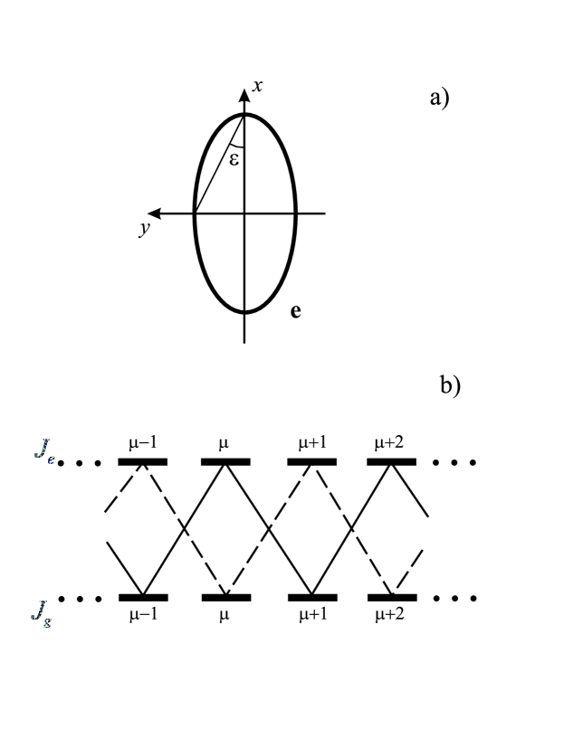
FIG. 1.: Conventional coordinate frame for the representation of elliptical polarization. a) polarization ellipse lies in $xy$-plane, with major axis in $x$-direction. b) transition scheme with the $z$-axis as quantization axis.

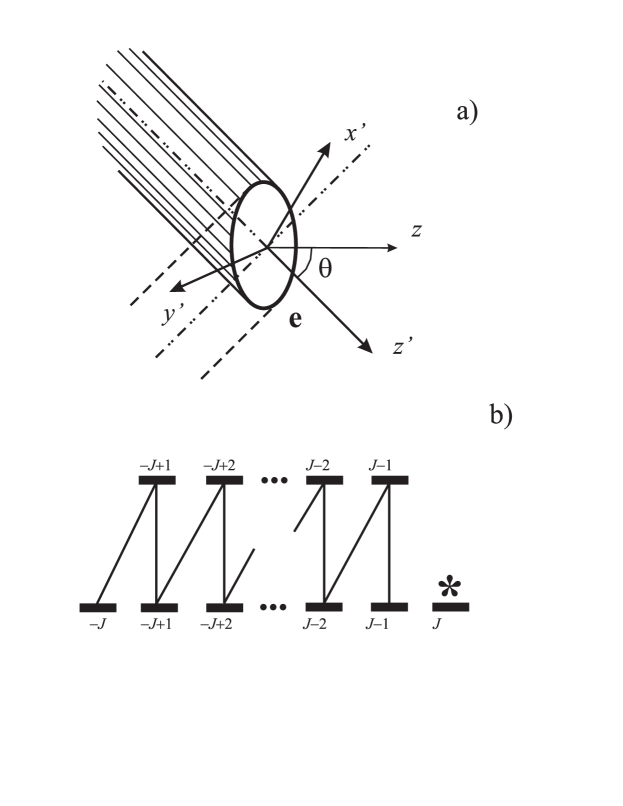
FIG. 2.: Natural coordinate frame for the representation of elliptical polarization. a) polarization vector is superposition of circular polarization defined by cylinder (in $x^{\prime}y^{\prime}$-plane), and linear polarization along axis of cylinder ($z^{\prime}$-axis). b) transition scheme with the $z^{\prime}$-axis as quantization axis.

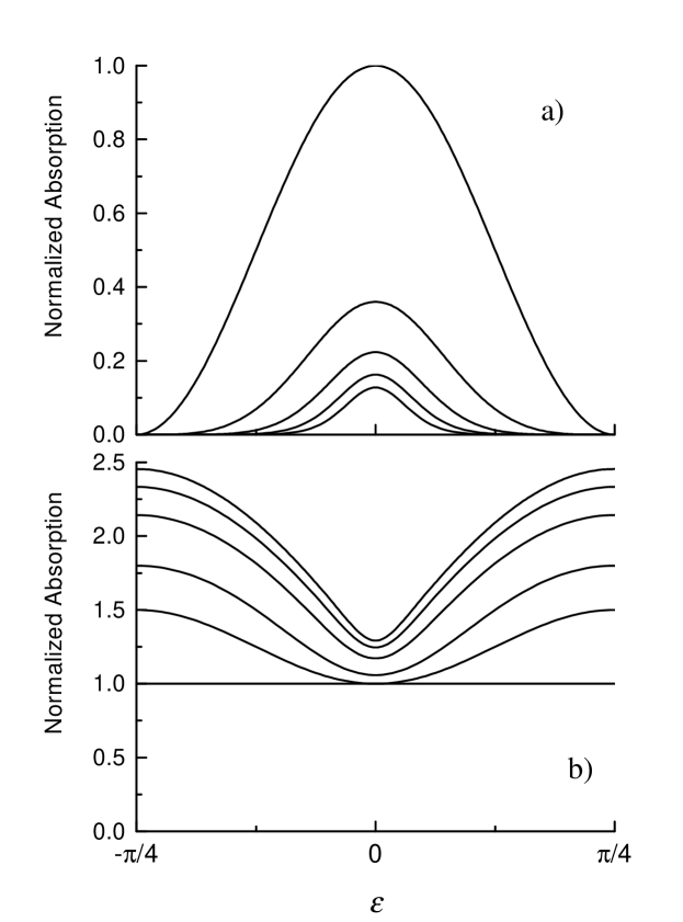
FIG. 3.: Total absorption at low saturation versus the ellipticity $\varepsilon$. (a) transitions $J\to J$ with $J$ a half-integer; $J$ runs from $1/2$ to $9/2$ (from top to bottom). (b) transitions $J\to J+1$; $J=0,\,1/2,\,1,\,2,\,3,\,4$ (from bottom to top). All curves are normalized to the linear absorption.

REFERENCES

• [1] L. Allen and J. H. Eberly Optical Resonance and Two-Level Atoms (John Wiley & Sons, New York-London-Sydney-Toronto, 1975).
• [2] V. S. Letokhov and V. P. Chebotaev, Principles of Nonlinear Laser Spectroscopy, (Springer, Berlin, 1977).
• [3] S. G. Rautian and A. M. Shalagin, Kinetic Problems of Nonlinear Spectroscopy (Elsevier, Amsterdam, 1991).
• [4] V. G. Minogin and V. S. Letokhov, Laser Light Pressure on Atoms (Gordon and Breach, New York, 1987).
• [5] A. P. Kazantsev, G. I. Surdutovich, V. P. Yakovlev, Mechanical Action of Light on Atoms (World Scientific, Singapore, 1990).
• [6] V. S. Smirnov, A. M. Tumaikin, V. I. Yudin, JETP 69, 913 (1989).
• [7] Special Issue Laser Cooling and Trapping of Atoms, J. Opt. Soc. Am. B 6, 11 (1989); Special Issue Laser Cooling and Trapping, Laser Physics 4, 5 (1994); S. Chu, Rev. Mod. Phys. 70, 685 (1998); C. Cohen-Tannoudji, Rev. Mod. Phys. 70, 707 (1998); W. Phillips, Rev. Mod. Phys. 70, 721 (1998).
• [8] E. A. Manykin and V. V. Samartsev, Optical Echo-Spectroscopy [in Russian] (Nauka, Moscow, 1984).
• [9] N. N. Rubtsova, L. S. Vasilenko, E. B. Khvorostov, Laser Physics 9, 239 (1999), and references cited therein.
• [10] A. M. Akulshin, V. L. Velichansky, M. V. Krasheninnikov, V. S. Smirnov, A. M. Tumaikin, V. I. Yudin, Zh. Eksp. Teor. Fiz. 96, 107 (1989) [JETP 69, 58 (1989)].
• [11] J. Dalibard and C. Cohen-Tannoudji, J. Opt. Soc. Amer. B 6, 2023 (1989).
• [12] Y. Castin and K. MΓΈlmer, J. Phys. B 23, 4101 (1990); K. MΓΈlmer, Phys. Rev. A 44, 5820 (1991); J. Javanainen, Phys. Rev. A 44, 5857 (1991); S.M. Yoo and J. Javanainen, Phys. Rev. A 45, 3071 (1992); V. Finkelstein, P.R. Berman, J. Guo, Phys. Rev. A 45, 1829 (1992); J. Werner, H. Wallis, G. Hillenbrand, A. Steane, J. Phys. B 26, 3063 (1993); S. Chang, T. Y. Kwon, H. S. Lee, V. Minogin, Phys. Rev. A 60, 2308 (1999); S. Chang, T. Y. Kwon, H. S. Lee, V.G. Minogin, Phys. Rev. A 64, 013404 (2001).
• [13] P.R. Berman, Phys. Rev. A 43, 1470 (1991); P.R. Berman, G. Rogers, and B. Dubetsky, Phys. Rev. A 48, 1506 (1993).
• [14] G. Nienhuis, P. van der Straten, S.-Q. Shang, Phys. Rev. A 44, 462 (1991).
• [15] J. Macek and I. Hertel, J. Phys. B 7, 2173 (1974).
• [16] G. Nienhuis, Phys. Rev. A 26, 3137 (1982).
• [17] Bo Gao, Phys. Rev. A 48, 2443 (1993).
• [18] J. Dalibard, S. Reynaud and C. Cohen-Tannoudji, J. Phys. B 17, 4577 (1984).
• [19] J. Dalibard and C. Cohen-Tannoudji, J. Opt. Soc. Am. B 6, 2023 (1989).
• [20] D. Suter, Opt. Commun. 86, 381 (1991).
• [21] W. D. Davis, A. L. Gaeta and R. W. Boyd, Optics Lett. 17, 1304 (1992).
• [22] K. MΓΈlmer and C. Westbrook, Laser Physics 4, 872 (1994).
• [23] A. V. Taichenachev, A. M. Tumaikin, V. I. Yudin, G. Nienhuis, Zh. Eksp. Teor. Fiz. 108, 415 (1995) [JETP 81, 224 (1995)].
• [24] A. V. Taichenachev, A. M. Tumaikin, V. I. Yudin, Europhys. Lett. 45, 301 (1999).
• [25] G. Nienhuis, A. V. Taichenachev, A. M. Tumaikin, V. I. Yudin, Europhys. Lett. 44, 20 (1998).
• [26] A.V. Bezverbny, Zh. Eksp. Teor. Fiz. 118, 1066 (2000) [JETP 91, 921 (2000)].
• [27] K.A. Nasyrov, Phys. Rev. A 63, 043406 (2001).
• [28] A. Aspect, E. Arimondo, R. Kaiser, N. Vansteenkiste, and C. Cohen-Tannoudji, Phys. Rev. Lett. 61, 826 (1988); A. Aspect, E. Arimondo, R. Kaiser, N. Vansteenkiste, and C. Cohen-Tannoudji, J. Opt. Soc. Amer. B 6, 2112 (1989).
• [29] F. Mauri and E. Arimondo, Europhys. Lett. 16, 717 (1991).; M. A. Olshanii, J. Phys. B 24, L583 (1991); A.V. Taichenachev, A.M. Tumaikin, V.I. Yudin, M. A. Olshanyi, Pis’ma v Zh. Eksp. Teor. Fiz. 53, 336 (1991) [JETP Lett. 53, 351 (1991)]; F. Mauri and E. Arimondo, Appl. Phys. B 54, 420 (1992); E. Papoff, F. Mauri, E. Arimondo, J. Opt. Soc. Am. B 9, 321 (1992); R. Gupta, S. Padua, C. Xie, H. Batelaan, and H. Metcalf, J. Opt. Soc. Amer. B 11, 537 (1994); G. Morigi, B. Zambon, N. Leinfellner, E. Arimondo, Phys. Rev. A 53, 2616 (1996); C. Menotti, P. Horak, H. Ritsch, J. H. MΓΌller, E. Arimondo, Phys. Rev. A 56, 2123 (1997); C. Menotti, G. Morigi, J. H. MΓΌller, E. Arimondo, Phys. Rev. A 56, 4327 (1997).
• [30] M.A. Olshanii and V.G. Minogin, Opt. Commun. 89, 393 (1992); J. Lawall, F. Bardou, B. Saubamea, K. Shimizu, M. Leduc, A. Aspect, and C. Cohen-Tannoudji, Phys. Rev. Lett.73, 1915 (1994); J. Lawall, S. Kulin, B. Saubamea, N. Bigelow, M. Leduc, C. Cohen-Tannoudji, Phys. Rev. Lett. 75, 4194 (1995).
• [31] A. M. Tumaikin and V. I. Yudin, Zh. Eksp. Teor. Fiz. 98, 81 (1990) [JETP 71, 43 (1990)].
• [32] M. Born and E. Wolf, Principles of Optics (Pergamon, London, 1959).
• [33] G. Nienhuis, Opt. Commun. 59, 353 (1986).
• [34] A. V. Taichenachev, A. M. Tumaikin, V. I. Yudin, G. Nienhuis, Zh. Eksp. Teor. Fiz. 114, 125 (1998) [JETP 87, 70 (1998)].
• [35] D. A. Varshalovich, A. N. Moskalev, V. K. Khersonsky, Quantum Theory of Angular Momentum (World Scientific, Singapore, 1988).
• [36] N. L. Manakov, S. I. Marmo, and A. V. Meremianin, J. Phys. B: At. Mol. Opt. Phys. 29, 2711, (1996).
• [37] N. L. Manakov and A. V. Merem’yanin, Zh. Eksp. Teor. Fiz. 111, 1984 (1997) [JETP 84, 1080 (1997)].
• [38] N. Ya. Vilenkin, Special Functions and the Theory of Group Representations (American Mathematical Society, Providence, 1968).
• [39] F. R. Gantmacher, The Theory of Matrices (Chelsea, New York, 1959).
• [40] U. Fano and G. Racah, Irreducible Tensorial Sets (Academic, New York, 1959).
• [41] A. V. Taichenachev, A. M. Tumaikin, V. I. Yudin, Zh. Eksp. Teor. Fiz. 110, 1727 (1996) [JETP 83, 949 (1996)].
• [42] A. V. Taichenachev, A. M. Tumaikin, V. I. Yudin, Zh. Eksp. Teor. Fiz. 118, 77 (2000). [JETP 91, 67 (2000)].
• [43] A. V. Taichenachev, A. M. Tumaikin, V. I. Yudin, Pis’ma v Zh. Eksp. Teor. Fiz. 64, 8 (1996) [JETP Lett. 64, 7 (1996)].
• [44] A. M. Akulshin, S. Barreiro, A. Lezama, Phys. Rev. A 57, 2996 (1998); A. Lezama, S. Barreiro, A. M. Akulshin, Phys. Rev. A 59, 4732 (1999); A. V. Taichenachev, A. M. Tumaikin, V. I. Yudin, Phys. Rev. A 61, 011802 (2000); Y. Dancheva, G. Alzetta, S. Cartaleva, M. Taslakov, Ch. Andreva, Optics Comm. 178, 103 (2000); F. Renzoni, S. Cartaleva, G. Alzetta, E. Arimondo, Phys. Rev. A 63, 065401 (2001); A. V. Papoyan, M. Auzinsh, K. Bergmann, Eur. Phys. J. D 21, 63 (2002); C. Goren, A. D. Wilson-Gordon, M. Rosenbluh, H. Friedmann, Phys. Rev. A 67, 033807 (2003); H. Failache, P. Valente, G. Ban, V. Lorent, A. Lezama, Phys. Rev. A 67, 043810 (2003).
• [45] H.F. Arnoldus and G. Nienhuis, J. Phys. B: At. Mol. Phys. 16, 2325 (1983).
• [46] A. V. Bezverbnyi, A. M. Tumaikin, G. Nienhuis, Opt. Commun. 148, 151 (1998).
• [47] A. V. Taichenachev, A. M. Tumaikin, V. I. Yudin, Laser Physics 2, 575 (1992); R. Dum and M. Olshanii, Phys. Rev. Lett. 76, 1788 (1996); P. M. Visser and G. Nienhuis, Phys. Rev. A 57, 4581 (1998).
Refer to caption