On duality between quantum maps and quantum states

Abstract

We investigate the space of quantum operations, as well as the larger space of maps which are positive, but not completely positive. A constructive criterion for decomposability is presented. A certain class of unistochastic operations, determined by unitary matrices of extended dimensionality, is defined and analyzed. Using the concept of the dynamical matrix and the Jamiołkowski isomorphism we explore the relation between the set of quantum operations (dynamics) and the set of density matrices acting on an extended Hilbert space (kinematics). An analogous relation is established between the classical maps and an extended space of the discrete probability distributions.

e-mail: karol@cft.edu.pl   ingemar@physto.se

I Introduction

The theory of quantum information has been studied for at least forty years – consult e.g. some early papers by Ingarden and his group written in sixties and seventies IU62 ; IK68 ; Ko69 ; In75 . However, rapid progress of this theory occurred only in the last decade Gr99 ; BEZ00 ; NC00 ; ABHH+01 ; Ke02 , due to a synergetic feedback with several recent experiments on quantum physics, motivated by information encoding and processing. The possibility to encode the information in quantum states triggered an increasing interest in the structure and the properties of the set of quantum states MaW95 ; AMM97 ; JS01 ; Ki03 ; BK03 . Usually one considers states acting on a finite dimensional Hilbert space, ${\cal H}_{N}$.

To characterize the way that information is processed according to the laws of quantum mechanics, one needs to describe the dynamics of the density matrices. In many cases it is sufficient to consider discrete dynamics, which maps an initial state $\rho$ into the final state $\rho^{\prime}$. Such maps are often called quantum channels, and their theory is a subject of considerable recent interest OP93 ; IKO97 ; AF01 ; BP02 .

The set of quantum states ${\cal M}^{(N)}$ consists of density matrices of size $N$, which are normalized, hermitian, and positive definite. A quantum channel is called positive, if it maps the set of positive operators into itself. However, since a physical system under consideration may be coupled with an environment, the maps describing physical processes should be completely positive (CP), which means that all their extensions into higher dimensional spaces remain positive. Any CP map may be (not uniquely) represented in the so–called Kraus form, by a collection of Kraus operators Kr83 .

Even though positive, but not completely positive, maps cannot be realized in the laboratory, they are of a great theoretical importance, since they can be used to detect entanglement in density matrices written on paper HHH96a ; Ho01 . The phenomenon of quantum entanglement seems to be crucial in the theory of quantum information. The structure of the set of all completely positive maps, ${\cal CP}_{N}$, is relatively well understood Cho75a , but the task to characterize the larger set of all positive maps is far from being completed TT83 ; Ky96 ; MM01 .

The aim of this work is twofold. On one hand we present a concise review of recent development concerning the properties of the set of quantum maps. On the other hand, we present several new results in this field. In particular, in section 2 concerning the matrix algebra, we define a simple transformation of a matrix, called reshuffling, and establish a useful lemma: The Schmidt coefficients of a matrix $A$, treated as an element of a composite Hilbert-Schmidt space of operators, are equal to the squared singular values of the reshuffled matrix $A^{R}$. In section 3 we investigate the properties of the dynamical matrix $D$ associated with any linear map SMR61 - it may be obtained by reshuffling of the superoperator $L$ which describes the map. Furthermore, we define a class of unistochastic maps, which are determined by a single unitary matrix $U$ of size $N^{2}$.

For any CP map the corresponding dynamical matrix $D$ is hermitian and positive definite. Making use of the eigen representation of $D$ one may define the canonical Kraus form of the operation. In section 5 we present a comparison between different classes of quantum maps, acting on the space of density matrices, with the classes of classical maps acting on the simplex $\Delta_{N-1}$ of discrete, $N$–point probability measures. For concreteness we present in section 6 certain exemplary maps acting in the space of qubits - the density matrices of size $N=2$.

In section 7 the positive, co-positive and decomposable maps are analyzed and a constructive criterion for decomposability of a map is provided. Furthermore, for any quantum map we introduce three quantities useful to locate it with respect to the boundaries of the sets of positive (CP, CcP) maps. In the subsequent sections we explore the Jamiołkowski isomorphism Ja72 , which relates the set of quantum maps acting on ${\cal M}^{(N)}$, with the states from ${\cal M}^{(N^{2})}$, which act on the extended Hilbert space ${\cal H}_{N}\otimes{\cal H}_{N}$. This isomorphism, formulated as well in the quantum, as well as in the classical setup, allows us to discover an analogy between objects, sets and problems concerning quantum maps and quantum states. This key issue of the work explains its title: there exists a kind of duality between between properties of the set of quantum maps (dynamics) and the the set quantum states of a composite $N\times N$ system (kinematics).

II Algebraic detour: matrix reshaping and reshuffling

In this section we are going to discuss some simple algebraic transformations performed on complex matrices, which prove useful in description of quantum maps. In particular, we introduce a convenient notation to work in the composite Hilbert space ${\cal H}_{N}\otimes{\cal H}_{M}$ or in the Hilbert–Schmidt (HS) space of linear operators, ${\cal H}_{\rm HS}$.

Consider a rectangular matrix $A_{ij}$, $i=1,...,M$ and $j=1,...,N$. The matrix may be reshaped, by putting its elements row after row in lexicographical order into a vector $\vec{a}_{k}$ of size $MN$,

$${\vec{a}}_{k}=A_{ij}\quad{\rm where}\quad k=(i-1)N+j,\quad i=1,...,M,\quad j=1,...N.$$ (1)

Conversely, any vector of length $MN$ may be reshaped into a rectangular matrix. The simplest example of such a vectorial notation of matrices reads

$$A\ =\ \left[\begin{array}[]{cc}A_{11}&A_{12}\\ A_{21}&A_{22}\end{array}\right]\quad\longleftrightarrow\quad{\vec{a}}\ =\ \{A_{11},A_{12},A_{21},A_{22}\}.$$ (2)

The scalar product between any two elements of the HS space ${\cal H}_{\rm HS}$ (matrices of size $N$) may be rewritten as an ordinary scalar product between two corresponding vectors of size $N^{2}$,

$$\langle A|B\rangle\equiv{\rm Tr}A^{\dagger}B={\vec{a}}^{*}\cdot{\vec{b}}=\langle a|b\rangle.$$ (3)

Thus the HS norm of a matrix is equal to the norm of the associated vector, $||A||^{2}_{HS}=|{\vec{a}}|^{2}$.

Sometimes we will use both indices and label a component of ${\vec{a}}$ by $a_{ij}$. This vector of length $MN$ may be linearly transformed into $a^{\prime}=Ca$ by a matrix $C$ of size $MN\times MN$. Its elements may be denoted by $C_{kk^{\prime}}$ with $k,k^{\prime}=1,...,MN$, but it is also convenient to use a four index notation, $C_{\stackrel{{\scriptstyle\scriptstyle m\mu}}{{n\nu}}}$ where $m,n=1,...,N$ while $\mu,\nu=1,...,M$. In this notation the elements of the transposed matrix are $C_{\stackrel{{\scriptstyle\scriptstyle m\mu}}{{n\nu}}}^{T}=C_{\stackrel{{\scriptstyle\scriptstyle n\nu}}{{m\mu}}}$, since the upper pair of indices determines the row of the matrix $C$, while the lower pair determines its column. The matrix $C$ may represent an operator acting in a composite space ${\cal H}={\cal H}_{N}\otimes{\cal H}_{M}$. The tensor product of any two bases in both subspaces provides a basis in ${\cal H}$, so that

$$C_{\stackrel{{\scriptstyle\scriptstyle m\mu}}{{n\nu}}}=\langle e_{m}\otimes f_{\mu}|C|e_{n}\otimes f_{\nu}\rangle,$$ (4)

where the Roman indices refer to variables of the first subsystem, ${\cal H}_{A}={\cal H}_{N}$, and the Greek indices to the second, ${\cal H}_{B}={\cal H}_{M}$. The trace of a matrix reads Tr$C=C_{\stackrel{{\scriptstyle\scriptstyle m\mu}}{{m\mu}}}$, where summation over the repeating indices is assumed. The operation of partial trace over the second subsystem produces the matrix $C^{A}\equiv{\rm Tr}_{B}C$ of size $N$, while tracing over the first subsystem leads to a $M\times M$ matrix $C^{B}\equiv{\rm Tr}_{A}C$,

$$C^{A}_{mn}=C_{\stackrel{{\scriptstyle\scriptstyle m\mu}}{{n\mu}}},{\rm\quad\quad and\quad\quad}C^{B}_{\mu\nu}=C_{\stackrel{{\scriptstyle\scriptstyle m\mu}}{{m\nu}}}.$$ (5)

If $C$ is a tensor product, $C=A\otimes B$, then $C_{\stackrel{{\scriptstyle\scriptstyle m\mu}}{{n\nu}}}=A_{mn}B_{\mu\nu}$.

Consider a unitary matrix $\tilde{U}$ of size $N^{2}$. Its $N^{2}$ columns (rows) ${\vec{\tilde{u}}}_{k},k=1,...,N^{2}$ reshaped into square matrices ${\tilde{U}}_{k}$ of size $N$ form an orthogonal basis in ${\cal H}_{HS}$. Using the Hilbert-Schmidt norm, $||A||_{HS}=({\rm Tr}AA^{\dagger})^{1/2}$, we normalize them according to $A_{k}={\tilde{U}}_{k}/||\tilde{U}_{k}||_{HS}$ and obtain the orthonormal basis, $\langle A_{k}|A_{j}\rangle\equiv{\rm Tr}A_{k}^{\dagger}A_{j}=\delta_{kj}$. Alternatively, in a double index notation with $k=(m-1)N+\mu$ and $j=(n-1)N+\nu$ this orthogonality relation reads $\langle A^{m\mu}|A^{n\nu}\rangle=\delta_{mn}\delta_{\mu\nu}$. Note that in general the matrices $A_{k}$ (also denoted by $A^{m\mu}$) are not unitary.

Let $X$ denote an arbitrary matrix of size $N^{2}$. It may be represented as a double (quadruple) sum,

$$|X\rangle=\sum_{k=1}^{N^{2}}\sum_{j=1}^{N^{2}}C_{kj}|A_{k}\rangle\otimes|A_{j}\rangle=C_{\stackrel{{\scriptstyle\scriptstyle m\mu}}{{n\nu}}}|A^{m\mu}\rangle\otimes|A^{n\nu}\rangle$$ (6)

where $C_{kj}={\rm Tr}((A_{k}\otimes A_{j})^{\dagger}X)$ may be neither Hermitian nor normal (which means that $C$ and $C^{\dagger}$ need not commute). The matrix $X$ may be considered as a vector in the composite Hilbert-Schmidt space, ${\cal H}_{\rm HS}\otimes{\cal H}_{\rm HS}$, so applying its Schmidt decomposition Pe95b we arrive at

$$|X\rangle=\sum_{k=1}^{N^{2}}{\sqrt{\lambda_{k}}}|A_{k}^{\prime}\rangle\otimes|A_{k}^{\prime\prime}\rangle,$$ (7)

where $\sqrt{\lambda_{k}}$ are the singular values of $C$, i.e. the square roots of the non-negative eigenvalues of $CC^{\dagger}$. The sum of their squares is determined by the norm of the operator, $\sum_{k=1}^{N^{2}}\lambda_{k}={\rm Tr}(XX^{\dagger})=||X||_{HS}^{2}$.

Since the Schmidt coefficients do not depend on the initial basis let us analyze the special case, in which the basis in ${\cal H}_{HS}$ is generated by the identity matrix, $U={\mathbbm{1}}$ of size $N^{2}$. Then each of the $N^{2}$ basis matrices of size $N$ consist of only one non-zero element which equals unity, $A_{k}=A^{m\mu}=|m\rangle\langle\mu|$, where $k=N(m-1)+\mu$. Their tensor products form an orthonormal basis in ${\cal H}_{HS}\otimes{\cal H}_{HS}$ and allow to represent an arbitrary matrix $X$ in the form (6). In this case the matrix of the coefficients $C$ has a particularly simple form, $C_{\stackrel{{\scriptstyle\scriptstyle m\mu}}{{n\nu}}}={\rm Tr}[(A^{m\mu}\otimes A^{n\nu})X]=X_{\stackrel{{\scriptstyle\scriptstyle mn}}{{\mu\nu}}}$.

This particular reordering of a matrix deserves a name so we shall write $X^{R}\equiv C(X)$ defining the following procedure of reshuffling of matrices. Using this notion our findings may be summarized in the following lemma:

Schmidt coefficients of an operator $X$ acting on a bi-partite Hilbert space are equal to the squared singular values of the reshuffled matrix, $X^{R}$.

More precisely, the Schmidt decomposition (7) of any operator $X$ of size $MN$ may be supplemented by a set of three equations

$$\left\{\begin{array}[]{ccc}\{\lambda_{k}\}_{k=1}^{N^{2}}&=&\bigl{\{}{\rm SV}(X^{R})\bigr{\}}^{2}\ \ :\ \ {\rm\ \ eigenvalues\ \ of\ \ }(X^{R})^{\dagger}X^{R}\\ |A^{\prime}\rangle&\ :&{\rm\ \ reshaped\ \ eigenvectors\ \ of\ \ }(X^{R})^{\dagger}X^{R}\\ |A^{\prime\prime}\rangle&\ :&{\rm\ \ reshaped\ \ eigenvectors\ \ of\ \ }X^{R}(X^{R})^{\dagger}\\ \end{array}\right.,$$ (8)

where we have assumed that $N\leq M$. The initial basis is transformed by a local unitary transformation $W_{a}\otimes W_{b}$, where $W_{a}$ and $W_{b}$ are matrices of eigenvectors of matrices $(X^{R})^{\dagger}X^{R}$ and $X^{R}(X^{R})^{\dagger}$, respectively. Iff rank $r$ of $X^{R}(X^{R})^{\dagger}$ equals one, the operator can be factorized into a product form, $X=X_{1}\otimes X_{2}$, where $X_{1}={\rm Tr}_{2}X$ and $X_{2}={\rm Tr}_{1}X$.

Table 1: Reorderings of a matrix $X$ representing an operator which acts on a composed Hilbert space. The arrows denote the indices exchanged.

Transformation	definition	symbol	preserves Hermicity	preserves spectrum
transposition	$X_{\stackrel{{\scriptstyle\scriptstyle m\mu}}{{n\nu}}}^{T}=X_{\stackrel{{\scriptstyle\scriptstyle n\nu}}{{m\mu}}}$	$\updownarrow\updownarrow$	yes	yes
flip	$X_{\stackrel{{\scriptstyle\scriptstyle m\mu}}{{n\nu}}}^{F}=X_{\stackrel{{\scriptstyle\scriptstyle\mu m}}{{\nu n}}}$	${\stackrel{{\scriptstyle\textstyle\leftrightarrow}}{{\leftrightarrow}}}$	yes	yes
partial	$X_{\stackrel{{\scriptstyle\scriptstyle m\mu}}{{n\nu}}}^{T_{A}}=X_{\stackrel{{\scriptstyle\scriptstyle n\mu}}{{m\nu}}}$	$\updownarrow.$	yes	no
transpositions	$X_{\stackrel{{\scriptstyle\scriptstyle m\mu}}{{n\nu}}}^{T_{B}}=X_{\stackrel{{\scriptstyle\scriptstyle m\nu}}{{n\mu}}}$	$.\updownarrow$	yes	no
reshuffling	$X_{\stackrel{{\scriptstyle\scriptstyle m\mu}}{{n\nu}}}^{R}=X_{\stackrel{{\scriptstyle\scriptstyle mn}}{{\mu\nu}}}$	$\nearrow\!\!\!\!\!\!\swarrow$	no	no
reshuffling ′	$X_{\stackrel{{\scriptstyle\scriptstyle m\mu}}{{n\nu}}}^{R^{\prime}}=X_{\stackrel{{\scriptstyle\scriptstyle\nu\mu}}{{nm}}}$	$\nwarrow\!\!\!\!\!\!\searrow$	no	no
partial	$X_{\stackrel{{\scriptstyle\scriptstyle m\mu}}{{n\nu}}}^{F_{1}}=X_{\stackrel{{\scriptstyle\scriptstyle\mu m}}{{n\nu}}}$	${\stackrel{{\scriptstyle\textstyle\leftrightarrow}}{{.}}}$	no	no
flips	$X_{\stackrel{{\scriptstyle\scriptstyle m\mu}}{{n\nu}}}^{F_{2}}=X_{\stackrel{{\scriptstyle\scriptstyle m\mu}}{{\nu n}}}$	${\stackrel{{\scriptstyle\textstyle.}}{{\leftrightarrow}}}$	no	no

In general, one may reshuffle square matrices, if its size $K$ is not prime. The symbol $X^{R}$ has a unique meaning if a concrete decomposition of the size $K=MN$ is specified. If $M\neq N$ the matrix $X^{R}$ is a $N^{2}\times M^{2}$ rectangular matrix. Since $(X^{R})^{R}=X$ we see that one may also reshuffle rectangular matrices, provided both dimensions are squares of natural numbers. Similar reorderings of matrices were considered by Hill et al. OH85 ; YH00 while investigating CP maps and later in Rud02 ; HHH02 ; CW03 ; Rud03 ; ACF03 to analyze separability of mixed quantum states.

To get a better feeling of the reshuffling transformation observe that reshaping each row of an initially square matrix $X$ of size $MN$ according to Eq. (1) into a rectangular $M\times N$ submatrix, and placing it according to the lexicographical order block after block, one produces the reshuffled matrix $X^{R}$. Let us illustrate this procedure for the simplest case $N=M=2$, in which any row of the matrix $X$ is reshaped into a $2\times 2$ matrix

$$C_{kj}=X_{kj}^{R}\equiv\left[\begin{array}[]{c|c}{\bf{X_{11}\ \ X_{12}}}&X_{21}{\rm~{}~{}~{}}X_{22}\\ X_{13}{\rm~{}~{}~{}}X_{14}&{\bf X_{23}\ \ X_{24}}\\ \hline\cr{\bf X_{31}\ \ X_{32}}&X_{41}{\rm~{}~{}~{}}X_{42}\\ X_{33}{\rm~{}~{}~{}}X_{34}&{\bf X_{43}\ \ X_{44}}\end{array}\right].$$ (9)

The operation of reshuffling could be defined in an alternative way, say the reshaping of the matrix $A$ from (1) could be performed column after column into a vector ${\vec{a}}^{\prime}$. In the four indices notation introduced above (Roman indices running from $1$ to $N$ correspond to the first subsystem, Greek indices to the second one), both operations of reshuffling take the form

$$X_{\stackrel{{\scriptstyle\scriptstyle m\mu}}{{n\nu}}}^{R}\equiv X_{\stackrel{{\scriptstyle\scriptstyle mn}}{{\mu\nu}}}{\quad\quad\quad\rm and\quad\quad\quad}X_{\stackrel{{\scriptstyle\scriptstyle m\mu}}{{n\nu}}}^{R^{\prime}}\equiv X_{\stackrel{{\scriptstyle\scriptstyle\nu\mu}}{{nm}}}.$$ (10)

However, both reshuffled matrices are equivalent up to a certain permutation of rows and columns and transposition, so the singular values of $X^{R^{\prime}}$ and $X^{R}$ are equal. It is easy to see that $(X^{R})^{R}=X.$ In the symmetric case with $M=N$, $N^{3}$ elements of $X$ do not change their position during the operation of reshuffling (these are typeset boldface in (9)); while the other $N^{4}-N^{3}$ elements are exchanged. The space of complex matrices with the reshuffling symmetry, $X=X^{R}$, is thus $2N^{4}-2(N^{4}-N^{3})=2N^{3}$ dimensional.

For comparison we provide analogous formulae showing the action of partial transposition: with respect to the first subsystem, $T_{A}\equiv T\otimes{\mathbbm{1}}$ and with respect to the second, $T_{B}\equiv{\mathbbm{1}}\otimes T$,

$$X_{\stackrel{{\scriptstyle\scriptstyle m\mu}}{{n\nu}}}^{T_{A}}=X_{\stackrel{{\scriptstyle\scriptstyle n\mu}}{{m\nu}}}{\quad\quad\rm and\quad\quad}X_{\stackrel{{\scriptstyle\scriptstyle m\mu}}{{n\nu}}}^{T_{B}}=X_{\stackrel{{\scriptstyle\scriptstyle m\nu}}{{n\mu}}}.$$ (11)

Note that all these operations consist of exchanging a given pair of indices. However, while partial transposition (11) preserves Hermicity, the reshuffling (10) does not. For convenience we shall define a related transformation of flip among both subsystems, $X_{\stackrel{{\scriptstyle\scriptstyle m\mu}}{{n\nu}}}^{F}\equiv X_{\stackrel{{\scriptstyle\scriptstyle\mu m}}{{\nu n}}}$, the action of which consists in relabeling of certain rows (and columns) of the matrix, so its spectrum remains preserved. Note that for a tensor product $X=Y\otimes Z$ one has $X^{F}=Z\otimes Y$. In full analogy to partial transposition we use also two operations of partial flip (see table 1). All the above transformations are involutions, since performed twice they are equal to identity. It is not difficult to find relations between them, e.g. $X^{F_{1}}=[(X^{R^{\prime}})^{T_{A}}]^{R^{\prime}}=[(X^{R})^{T_{B}}]^{R}$. Since $X^{R^{\prime}}=[(X^{R})^{F}]^{T}=[(X^{R})^{T}]^{F}$, while $X^{T_{B}}=(X^{T_{A}})^{T}$ and $X^{F_{1}}=(X^{F_{2}})^{F}$, thus the spectra and singular values of the reshuffled (partially transposed, partially flipped) matrices do not depend on the way, each operation has been performed, i.e. eig$(X^{R})={\rm eig}(X^{R^{\prime}})$ and SV$(X^{R})={\rm SV}(X^{R^{\prime}})$, (eig$(X^{F_{1}})={\rm eig}(X^{F_{2}})$ and SV$(X^{F_{1}})={\rm SV}(X^{F_{2}})$).

III Completely positive maps

Let $\rho\in{\cal M}^{(N)}$ be a density operator acting on a $N$-dimensional Hilbert space ${\cal H}_{N}$. What conditions need to be fulfilled by a map $\Phi:{\cal M}^{(N)}\to{\cal M}^{(N)}$, so it could represent a physical operation? If the map is linear than the image of a mixed state $\rho$ does not depend on the way, how the state $\rho$ was constructed out of projectors. This is a very important feature, since it allows for a probabilistic interpretation of any mixed state. Furthermore, we assume that the map is trace preserving, Tr$\rho={\rm Tr}\Phi(\rho)$, which corresponds to the conservation of probability.

Any quantum operation has to be positive – it should map any positive density operator into a positive operator. Strictly speaking the term ’positive’ refers to positive semidefinite Hermitian operators, which do not have negative eigenvalues. However, this condition occurs not to be sufficient to produce physically realizable transformations. Any quantum state $\rho$ may be extended by an ancilla $\sigma$ into a tensor product acting in a $KN$ dimensional Hilbert space. Hence the evolution of a linear map $\Phi$ may be considered as the evolution of a part $\rho$ of a larger system $\rho\otimes\sigma$. Therefore we should require complete positivity St55 ; Ar69 , which means that for an arbitrary $K$ dimensional extension

$${\cal H}_{N}\to{\cal H}_{N}\otimes{\cal H}_{K}\quad{\rm the\quad map}\quad\Phi\otimes{\mathbbm{1}}_{K}\quad{\rm is\quad positive}.$$ (12)

If the above requirement holds for any fixed $K$, such a property is called $K$–positivity St55 ; Da76 ; Kr83 . Constructing the dynamical matrix we will show in the next section that any $N$–positive map $\Phi$ acting on ${\cal M}^{(N)}$ is completely positive Cho72 . The importance of complete positivity in quantum mechanics was emphasized in the seventies by Kraus Kr71 , Lindblad Li76 and Accardi Ac76 , and the restriction to CP maps is not trivial: There exist quantum maps which are positive but not completely positive St55 . A simple and important example consists of transposition $T$ of an operator in a given basis Per96 , which for Hermitian operators is equivalent to complex conjugation: if $A=A^{\dagger}$ then $A^{T}={\bar{A}}$. Although the map $T(\rho)=\rho^{T}$ preserves the spectrum and therefore is positive, its extension $T_{A}\equiv T\otimes{\mathbbm{1}}$, called partial transposition, is not, as discussed in section VII.

A linear CP-map which preserves the trace is called a quantum operation or quantum channel. Any linear, completely positive map $\Phi$ may be represented Kr71 ; Kr83 by a collection of $k$ Kraus operators $A_{i}$ in the so–called Kraus form

$$\rho\to\rho^{\prime}={\Phi}(\rho)=\sum_{i=1}^{k}A_{i}\rho A_{i}^{\dagger}.$$ (13)

It is also called an operator sum representation of the map $\Phi$ or the Stinespring form, since its existence follows from the Stinespring dilation theorem St55 ; Ev84 . If the set of Kraus operators satisfies the completeness relation

$$\sum_{i=1}^{k}A_{i}^{\dagger}A_{i}={\mathbbm{1}},$$ (14)

the map is trace preserving: for any initial state $\rho$ one has ${\rm Tr}\bigl{(}\sum_{i=1}^{k}A_{i}^{\dagger}A_{i}\rho\bigr{)}=$ ${\rm Tr}\bigl{[}{\Phi(\rho)}\bigr{]}={\rm Tr}\rho=1$. Thus, the Kraus operators may be considered as measurement operators while any trace preserving CP map may be interpreted as a generalized measurement Pe95b .

Let us denote the elements of the Kraus operators $A_{i}$ represented in an orthonormal basis by $A^{(i)}_{mn}$. Define a Kraus matrix $M$ of size $N$ composed of non-negative entries St02 ,

$$M_{mn}=\sum_{i=1}^{k}|A_{mn}^{(i)}|^{2},$$ (15)

where the Kraus operators are now denoted by $A^{(i)}$. The completeness relation (14) enforces that the sum of elements in each column of $M$ equals to unity, so it is a stochastic matrix. Thus quantum operations are often called stochastic maps.

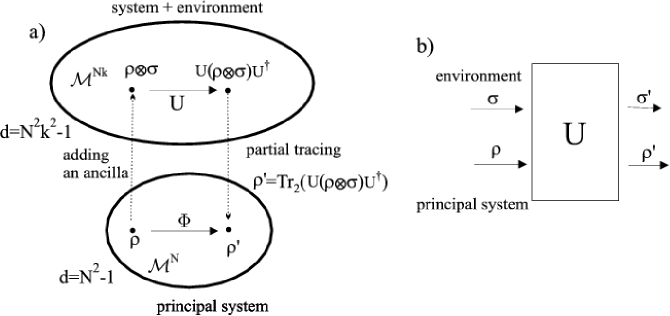
Figure 1: Quantum operations represented by a) unitary operator $U$ of size $NK$ in an enlarged system including the environment, b) black box picture, in which $U$ couples the principal $N$–dimensional system $\rho$ with the environment $\sigma$ of dimensionality $K$.

Any map written in the Kraus form (13) is linear and preserves the trace if the condition (14) is fulfilled. Let $\rho$ denote the density operator of the investigated quantum system. The time evolution of an isolated quantum system is unitary, while all sorts of a non unitary dynamics reflect its interaction with an environment, described by a density operator $\sigma$. However, if we extend the system and study the dynamics of the total system, $\rho\otimes\sigma$, composed of the system under investigation and the environment, its time evolution remains unitary Ar69 ; EL77 . The non unitary operation of $\rho$ emerges as an effect of the partial tracing with respect to the environment,

$$\rho\to\rho^{\prime}={\Phi}(\rho)={\rm Tr}_{\rm env}\Bigl{[}U\bigl{(}\rho\otimes\sigma\bigr{)}U^{\dagger}\Bigr{]}.$$ (16)

The above form is called as environmental representation of the map $\Phi$. The entire process may be considered as a composition of three basic steps: adding an ancilla, unitary transformation, and partial tracing. The forms (13) and (16) are equivalent in the sense that any quantum operation may be written either way. Both representations are not unique, but as discussed in section IV, the notion of a dynamical matrix allows one to define a distinguished, canonical Kraus form.

Let the principal $N$–dimensional system $\rho$ be subjected to an operation defined by the $kN$ dimensional matrix $U$ and an initially pure state of the environment $\sigma=|\nu\rangle\langle\nu|$,

$$\rho^{\prime}={\Phi}(\rho)={\rm Tr}_{\rm env}\Bigl{[}U\bigr{(}\rho\otimes|\nu\rangle\langle\nu|\bigl{)}U^{\dagger}\Bigr{]}=\sum_{\mu=1}^{k}\langle\mu|U|\nu\rangle\rho\langle\nu|U^{\dagger}|\mu\rangle.$$ (17)

Since the fixed environmental state $|\nu\rangle$ belongs to the $k$-dimensional Hilbert space ${\cal H}_{\rm env}$, the expression $\langle\mu|U|\nu\rangle$ represents a square matrix of size $N$, which we shall call $A_{\mu}$. In the double index notation, introduced above, any element of the unitary matrix is denoted by $U_{\stackrel{{\scriptstyle\scriptstyle m\mu}}{{n\nu}}}$, while the matrix $A_{\mu}=\langle\mu|U|\nu\rangle$ consists of elements

$$A^{(\mu)}_{mn}=\langle m,\mu|U|n,\nu\rangle=U_{\stackrel{{\scriptstyle\scriptstyle m\mu}}{{n\nu}}}.$$ (18)

It is easy to see that (17) takes the operator sum form, $\sum_{\mu=1}^{k}A_{\mu}\rho A_{\mu}^{\dagger}$. Moreover, due to unitarity of $U$ the operators $A_{\mu}$ satisfy the completeness relation

$$\sum_{\mu=1}^{k}A_{\mu}^{\dagger}A_{\mu}=\sum_{\mu=1}^{k}\langle\nu|U^{\dagger}|\mu\rangle\langle\mu|U|\nu\rangle=\langle\nu|U^{\dagger}U|\nu\rangle={\mathbbm{1}}_{N}$$ (19)

and may be considered as Kraus operators. Every element of a given matrix $A_{\mu}$ belongs to one of the $N^{2}$ blocks of size $k$ of the unitary matrix $U$. However, if we reorder it constructing $U_{\stackrel{{\scriptstyle\scriptstyle m\mu}}{{n\nu}}}^{F}=U_{\stackrel{{\scriptstyle\scriptstyle\mu m}}{{\nu n}}}$, then each matrix $A_{\mu}$ is just a truncation of the flipped matrix $U^{F}$, since $A^{(\mu)}_{mn}=U_{\stackrel{{\scriptstyle\scriptstyle\mu m}}{{\nu n}}}^{F}$ represents its minor.

If the initial state of the environment in the representation (16) is chosen to have full rank, $\sigma=\sum_{\nu=1}^{k}q_{\nu}|\nu\rangle\langle\nu|$, the operator sum representation consists of $kN$ terms

$$\rho^{\prime}={\Phi}(\rho)={\rm Tr}_{\rm env}\Bigl{[}U\Bigr{(}\rho\otimes\sum_{\nu=1}^{k}q_{\nu}|\nu\rangle\langle\nu|\Bigl{)}U^{\dagger}\Bigr{]}=\sum_{l=1}^{kN}A_{l}\rho A_{l}^{\dagger}$$ (20)

where $A_{l}=\sqrt{q_{\mu}}\langle\mu|U|\nu\rangle$ and $l=\mu+\nu(k-1)$.

In this way we have shown that for any operation written in the environmental form (16) we may find a corresponding Kraus form. Conversely, for any quantum operation in the Kraus form (13) consisting of $k$ operators we may construct an environmental form Ar69 ; Li75 . For instance take the first $N$ columns of a unitary matrix $U$ of size $kN$ are constructed of $k$ Kraus operators as defined in (18). Due to the completeness relation (14) they are normalized and orthogonal. The matrix $U$ has to be completed by $N(k-1)$ complex orthogonal vectors; they do not influence the quantum operation and may be selected arbitrarily.

If the initial state of the environment is pure its dimensionality $k$ of ${\cal H}_{\rm env}$ needs not to exceed $N^{2}$, the maximal number of Kraus operators required. If the environment is initially in a mixed state, its weights coefficients $q_{j}$ are needed to specify the operation. Counting the number of parameters one could thus speculate that the action of any quantum operation may be simulated by a coupling with a mixed state of the environment of size $N$. However, this is not the case: already for $N=2$ there exist operations which have to be simulated with $3$–dimensional environment TCDGS99 ; ZR02 , and the general question of the minimal size of ${\cal H}_{\rm env}$ remains open.

It is also illuminating to discuss a special case of the problem, in which the initial state of the $N$–dimensional environment is maximally mixed, $\sigma=\rho_{*}={\mathbbm{1}}_{N}/N$. The unitary matrix $U$ of size $N^{2}$, defining the map, may be treated as a vector in the composed Hilbert–Schmidt space ${\cal H}_{\rm HS}\otimes{\cal H}_{\rm HS}$ and represented in its Schmidt form (7), $U=\sum_{i=1}^{N^{2}}\sqrt{\lambda_{i}}|{\tilde{A}}_{i}\rangle\otimes|{\tilde{A}}_{i}^{\prime}\rangle$, where $\lambda_{i}$ are eigenvalues of $(U^{R})^{\dagger}U^{R}$. Since the operators ${\tilde{A}}_{i}^{\prime}$, obtained by reshaping eigenvectors of $(U^{R})^{\dagger}U^{R}$, form an orthonormal basis in ${\cal H}_{\rm HS}$, the procedure of partial tracing leads to the Kraus form consisting of $N^{2}$ terms:

$$\rho^{\prime} ={\Phi}_{U}(\rho)={\rm Tr}_{\rm env}\Bigl{[}U(\rho\otimes\frac{1}{N}{\mathbbm{1}}_{N})U^{\dagger}\Bigl{]}\quad\quad\quad\quad\quad$$ (21)

$${\displaystyle={\rm Tr}_{\rm env}\Bigl{[}\sum_{i=1}^{N^{2}}\sum_{j=1}^{N^{2}}\sqrt{\lambda_{i}\lambda_{j}}\bigl{(}{\tilde{A}}_{i}\rho{\tilde{A}}_{j}^{\dagger}\bigr{)}\otimes\bigl{(}\frac{1}{N}{\tilde{A}}_{i}^{\prime}{{{\tilde{A}}_{j}}}^{{}^{\prime}\dagger}\bigr{)}\Bigr{]}} =\frac{1}{N}\sum_{i=1}^{N^{2}}\lambda_{i}{\tilde{A}}_{i}\rho{\tilde{A}}_{i}^{\dagger}.$$

Operations, for which there exist a unitary matrix $U$ providing a representation in the above form, we shall call unistochastic channels. In a way, these maps are analogous to classical transformations given by unistochastic matrices, ${\vec{p}}^{\prime}=T{\vec{p}}$, where $T_{ij}=|U_{ij}|^{2}$, since both dynamics are uniquely determined by a unitary matrix $U$ – of sizes $N$ and $N^{2}$ in the classical and the quantum cases, respectively.

In general one may consider maps analogous to (21) with an arbitrary size of the environment. In particular we define generalized, $K$–unistochastic maps. determined by a unitary matrix $U(N^{1+K})$, in which the environment of size $N^{K}$ is initially in the maximally mixed state, $N^{-K}{\mathbbm{1}}_{N^{K}}$. Such operations were analyzed in context of quantum information processing KL98 ; PBLO03 , and, under the name ’noisy maps’, by studying reversible transformations from pure to mixed states HHO03 . By definition, $1$–unistochastic maps are unistochastic.

For any unistochastic map the standard Kraus form (13) is obtained by rescaling the operators, $A_{i}=\sqrt{\lambda_{i}/N}\ {\tilde{A}}_{i}$. Note that the matrix $U$ is determined up to a local unitary matrix $V$ of size $N$, in sense that $U$ and $U^{\prime}=U({\mathbbm{1}}\otimes V)$ generate the same unistochastic map, $\Phi_{U}=\Phi_{U^{\prime}}$.

IV Dynamical matrix

A density matrix $\rho$ of finite size $N$ may be treated as a vector $\vec{\rho}$ reshaped according to (1). The action of a linear superoperator $\Phi:\rho\to\rho^{\prime}$ may thus be represented by a matrix $L$ (”L” like linear) of size $N^{2}$

$${\vec{\rho}}\ ^{\prime}=L{\vec{\rho}}\quad\quad{\rm or}\quad\quad\rho_{m\mu}\!\!\!\!\!\!^{\prime}\ \ =L_{\stackrel{{\scriptstyle\scriptstyle m\mu}}{{n\nu}}}\rho_{n\nu},$$ (22)

where summation over repeated indices is understood. Nonhomogeneous linear maps ${\vec{\rho}}\ ^{\prime}=L^{\prime}{\vec{\rho}}+\vec{\sigma}$ may also be described in this way. To obtain the homogeneous form (22) it suffices to substitute the matrix $L_{\stackrel{{\scriptstyle\scriptstyle m\mu}}{{n\nu}}}^{\prime}$ by $L_{\stackrel{{\scriptstyle\scriptstyle m\mu}}{{n\nu}}}=L_{\stackrel{{\scriptstyle\scriptstyle m\mu}}{{n\nu}}}^{\prime}+\sigma_{m\mu}\delta_{n\nu}$.

We require that the image $\rho^{\prime}$ is a density matrix, so it is Hermitian, positive, and normalized. These three conditions impose constraints on the matrix $L$:

$${\rm\bf i)\quad} \quad\rho^{\prime}=(\rho^{\prime})^{\dagger} \quad\Longrightarrow\quad L_{\stackrel{{\scriptstyle\scriptstyle\mu m}}{{\nu n}}}=L^{*}_{\stackrel{{\scriptstyle\scriptstyle m\mu}}{{n\nu}}}{\quad\rm so\quad}L^{*}=L^{F},$$ (23)

$${\rm\bf ii)\quad} \quad\rho^{\prime}\geq 0 \quad\Longrightarrow\quad L_{\stackrel{{\scriptstyle\scriptstyle m\mu}}{{n\nu}}}\rho_{n\nu}\geq 0{\rm\quad for\quad any\quad state\quad}\rho,$$ (24)

$${\rm\bf iii)\quad} \quad{\rm tr}\rho^{\prime}=1 \quad\Longrightarrow\quad\sum_{m=1}^{N}L_{\stackrel{{\scriptstyle\scriptstyle mm}}{{\mu\nu}}}=\delta_{\mu\nu}.$$ (25)

Note that (23) is not the condition of Hermicity and in general the matrix $L$ representing the operation $\Phi$ is not Hermitian. However, if we reshuffle it according to (10) and define the dynamical matrix

$$D_{\Phi}\equiv L^{R}\quad{\rm so\quad that}\quad D_{\stackrel{{\scriptstyle\scriptstyle m\mu}}{{n\nu}}}=L_{\stackrel{{\scriptstyle\scriptstyle mn}}{{\mu\nu}}},$$ (26)

than $D_{\Phi}$ is Hermitian, $D=D^{\dagger}$, due to (23). The linear superoperator $L$ is then uniquely determined by the dynamical matrix, since $L=D^{R}$. The notion of dynamical matrix was introduced already in 1961 by Sudarshan, Mathews and Rau SMR61 . Later such matrices were used by Choi Cho75a and are sometimes called Choi matrices Ha03 .

What conditions must be satisfied by a Hermitian matrix $D$ of size $N^{2}$ to be a dynamical matrix? The trace condition (25), rewritten below for the matrix $D$, determines its trace

$${\rm Tr}_{A}D=\sum_{m=1}^{N}D_{\stackrel{{\scriptstyle\scriptstyle m\mu}}{{m\nu}}}=\delta_{\mu\nu}\quad\Longrightarrow\quad{\rm Tr}D=\sum_{m=1}^{N}\sum_{\mu=1}^{N}D_{\stackrel{{\scriptstyle\scriptstyle m\mu}}{{m\mu}}}=\sum_{\mu=1}^{N}\delta_{\mu\mu}=N.$$ (27)

The positivity condition (24) implies that for any states $|x\rangle$ and $\rho$ the expectation value $\langle x|D^{R}\rho|x\rangle$ is not negative. Assuming that the initial state is pure, $\rho=|y\rangle\langle y|$ so that $\rho_{\mu\nu}=y_{\mu}y^{*}_{\nu}$, we obtain

$$\langle x|D^{R}(|y\rangle\langle y|)|x\rangle=\bigl{(}\langle x|\otimes\langle y|\bigr{)}D\bigl{(}|y\rangle\otimes|x\rangle\bigr{)}\geq 0,$$ (28)

since the double sum $D_{\stackrel{{\scriptstyle\scriptstyle m\mu}}{{n\nu}}}y_{\mu}y_{\nu}^{*}$ represents as well the matrix $D^{R}(|y\rangle\langle y|)$ as well as $\langle y|D|y\rangle$. Thus the dynamical matrix $D$ must be positive on product states $|y\rangle\otimes|x\rangle$. This property is called block–positivity. In fact Jamiołkowski proved, in 1972, that the converse is also true: if property (28) is satisfied then the map $\Phi$ determined by matrix $D$ is positive Ja72 – see section VIII.

Positivity of $D_{\Phi}$ is a sufficient, albeit not necessary requirement for (28). If $D_{\Phi}\geq 0$ then the map $\Phi$ is completely positive Cho75a ; PH81 ; FA99 ; Ha03 ; SS03 . To prove this let us represent $D_{\Phi}$ by its spectral decomposition,

$$D_{\Phi}=\sum_{i=1}^{k}d_{i}|\chi_{i}\rangle\langle\chi_{i}|\quad{\rm so\quad that\quad}D_{\stackrel{{\scriptstyle\scriptstyle m\mu}}{{n\nu}}}=\sum_{i=1}^{k}d_{i}\chi^{(i)}_{m\mu}{\bar{\chi}}^{(i)}_{n\nu}\ .$$ (29)

Here $k$ denotes the rank of $D_{\Phi}$ so $k\leq N^{2}$, while $\chi^{(i)}_{m\mu}$ represent $N\times N$ matrices obtained by reshaping the eigenvectors $|\chi_{i}\rangle$ of length $N^{2}$. Due to (27) the sum of all eigenvalues $d_{i}$ is equal to $N$. If $D_{\Phi}$ is positive, all its eigenvalues are nonnegative, so we may rescale the eigenvectors defining the operators $A_{i}=A^{(i)}$

$$A^{(i)}_{m\mu}\equiv\sqrt{d_{i}}\chi^{(i)}_{m\mu},\quad i=1,2,...,k,$$ (30)

so that

$$D_{\stackrel{{\scriptstyle\scriptstyle m\mu}}{{n\nu}}}=\sum_{i=1}^{k}A^{(i)}_{m\mu}{\bar{A}}^{(i)}_{n\nu}=\sum_{i=1}^{k}\bigl{(}A_{i}\otimes{\bar{A}}_{i}\bigr{)}^{R}.$$ (31)

If all Kraus operators are real $A_{i}={\bar{A}}_{i}$, or purely imaginary, $A_{i}=-{\bar{A}}_{i}$, then the Hermitian dynamical matrix is real and hence symmetric, $D_{\Phi}=D_{\Phi}^{T}$. Reshuffling the dynamical matrix $D$ (of the size $N^{2}$, with a finite $N$), we may write

$$L=\sum_{i=1}^{k}A_{i}\otimes{\bar{A}}_{i}=\sum_{i=1}^{k}d_{i}\chi^{(i)}\otimes{\bar{\chi}}^{(i)}.$$ (32)

The latter form may be thus considered as a Schmidt decomposition (7) of the superoperator $L$ for a CP–map, since the non-negative eigenvalues of $D$ are simultaneously Schmidt coefficients of $L=D^{R}$.

Alternatively one may find a matrix $\bf A$ of size $N^{2}\times k$ such that $D_{\Phi}={\bf AA}^{\dagger}$. This is always possible since $D$ is positive. Then the operator $A^{(i)}$ is obtained by reshaping the $i$–th column of $\bf A$ into a square matrix. Using the eigen representation of $D_{\Phi}$ the quantum map $\Phi$ defined in (22) becomes

$$\rho^{\prime}_{m\mu}=D_{\stackrel{{\scriptstyle\scriptstyle mn}}{{\mu\nu}}}\rho_{n\nu}=\sum_{i=1}^{k}A^{(i)}_{mn}\rho_{n\nu}{\bar{A}}^{(i)}_{\mu\nu}$$ (33)

and it may be written in the canonical Kraus form

$$\rho^{\prime}=\sum_{i=1}^{k}d_{i}\ \chi^{(i)}\rho(\chi^{(i)})^{\dagger}=\sum_{i=1}^{k}A_{i}\rho A_{i}^{\dagger}.$$ (34)

Let us compute the matrix $E\equiv\sum_{i=1}^{k}A_{i}^{\dagger}A_{i}$,

$$E_{\mu\nu}=\sum_{i=1}^{k}{\bar{A}}^{(i)}_{m\mu}A^{(i)}_{m\nu}=\sum_{i=1}^{k}d_{i}{\bar{\chi}}^{(i)}_{m\mu}\chi^{(i)}_{m\nu}=D_{\stackrel{{\scriptstyle\scriptstyle m\mu}}{{m\nu}}},$$ (35)

and therefore $E={\rm Tr}_{A}D_{\Phi}$. Due to the trace preservation constraint (27) $E={\mathbbm{1}}$, so the operators $A_{i}$ satisfy the completeness relation (14). Hence (34) is equivalent to the Kraus form (13) and represents a trace preserving CP map. We have thus shown that any positive dynamical matrix $D$, which satisfies the condition (27), specifies uniquely a quantum operation, Hence any $N$-positive map $\Phi$ leads to a positive matrix $D_{\Phi}$, so $\Phi$ is completely positive.

On the other hand, the Kraus representation (13) is not unique – two sets of the Kraus operators $A_{i},i=1,...,l$ and $B_{j},j=1,...,n$ represent the same operation if and only if the dynamical matrices given by (31) are equal. This is the case if there exists a unitary matrix $\bf V$ of size $mN$ such that ${\bf A}={\bf BV}$ so that the dynamical matrices both sets generate, are equal,

$$D={\bf AA}^{\dagger}={\bf BV(BV)}^{\dagger}={\bf BB}^{\dagger}$$ (36)

Here $m={\rm max}\{l,n\}$ and the shorter list of the Kraus operators is formally extended by $|l-n|$ zero operators.

In principle the number of Kraus operators in (13) may be arbitrarily large. However, for any operation one may find its Kraus form consisting of not more operators than the rank $k$ of the dynamical matrix $D$. This Kraus rank will never exceed the dimension of the dynamical matrix equal to $N^{2}$. Moreover, the Kraus operators $A_{i}$ may be chosen to be orthogonal Ha03 ; AA03 . To find such a canonical Kraus form given by (34) for an arbitrary operation $\Phi$ it is enough to find its linear matrix $L$, reshuffle it to obtain the dynamical matrix $D_{\Phi}$, diagonalize it, and out of its eigenvalues $d_{i}$ and reshaped eigenvectors $|\chi_{i}\rangle$ construct by (30) the orthogonal Kraus operators $A_{i}$. They satisfy

$$\langle A_{i}|A_{j}\rangle={\rm Tr}A_{i}^{\dagger}A_{j}=\sqrt{d_{i}d_{j}}\langle\chi_{i}|\chi_{j}\rangle=d_{i}\delta_{ij}.$$ (37)

In a sense the Kraus form (13) of a quantum operation $\Phi$ can be compared with an arbitrary decomposition of a density matrix, $\rho=\sum_{i}p_{i}|\phi_{i}\rangle\langle\phi_{i}|$, while its eigen decomposition corresponds to the canonical Kraus form of the map, for which $||A_{j}||^{2}=d_{j}$. In the generic case of a nondegenerate dynamical matrix $D$, the canonical Kraus form is specified uniquely, up to free phases, which may be put in front of each Kraus operator $A_{i}$.

As discussed in section VIII such an analogy between the quantum maps (dynamics) and the quantum states (kinematics) may be pursued much further. Let us state at this point that the dynamical matrix is a linear function of the quantum operations $\Phi$ and $\Psi$ in the sense that

$$D_{a\Phi+b\Psi}=aD_{\Phi}+bD_{\Psi}.$$ (38)

An arbitrary quantum operation $\Phi$ is uniquely characterized by any of the two matrices $L$ or $D_{\Phi}=L^{R}$, but the meaning of their spectra is entirely different. The dynamical matrix $D_{\Phi}$ is Hermitian, while $L$ is not and in general its eigenvalues $z_{i}$ are complex. Let us order them according to their moduli, $|z_{1}|\geq|z_{2}|\geq\cdots|z_{N^{2}}|\geq 0$. A continuous linear operation $\Phi$ sends the convex compact set ${\cal M}^{(N)}$ into itself. Therefore, due to the fixed–point theorem, this transformation has a fixed point – an invariant state $\sigma_{1}$ such that $L\sigma_{1}=\sigma_{1}$. Thus $z_{1}=1$ and all eigenvalues fulfill $|z_{i}|\leq 1$, since otherwise the assumption that $\Phi$ is positive would be violated TV00 .

Table 2: Quantum operations $\Phi:{\cal M}^{(N)}\to{\cal M}^{(N)}$: properties of superoperator $L$ and dynamical matrix $D_{\Phi}=L^{R}$

Matrices	Superoperator $L=D^{R}$	Dynamical matrix $D_{\Phi}$
Hermicity	No	Yes
Trace	spectrum is symmetric $\Rightarrow$  tr$L\in{\mathbb{R}}$	tr$D_{\Phi}=N$
(right) Eigenvectors	invariant states or transient corrections	Kraus operators
Eigenvalues	$|z_{i}|\leq 1$ $-\ln|z_{i}|$ – decay rates	weights of Kraus operators, $d_{i}\geq 0$
Unitary evolution $D_{\Phi}=(U\otimes U^{*})^{R}$	$||L||_{2}=N$	$S({\vec{d}}^{\prime})=0$
Coarse graining	$||L||_{2}=\sqrt{N}$	$S({\vec{d}}^{\prime})=\ln N$
Complete depola- risation, $D_{\Phi}={\mathbbm{1}}$	$||L||_{2}=1$	$S({\vec{d}}^{\prime})=2\ln N$

The trace preserving condition applied to the eigen equation $L\sigma_{i}=z_{i}\sigma_{i}$, implies that if $z_{i}\neq 1$ than tr$(\sigma_{i})=0$. If $r=|z_{2}|<1$ then the matrix $L$ is primitive MO79 and all states converge to the invariant state $\sigma_{1}$. If $L$ is diagonalizable (there is no degeneracy in the spectrum or there exists no nontrivial blocks in the Jordan decomposition of $L$, so that the number of right eigenvectors $\sigma_{i}$ is equal to the size of the matrix $N^{2}$), then any initial state $\rho_{0}$ may be expanded in the eigenbasis of $L$,

$$\rho_{0}=\sum_{i=1}^{N^{2}}c_{i}\sigma_{i}{\rm\quad\quad while\quad\quad}\rho_{t}=L^{t}\rho_{0}=\sum_{i=1}^{N^{2}}c_{i}z_{i}^{t}\sigma_{i}.$$ (39)

Therefore $\rho_{0}$ converges exponentially fast to the invariant state $\sigma_{1}$ with the decay rate not smaller than $-\ln r$ and the right eigenstates $\sigma_{i}$ for $i\geq 2$ play the role of the transient traceless corrections to $\rho_{0}$. The super-operator $L$ sends Hermitian density matrices into Hermitian density matrices, $\rho_{1}^{\dagger}=\rho_{1}=L\rho_{0}=L\rho_{0}^{\dagger}$, so

$${\rm if}\quad\qquad L\chi=z\chi{\rm\quad\quad then\quad\quad}L\chi^{\dagger}=z^{*}\chi^{\dagger},$$ (40)

and the spectrum of $L$ (contained in the unit circle) is symmetric with respect to the real axis. Thus the trace of $L$ is real, as follows also from the Hermicity of $D_{\Phi}=L^{R}$.

On the other hand, the real eigenvalues $d_{j}$ of the dynamical matrix $D_{\Phi}$ satisfy the normalization condition (27), $\sum_{j}d_{j}=N$, which we assume to be finite. If the map $\Phi$ is completely positive all eigenvalues $d_{j}$ of $D_{\Phi}$ are non–negative, and the matrix $\rho_{\Phi}\equiv D_{\Phi}/N$ may be interpreted as a density matrix acting in ${\cal H}_{N^{2}}$. The eigenvalues of $\rho_{\Phi}$, equal to ${\vec{d}}^{\prime}={\vec{d}}/N$, determine the weights of different operators $A_{j}$ contributing to the canonical Kraus form of the map given by (30). To characterize this probability vector quantitatively we use the Shannon entropy to define the entropy of an operation $\Phi$,

$$S(\Phi)\equiv S(\frac{1}{N}{\vec{d}})=-\sum_{i=1}^{N^{2}}(d_{i}/N)\ln(d_{i}/N)=S_{N}(\rho_{\Phi}),$$ (41)

equal to the von Neumann entropy of $\rho_{\Phi}$. In order to characterize, to what extent the distribution of the elements of the vector $\vec{d}$ is uniform one may also use other quantities like linear entropy, participation ratio or generalized Rényi entropies. If $S({\vec{d}}^{\prime})=0$, the dynamical matrix $D_{\Phi}$ is of rank one, so the state $\rho_{\Phi}$ is pure. Then Eq. (31) reduces to $D_{\stackrel{{\scriptstyle\scriptstyle m\mu}}{{n\nu}}}=U_{m\mu}U^{*}_{\nu n}$, while $L=U\otimes U^{*}$ and the map $\Phi$ represents a unitary rotation. The larger the entropy $S$ of an operation, the more terms enter effectively into the canonical Kraus form, and the larger are effects of decoherence in the system.

For any finite $N$ the entropy is bounded by $S_{max}=2\ln N$, which is achieved for the rescaled identity matrix, $D={\mathbbm{1}}_{N^{2}}/N$. This matrix represents the completely depolarizing channel $\Phi_{*}$, such that any initial state $\rho$ is transformed into the maximally mixed state,

$$\Phi_{*}(\rho)=\rho_{*}={\mathbbm{1}}_{N}/N{\rm\quad for\quad any\quad state\quad}\rho\ .$$ (42)

Under the action of this map complete decoherence takes place already after the first iteration. It is easy to see that the spectrum of the corresponding superoperator $L_{*}=\frac{1}{N}({\mathbbm{1}}_{N})^{R}$ consists of $z_{1}=1$ and $z_{i}=0$ for $i\geq 2$. In general the norm of the superoperator, $||L||_{2}={\sqrt{{\rm Tr}LL^{\dagger}}}$, may thus be considered as another quantity characterizing the decoherence induced by the map. The norm $||L||_{2}$ varies from unity for the completely depolarizing channel $\Phi_{*}$ (total decoherence) to $N$ for any unitary operation (no decoherence). Both quantities are connected, since $||L||_{2}^{2}$, equal to $||D||_{2}^{2}={\rm tr}D^{2}$, is a function of the Rényi entropy of order $\alpha=2$ of the spectrum of $D$ rescaled by $1/N$. Making use of the monotonicity of the Rényi entropies BS93 we get $||L||_{2}\geq N\exp\bigr{(}-S(\Phi)/2\bigl{)}$.

An alternative way to characterize the properties of a superoperator is to use its trace norm,

$$\gamma\equiv||L||_{1}={\rm Tr}|L|={\rm Tr}\sqrt{LL^{\dagger}}=\sum_{i=1}^{N^{2}}\xi_{i},$$ (43)

where $\xi_{i}$ are the singular values of $L=D^{R}$. As discussed in HHH02 ; CW03 this quantity is useful to determine separability of the state associated with the dynamical matrix, $\rho_{\Phi}=D/N$.

If the set of Kraus operators $\{A_{i}\}_{i=1}^{k}$ determines a quantum operation $\Phi$ then for any two unitary matrices $V$ and $W$ of size $N$ the set of operators $A_{i}^{\prime}=VA_{i}W$ satisfies the relation (14) and defines the operation

$$\rho\to\rho^{\prime}={\Phi}_{VW}(\rho)=\sum_{i=1}^{k}A^{\prime}_{i}\rho A_{i}^{\prime\dagger}=V\Bigl{(}\sum_{i=1}^{k}A_{i}(W\rho W^{\dagger})A_{i}^{\dagger}\Bigr{)}V^{\dagger}.$$ (44)

The operations $\Phi$ and $\Phi_{VW}$ are in general different, but unitarily similar, in a sense that the spectra of the dynamical matrices are equal. Thus their generalized entropies are equal, so $S(\Phi)=S(\Phi_{VW})$ and $||L||_{2}=||L_{VW}||_{2}$. The latter equality follows directly from the following law of the transformation of superoperators,

$$L_{VW}=(V\otimes V^{*})L(W\otimes W^{*}),$$ (45)

which is a consequence of (32).

V Unital & bistochastic maps

Consider a completely positive quantum operation $\Phi$ defined by Kraus operators (13). If the set of $k$ operators $A_{i}$ satisfies the relation,

$$\sum_{i=1}^{k}A_{i}A_{i}^{\dagger}={\mathbbm{1}}={\rm tr}_{B}D$$ (46)

the operation is unital (or exhaustive), i.e. the maximally mixed state $\rho_{*}={\mathbbm{1}}/N$ remains invariant, $\Phi(\rho_{*})=\frac{1}{N}\sum_{i=1}^{k}A_{i}A_{i}^{\dagger}=\rho_{*}$. Since $(\rho_{*})_{mn}=\frac{1}{N}\delta_{mn}$ then the elements of $\Phi(\rho_{*})$ are $\frac{1}{N}L_{\stackrel{{\scriptstyle\scriptstyle m\mu}}{{n\nu}}}\delta_{n\nu}=\frac{1}{N}D_{\stackrel{{\scriptstyle\scriptstyle mn}}{{\mu n}}}$, which explains the right hand side equality in (46), related to the properties of the dynamical matrix $D$.

Observe the similarity between the condition (14) for the preservation of trace and the unitality constraint (46). Unitality imposes that the sum of all elements in each row of the corresponding matrix $M$ defined by (15) is equal to one. Hence for any map $\Phi$ which is simultaneously trace preserving and unital, the Kraus matrix $M$ is doubly–stochastic (bistochastic). Therefore a trace preserving, unital completely positive map is called a bistochastic map LS93 ; AHW00 , and may be considered as a noncommutative analogue of the action of a bistochastic matrix $B$ on a probability vector – see table 3. In the former case, the maximally mixed state $\rho_{*}$ is $\Phi$–invariant, while the uniform probability vector is an invariant vector of $B$.

If all Kraus operators are Hermitian, $A_{i}=A_{i}^{\dagger}$, the channel is bistochastic but this is not a necessary condition. For example, unitary evolution may be considered as the simplest case of the bistochastic map with $k=1$. A more general class of bistochastic channels is given by a convex combination of unitary operations, also called random external fields (REF) AL87 ,

$$\rho^{\prime}=\Phi(\rho)=\sum_{i=1}^{k}p_{i}V_{i}\rho V_{i}^{\dagger},\quad{\rm with}\quad p_{i}>0\quad{\rm and}\quad\sum_{i=1}^{k}p_{i}=1,$$ (47)

where each operator $V_{i}$ is unitary. The Kraus form (13) can be reproduced setting $A_{i}=\sqrt{p_{i}}V_{i}$.

In general, a map for which all Kraus operators are normal, $[A_{i},A_{i}^{\dagger}]=0$, is bistochastic. Any convex combination of two bistochastic maps is bistochastic, and similarly, any convex combination of two random external fields belongs to this class. Thus the spaces of bistochastic maps and the spaces of random external fields are convex. For $N=2$ both sets coincide and any bistochastic map may be represented as a combination of unitary operations - see Fig. 3a. Such one–qubit bistochastic maps are also called Pauli channels. For $N\geq 3$ the set of bistochastic maps ${\cal B}_{N}$ is larger than the set of REFs LS93 .

For any quantum channel $\Phi(\rho)$ one defines its dual channel ${\tilde{\Phi}}(\rho)$, such that the Hilbert–Schmidt scalar product satisfies $\langle\Phi(\sigma)|\rho\rangle=\langle\sigma|{\tilde{\Phi}}(\rho)\rangle$ for any states $\sigma$ and $\rho$. If a CP map is given by the Kraus form $\Phi(\rho)=\sum_{i}A_{i}\rho A_{i}^{\dagger}$, the dual channel reads ${\tilde{\Phi}}(\rho)=\sum_{i}A_{i}^{\dagger}\rho A_{i}$. Making use of (31) we obtain a link between the dynamical matrices representing dual channels,

$$L_{\tilde{\Phi}}=(L_{\Phi}^{T})^{F}=(L_{\Phi}^{F})^{T}\quad\quad{\rm and}\quad\quad D_{\tilde{\Phi}}=(D_{\Phi}^{T})^{F}=(D_{\Phi}^{F})^{T}={\overline{D_{\Phi}^{F}}}.$$ (48)

Since neither the transposition nor the flip modify the spectrum of a matrix, the spectra of the dynamical matrices for dual channels are the same, as well as their entropies, $S(\Phi)=S({\tilde{\Phi}})$.

Comparing the conditions (14) and (46) we see that if channel $\Phi$ is trace preserving, its dual $\tilde{\Phi}$ is unital, and conversely, if channel $\Phi$ is unital then $\tilde{\Phi}$ is trace preserving. Thus the channel dual to a bistochastic one is bistochastic.

For any quantum operation $\Phi$ given by the Kraus form (13) one defines its effect by $E\equiv\sum_{i=1}^{k}A_{i}A_{i}^{\dagger}$. Due to Eq. (46) the effect is obtained by partial trace of the dynamical matrix, $E={\rm Tr}_{B}D$, so it is Hermitian and positive. Since $E(\Phi)=\frac{1}{N}{\tilde{\Phi}}(\rho_{*})$, it is clear that the effect of any operation does not depend of the particular choice of the Kraus operators used to represent it. For bistochastic maps $\Phi(\rho_{*})=\rho_{*}$ and $E={\mathbbm{1}}$.

Bistochastic channels are the only ones which do not decrease the von Neumann entropy of any state they act on. To see this consider the image of the maximally mixed state, with maximal entropy $\ln N$. If the map is not unital, (the channel is not bistochastic), then $\rho^{\prime}=\Phi(\rho_{*})$ differs from $\rho_{*}$, so its entropy decreases. As an important example of bistochastic channels consider the coarse graining operation, which sets all off-diagonal elements of a density matrix to zero, $\Psi_{\rm CG}(\rho)={\rm diag}(\rho)$. It is described by the diagonal dynamical matrix, $D^{\rm CG}_{\stackrel{{\scriptstyle\scriptstyle m\mu}}{{n\nu}}}=\delta_{mn}\delta_{\mu\nu}\delta_{m\mu}$, with $N$ elements equal to unity.

Table 3: Quantum maps acting on density matrices and given by positive definite dynamical matrix $D\geq 0$ versus classical Markov dynamics on probability vectors defined by transition matrix $T$ with non-negative elements

Quantum	completely positive maps:	Classical	Markov chains given by:
$S_{1}^{Q}$	Trace preserving, Tr${}_{A}D={\mathbbm{1}}$	$S_{1}^{Cl}$	Stochastic matrices $T$
$S_{2}^{Q}$	Unital, Tr${}_{B}D={\mathbbm{1}}$	$S_{2}^{Cl}$	$T^{T}$ is stochastic
$S_{3}^{Q}$	Unital & trace preserving maps	$S_{3}^{Cl}$	Bistochastic matrices $B$
$S_{4}^{Q}$	Maps with $A_{i}=A_{i}^{\dagger}$ $\Rightarrow D=D^{T}$	$S_{4}^{Cl}$	Symmetric bistochastic matrices, $B=B^{T}$
$S_{5}^{Q}$	Unistochastic operations, $D=U^{R}(U^{R})^{\dagger}$	$S_{5}^{Cl}$	Unistochastic matrices, $B_{ij}=|U_{ij}|^{2}$
$S_{6}^{Q}$	Orthostochastic operations, $D=O^{R}(O^{R})^{T}$	$S_{6}^{Cl}$	Orthostochastic matrices, $B_{ij}=|O_{ij}|^{2}$
$S_{7}^{Q}$	Unitary transformations	$S_{7}^{Cl}$	Permutations

Let us analyze in some detail the set ${\cal BU}_{N}$ of unistochastic operations, for which there exists the representation (21). The initial state of the environment is maximally mixed, $\sigma=\rho_{*}={\mathbbm{1}}/N$, so the quantum map $\Psi_{U}$ is determined by a unitary matrix $U$ of size $N^{2}$. The reshaped Kraus operators $A_{i}$ are proportional to the eigenvectors (30) of the dynamical matrix $D_{\Psi_{U}}$. On the other hand, they enter also the Schmidt decomposition (7) of $U$ as shown in (21), and are proportional to the eigenvectors of $(U^{R})^{\dagger}U^{R}$. Therefore

$$D_{\Psi_{U}}=\frac{1}{N}(U^{R})^{\dagger}U^{R}{\quad\rm so\quad that\quad}L=\frac{1}{N}\bigl{[}(U^{R})^{\dagger}U^{R}\bigr{]}^{R}.$$ (49)

We have thus arrived at an important result: for any unistochastic map the spectrum of the dynamical matrix $D$ is given by the Schmidt coefficients, $d_{i}=\lambda_{i}/N$, of the unitary matrix $U$ treated as an element of the composite HS space. Hence the entropy of the operation $S(\Psi_{U})$ is equal to the entanglement entropy of the unitary matrix, $S(U)$.

Moreover, the linear entropy of entanglement of $U$ studied in Za01 is a function of the norm of the superoperator, $E(U)=1-\sum_{i}\lambda_{i}^{2}=1-||L||_{2}^{2}/N^{2}$. It vanishes for any local operation, $U=U_{1}\otimes U_{2}$, for which the superoperator is unitary, $L=U_{1}\otimes U_{1}^{*}$ so $||L||_{2}^{2}=N^{2}$. The resulting unitary operation is an isometry, and can be compared with a permutation $S^{\rm Cl}_{7}$ acting on the simplex $\Delta_{N-1}$ of classical probability vectors. If the matrix $U$ is orthogonal the corresponding dynamical matrix is symmetric, $D_{\Psi_{O}}=(O^{R})^{T}O^{R}=D_{\Psi_{O}}^{T}$. The corresponding operation will be called an orthostochastic map, as listed in Table 3. The spaces listed there satisfy the following relations $S_{1}\cap S_{2}=S_{3}$ and $S_{3}\supset S_{5}\supset S_{6}$ and $S_{5}\supset S_{7}$ in both, classical and quantum set ups. However, the analogy is not exact: the inclusions $S^{\rm Cl}_{4}\subset S^{\rm Cl}_{3}$ and $S^{\rm Cl}_{7}\subset S^{\rm Cl}_{6}$ and $S^{\rm Q}_{6}\subset S^{\rm Q}_{4}$ do not have their counterparts. Note that unitary (orthogonal) matrices defining quantum maps ${\cal M}^{(N)}\to{\cal M}^{(N)}$ are of size $N^{2}$ while these determining Markov chains $\Delta_{N-1}\to\Delta_{N-1}$ are of size $N$. Note that already for $N=2$ not all bistochastic maps are unistochastic MKZ04 .

VI One qubit maps

In the simplest case $N=2$ the quantum operations are called binary channels. In general, the space ${\cal CP}_{N}$ is $N^{4}-N^{2}$ dimensional. Hence the space ${\cal CP}_{2}$ of binary channels has $12$ dimensions and there exist several ways to parametrise it FA99 ; KR01 . The dynamical matrix provides a straightforward, but not very transparent method to achieve this goal. Any Hermitian matrix $D$ of size $4$, which satisfies tr${}_{A}D={\mathbbm{1}}$ may be written as

$$D=\left[\begin{array}[]{cc|cc}\frac{1}{2}+a&x&y&z\\ {\bar{x}}&\frac{1}{2}-b&w&-u\\ \hline\cr{\bar{y}}&{\bar{w}}&\frac{1}{2}-a&-x\\ {\bar{z}}&-{\bar{u}}&-{\bar{x}}&\frac{1}{2}+b\end{array}\right],$$ (50)

where $a$ and $b$ are real and $x,y,z,u,w$ complex parameters. If they are adjusted in such a way to assure positivity of $D$, then this matrix represents a trace preserving CP map. Note that $D/N$ represents a certain density matrix in ${\cal M}^{(4)}$. If additionally $a=b$ and $y=u$ then the condition tr${}_{B}D={\mathbbm{1}}$ is fulfilled, so the map is bistochastic.

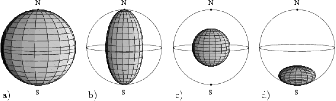
Figure 2: One qubit operations acting on the Bloch ball (a), bit flip with $p=0.5$ (b), depolarizing channel with $p=0.5$ (c) and a non–unital operation of amplitude damping with $p=0.75$ (d).

An alternative approach to the problem is obtained using the Stokes parametrisation, which involves Pauli matrices $\sigma_{k}$. Any state $\rho=({\mathbbm{1}}+{\vec{\tau}}\cdot{\vec{\sigma}})/2$, is characterized by the Bloch vector $\vec{\tau}$. If $\rho^{\prime}=\Phi(\rho)$ is represented by $\vec{\tau}^{\prime}$, then any linear dynamics inside the Bloch ball may be described by an affine transformation of the Bloch vector

$${\vec{\tau}}^{\prime}=t{\vec{\tau}}+{\vec{\kappa}},$$ (51)

where $t$ denotes a real matrix of size $3$, while $\vec{\kappa}=(\kappa_{x},\kappa_{y},\kappa_{z})$ is the translation vector. It determines the image of the ball center, $\Phi(\rho_{*})=({\mathbbm{1}}+{\vec{\kappa}}\cdot{\vec{\sigma}})/2$. For unital maps $\Phi(\rho_{*})=\rho_{*}$ so ${\vec{\kappa}}=0$. Any positive map sends the Bloch ball into an ellipsoid which may degenerate to an ellipse, an interval or a point. Out of $12$ real parameters in (51) $3$ eigenvalues of $tt^{\dagger}$ determine the size of the ellipsoid, $6$ related to the eigenvectors specify the orientation of its axis and the $3$ parameters of the vector $\vec{\kappa}$ characterize the position of its center.

The real matrix $t$ may be brought to the form, $t=O_{1}\eta O_{2}$, where $O_{i}\in O(3)$ and the diagonal matrix $\eta$ contains non-negative singular values of $t$. However, it is convenient to impose an extra condition that both orthogonal matrices represent proper rotations ($O_{i}\in SO(3)$), at the expense of allowing some components of the diagonal vector $\vec{\eta}$ to be negative. This decomposition is not unique: the moduli $|\eta_{i}|$ are equal to singular values of $t$ and the sign of the product $\eta_{x}\eta_{y}\eta_{z}={\rm det}(t)$ is fixed. However, the signs of any two components of $\vec{\eta}$ may be changed by conjugating the map with a Pauli matrix.

In general, for any one–qubit CP map $\Phi$ one may find unitary matrices $U$ and $W$ of size $2$ such that the unitarily similar operation ${\Phi}_{UW}$ defined by (44) is represented by the diagonal matrix $\eta$. For simplicity we may thus restrict ourselves to the maps for which the matrix $t$ is diagonal and consists of the damping (distortion) vector, ${\vec{\eta}}=(\eta_{x},\eta_{y},\eta_{z})$. In this case the ellipsoid has the form

$$\Bigl{(}\frac{x-\kappa_{x}}{\eta_{x}}\Bigl{)}^{2}+\Bigl{(}\frac{y-\kappa_{y}}{\eta_{y}}\Bigl{)}^{2}+\Bigl{(}\frac{z-\kappa_{z}}{\eta_{z}}\Bigl{)}^{2}=1.$$ (52)

The affine transformation (51) determines the superoperator $L$ of the map. Reshuffling the superoperator matrix according to (26) we obtain the dynamical matrix $D=L^{R}$ which corresponds to the map $\Phi_{{\vec{\eta}},{\vec{\kappa}}}$,

$$D=\frac{1}{2}\left[\begin{array}[]{cccc}1+\eta_{z}+\kappa_{z}&0&\kappa_{x}+i\kappa_{y}&\eta_{x}+\eta_{y}\\ 0&1-\eta_{z}+\kappa_{z}&\eta_{x}-\eta_{y}&\kappa_{x}+i\kappa_{y}\\ \kappa_{x}-i\kappa_{y}&\eta_{x}-\eta_{y}&1-\eta_{z}-\kappa_{z}&0\\ \eta_{x}+\eta_{y}&\kappa_{x}-i\kappa_{y}&0&1+\eta_{z}-\kappa_{z}\end{array}\right],$$ (53)

clearly a special case of (50). For unital maps ${\vec{\kappa}}=0$ and the matrix $D$ splits into two blocks and its eigenvalues are

$$d_{0,3}=\frac{1}{2}[1+\eta_{z}\pm(\eta_{x}+\eta_{y})]{\quad\rm and\quad}d_{1,2}=\frac{1}{2}[1-\eta_{z}\pm(\eta_{x}-\eta_{y})].$$ (54)

Hence if the Fujiwara–Algoet conditions FA99

$$(1\pm\eta_{z})^{2}\geq(\eta_{x}\pm\eta_{y})^{2}$$ (55)

are fulfilled, the dynamical matrix $D$ is positive definite and the corresponding positive map $\Phi_{\vec{\eta}}$ is CP. This condition shows that not all ellipsoids located inside the Bloch ball may be obtained by acting on the ball with a CP map - see recent papers on one qubit maps FA99 ; TCDGS99 ; KR01 ; Oi01 ; Wo01 ; Uh01 ; RSW02 ; VV02 .

Note that dynamical matrices of unital maps do commute, $[D_{\Phi_{\vec{\eta}}},D_{\Phi_{\vec{\zeta}}}]=0$. Hence they share the same set of eigenvectors. When reshaped they form the orthogonal set of Kraus operators consisting of the identity $\sigma_{0}={\mathbbm{1}}_{2}$, and the three Pauli matrices $\vec{\sigma}$. Thus the canonical form of an arbitrary one–qubit bistochastic map reads

$$\rho^{\prime}=\Phi_{\vec{\eta}}(\rho)=\sum_{i=0}^{3}d_{i}\sigma_{i}\rho\sigma_{i},$$ (56)

which explains the name Pauli channels.

For concreteness let us distinguish some one-qubit channels. We are going to specify their translation and distortion vectors, $\vec{\kappa}$ and $\vec{\eta}$, since with use of the transformation (44) we may bring the matrix $t$ to its diagonal form. Alternatively, the channels may be defined using the canonical Kraus form (34) in which Kraus operators are given by the eigenvalues and eigenvectors of the dynamical matrix, $A_{i}=\sqrt{d_{i}}\chi_{i}$. From (56) it follows that for any $N=2$ bistochastic map the Kraus operators are $A_{i}=\sqrt{d_{i}}\sigma_{i}$. For the decaying channel, (also called amplitude–damping channel), which is not bistochastic, the eigenvectors of the dynamical matrix give

$$A_{1}=\left[\begin{array}[c]{cc}1&0\\ 0&\sqrt{1-p}\end{array}\right]{\rm\quad and\quad}A_{2}=\left[\begin{array}[c]{cc}0&\sqrt{p}\\ 0&0\end{array}\right]\ .$$ (57)

Basic properties of some selected maps are collected in Table 4 and illustrated in Fig. 2.

Table 4: Exemplary one–qubit channels: distortion vector $\vec{\eta}$, translation vector $\vec{\kappa}$ equal to zero for unital channels, rescaled Kraus spectrum ${\vec{d}}^{\prime}$, and the Kraus rank $k$.

Channels	$\vec{\eta}$	$\vec{\kappa}$	unital	${\vec{d}}^{\prime}$	$k$
rotation	$(1,1,1)$	$(0,0,0)$	yes	$(1,0,0,0)$	$1$
phase flip	$(1-p,1-p,1)$	$(0,0,0)$	yes	$(1-p/2,p/2,0,0)$	$2$
decaying	$(\sqrt{1-p},\sqrt{1-p},1-p)$	$(0,0,p)$	no	$(1-p/2,p/2,0,0)$	$2$
depolarizing	$[1-x](1,1,1)$	$(0,0,0)$	yes	$\frac{1}{4}(4-3x,x,x,x)$	$4$
linear	$(0,0,q)$	$(0,0,0)$	yes	$\frac{1}{4}(1+q,1-q,$ $1-q,1+q)$	$4$
planar	$(0,r,q)$	$(0,0,0)$	yes	$\frac{1}{4}(1+q+r,1-q-r,$ $1-q+r,1+q-r)$	$4$

The geometry of the set of bistochastic maps is simplest to understand for $N=2$. As discussed in section V this set coincides LS93 with the set of $N=2$ random external fields (47), which may be defined as the convex hull of four unitary operations, $\sigma_{0}={\mathbbm{1}},\sigma_{x},\sigma_{y}$ and $\sigma_{z}$. Thus, in agreement with (56), any one-qubit bistochastic map $\Phi\in{\cal B}_{2}$ may be written as a convex combination of four matrices $\sigma_{j}$, $j=0,...,3$. Since $\sigma_{j}=-i\exp(i\pi\sigma_{j}/2)$, and the overall phase $-\pi$ is not relevant, each Pauli matrix represents the rotation of the Bloch ball around the corresponding axis by angle $\pi$. The distortion vectors ${\vec{\eta}}$ of four extremal maps $\sigma_{j}$ read $(1,1,1)$, $(1,-1,-1)$, $(-1,1,-1)$, and $(-1,-1,1)$, respectively. Hence, in accordance with the constraints (55), the set of bistochastic maps ${\cal B}_{2}$ written in the canonical form (with diagonal matrix $t$), forms a tetrahedron, see Fig. 3a. Its center is occupied by the completely depolarizing channel with ${\vec{\eta}}={\vec{0}}$, which may be expressed as a uniform mixture of four extremal unitarities; $\Psi_{*}=({\mathbbm{1}}+\sigma_{x}+\sigma_{y}+\sigma_{z})/4$. Interestingly, the set of non unital channels with a fixed translation vector ${\vec{\kappa}}\neq 0$ forms a convex set which resembles a tetrahedron with its corners rounded RSW02 .

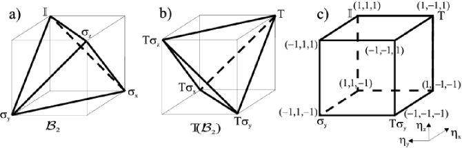
Figure 3: Subsets of one–qubit maps: a) set ${\cal B}_{2}$ of bistochastic maps (unital & CP), b) set $T({\cal B}_{2})$ of unital & CcP maps, c) set of positive (decomposable) unital maps.

Observe that in the generic case $|\eta_{i}|<1$, which suggests that a typical one-qubit CP map is a contraction. This is true also for higher dimensions, $N>2$. The monotone distances (e.g. the trace distance and the Bures distance NC00 ) do not increase under the action of CP maps. Apart from unitary (antiunitary) operations, for which these distances are preserved, the transformation inverse to a quantum operation is not an operation any more: some mixed states are sent outside the set of positive operators.

VII Positive & decomposable maps

Quantum transformations which describe physical processes are represented by completely positive maps. Why should we care about maps which are not completely positive? On one hand it is instructive to realize that seemingly innocent transformations are not CP, and thus do not correspond to any physical process. On the other hand maps which are positive, not completely positive provide a crucial tool in the investigation of entangled mixed states Per96 ; HHH96a ; HHH01 .

Consider the transposition of a density matrix in a certain basis $T:\rho\to\rho^{T}$. The corresponding superoperator $L_{T}$ entering (22) has the form $(L_{T})_{\stackrel{{\scriptstyle\scriptstyle m\mu}}{{n\nu}}}=\delta_{m\nu}\delta_{n\mu}$, and equals the dynamical matrix, $L_{T}=L_{T}^{R}=D_{T}$. This is a permutation matrix which contains $N$ diagonal entries equal to unity and $N(N-1)/2$ blocks of size two, Thus its spectrum, spec$(D_{T})$, consists of $N(N+1)/2$ eigenvalues equal to unity and $N(N-1)/2$ eigenvalues equal to $-1$, which is consistent with the constraint tr$D=N$. The matrix $D_{T}$ is not positive, so the transposition $T$ is not completely positive. Another way to reach this conclusion is to act with the extended map of partial transposition on the maximally entangled state (72) and to check that $[T\otimes{\mathbbm{1}}](|\psi\rangle\langle\psi|)$ has negative eigenvalues.

The transposition of an $N$–dimensional Hermitian matrix $D$, which changes the signs of the imaginary part of the elements $D_{ij}$, may be viewed as a reflection with respect to the $N(N+1)/2-1$ dimensional hyperplane, so the remaining $N(N-1)/2$ components do change their signs. As shown in Fig. 4 this geometrical interpretation is simple to visualize for $N=2$: the transposition corresponds to a reflection of the Bloch ball with respect to the $(x,z)$ plane - the $y$ coordinate changes its sign. Note that rotation of the Bloch ball around the $z$-axis by the angle $\pi$, realized by a unitary operation, $\rho\to\sigma_{z}\rho\sigma_{z}$, also exchanges the ’western’ and the ’eastern’ hemispheres, but is completely positive.

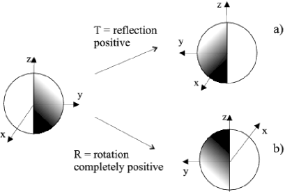
Figure 4: Non-contracting transformations of the Bloch ball: a) transposition (reflection with respect to the $x-z$ plane) - not completely positive; b) rotation by $\pi$ around $z$ axis - completely positive.

As discussed in section IV a given map $\Phi$ is not CP, if the corresponding dynamical matrix $D$ contains a negative eigenvalue. Let $m\geq 1$ denote the number of the negative eigenvalues (in short, the neg rank of $D$). Then the spectral decomposition of $D$ takes the form

$$D=\sum_{i=1}^{N^{2}-m}d_{i}|\chi_{i}\rangle\langle\chi_{i}|\ -\sum_{i=N^{2}-m+1}^{N^{2}}d_{i}|\chi_{i}\rangle\langle\chi_{i}|\ .$$ (58)

In analogy to the Kraus form (34) we may write the canonical form of a not completely positive map

$$\rho^{\prime}=\sum_{i=1}^{N^{2}-m}d_{i}\chi^{(i)}\rho(\chi^{(i)})^{\dagger}\ -\sum_{i=N^{2}-m+1}^{N^{2}}d_{i}\chi^{(i)}\rho(\chi^{(i)})^{\dagger},$$ (59)

where the Kraus operators $A_{i}=\sqrt{d_{i}}\chi^{(i)}$ form an orthonormal basis. The above form suggests that a positive map may be represented as a difference of two completely positive maps SS03 . Even though this statement is correct (for finite $N$), it does not solve the entire problem: taking any two CP maps and constructing a quasi-mixture (with negative weights allowed), $\Phi=(1+a)\Psi_{1}^{\rm CP}-a\Psi_{2}^{\rm CP}$, we do not know in advance how large the contribution $a$ of the negative part might be, to keep the map $\Phi$ positive… Although some criteria for positivity are known for several years St63 ; Ja74 ; Ma75 , they do not allow one to perform a practical test, whether a given map is positive. A recently proposed technique of extending the system (and the map) a certain number of times is shown to give a constructive test for positivity for a large class of maps DPS03 . In fact the characterization of the set ${\cal P}_{N}$ of positive maps: ${\cal M}^{(N)}\to{\cal M}^{(N)}$ is by far not simple and remains a subject of considerable mathematical interest St63 ; Cho72 ; Wo76b ; Cho80 ; TT83 ; Os92 ; Ky96 ; EK00 ; YH00 ; Ko00 ; MM01 ; LMM03 ; SS03 ; Ky03 . By definition, ${\cal P}_{N}$ contains the set ${\cal CP}_{N}$ of all CP maps as its proper subset.

To learn more about the set of positive maps we will need some other features of the operation of transposition $T$. For any operation $\Phi$ the modifications of the dynamical matrix induced by a composition with $T$ may be described by the partial transpose transformation

$$L_{T{\Phi}}=L_{\Phi}^{F_{1}},\quad D_{T{\Phi}}=D_{\Phi}^{T_{A}},\quad{\rm and}\quad L_{{\Phi}T}=L_{\Phi}^{F_{2}},\quad D_{{\Phi}T}=D_{\Phi}^{T_{B}}.$$ (60)

To demonstrate this it is enough to use the explicit form of $L_{T}$ and the following law of composition of dynamical matrices. Since the composition of two maps $\Psi\Phi$ results in the product of linear matrices,

$$L_{\Psi\Phi}=L_{\Psi}L_{\Phi},{\quad\rm hence\quad}D_{\Psi\Phi}=[D_{\Psi}^{R}D_{\Phi}^{R}]^{R}.$$ (61)

Even though the composition of two maps is usually written as $\Psi\cdot\Phi$, to simplify the notation the symbol $\cdot$ will often be dropped. Note that both operations commute, $\Psi\Phi=\Psi\Phi$, if $[D_{\Phi}^{R},D_{\Psi}^{R}]=0$.

Positivity of $D_{\Psi\Phi}$ follows also from the fact that the composition of two CP maps is completely positive. Alternatively one may prove the following reshuffling lemma

Consider two Hermitian matrices $A$ and $B$ of the same size $KN$.

$${\it If\quad}A\geq 0{\it\quad and\quad}B\geq 0{\it\quad then\quad}(A^{R}B^{R})^{R}\geq 0.$$ (62)

It was formulated in a different set up and proved in Ha03 .

The sandwiching of $\Phi$ between two actions of transpositions does not influence the spectrum of the dynamical matrix, $L_{T{\Phi}T}=L_{\Phi}^{F}=L_{\Phi}^{*}$ and $D_{T{\Phi}T}=D_{\Phi}^{T}=D_{\Phi}^{*}$. Thus if $\Phi$ is a CP map, so is $T\Phi T$, (if $D_{\Phi}$ is positive so is $D_{\Phi}^{T}$) – see Fig. 5.

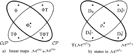
Figure 5: a) Sketch of the set of CP maps and of its image with respect to transposition: the set of CcP maps, b) the isomorphic sets of quantum states (dynamical matrices) and its image under the action of partial transposition.

The non completely positive map $T$ of transposition allows one to introduce the following definition St63 ; Cho75a ; Cho80 :

A map $\Phi$ is called completely co-positive (CcP), if the map $T\Phi$ is CP.

Properties (60) of the dynamical matrix imply that the map $\Phi T$ could be used instead to define the same set of CcP maps. Thus any CcP map may be written in a Kraus–like form

$$\rho^{\prime}=\sum_{i=1}^{k}A_{i}\rho^{T}A_{i}^{\dagger}.$$ (63)

Moreover, as shown in Fig. 5, the set ${\cal C}{\rm c}{\cal P}$ may be understood as the image of $\cal CP$ with respect to the transposition. Since we have already identified the transposition with a kind of reflection, it is rather intuitive to observe that the set ${\cal C}{\rm c}{\cal P}$ is a twin copy of ${\cal CP}$ with the same shape and volume. This property is easiest to analyze for the set ${\cal B}_{2}$ of one qubit bistochastic maps Oi01 . The dual set of CcP unital one qubit maps, $T({\cal B}_{2})$, forms a tetrahedron spanned by four maps $T\sigma_{i}$ for $i=0,1,2,3$, which is the reflection of the set of the bistochastic maps with respect to the center of the tetrahedron - the completely depolarizing channel $\Phi_{*}$ -see Fig. 3b. Observe that the corners of ${\cal B}_{2}$ are formed by proper rotations, for which det$(t)=\eta_{1}\eta_{2}\eta_{3}$ is equal to $+1$, while the extremal points of the set of CcP maps represent reflections for which det$(t)=-1$.

A positive map $\Phi$ is called decomposable, if it may be expressed as a convex combination of a CP map and a CcP map, $\Phi=a\Phi_{\rm CP}+(1-a)\Phi_{\rm CcP}$ with $a\in[0,1]$. A relation between CP maps acting on quaternion matrices and the decomposable maps defined on complex matrices was shown by Kossakowski Ko00 . An important characterization of the set ${\cal P}_{2}$ of positive maps acting on (complex) states of one qubit follows from the Størmer–Woronowicz theorem St63 ; Wo76b

Every one-qubit positive map $\Psi\in{\cal P}_{2}$ is decomposable.

In other words, the entire set of one qubit positive maps can be represented by the convex hull of the set of CP and CcP maps, ${\cal P}_{2}={\rm conv~{}~{}hull~{}}\Bigl{(}{\cal CP}_{2}\cup{\cal C}c{\cal P}_{2}\Bigr{)}$. This property, illustrated in Fig. 6, holds also for the maps ${\cal M}^{(2)}\to{\cal M}^{(3)}$ and ${\cal M}^{(3)}\to{\cal M}^{(2)}$ Wo76a , but is not true in higher dimensions, in particular in the sets ${\cal P}_{N}$ with $N\geq 3$. Consider a map defined on ${\cal M}^{(3)}$, depending on three non-negative parameters,

$$\Psi_{a,b,c}(\rho)\!=\!\left[\begin{array}[c]{ccc}a\rho_{11}+b\rho_{22}+c\rho_{33}&0&0\\ 0&c\rho_{11}+a\rho_{22}+b\rho_{33}&0\\ 0&0&b\rho_{11}+c\rho_{22}+a\rho_{33}\end{array}\right]-\rho.$$ (64)

The map $\Psi_{2,0,2}\in{\cal P}_{3}$ was a first example of a indecomposable map found by Choi in 1975 Cho75 in connection with positive biquadratic forms. As denoted schematically in Fig. 6b this map is extremal and belongs to the boundary of the convex set ${\cal P}_{3}$. The Choi map was generalized later in CL77 and in CKL92 , where it was shown that the map (64) is positive if and only if

$$a\geq 1,\quad a+b+c\geq 3,\quad 1\leq a\leq 2\Longrightarrow bc\geq(2-a)^{2},$$ (65)

while it is decomposable if and only if

$$a\geq 1,\quad 1\leq a\leq 3\Longrightarrow bc\geq(3-a)^{2}/4.$$ (66)

In particular, $\Psi_{2,0,c}$ is positive but not decomposable for $c\geq 1$. All generalized indecomposable Choi maps are known to be atomic HaKC98 , it is they cannot be written as a convex sum of $2$–positive and $2$–co–positive maps TT88 . An example of an indecomposable map belonging to ${\cal P}_{4}$ was given by Robertson Ro83 . A family of indecomposable maps for an arbitrary finite dimension $N\geq 3$ was recently found by Kossakowski Ko03 . They consist of an affine contraction of the set ${\cal M}^{(N)}$ of density matrices into the ball inscribed in it followed by a generic rotation from $O(N^{2}-1)$. Although several other methods of construction of indecomposable maps were proposed Tan86 ; TT88 ; Os91 ; KK94 , some of them in the context of quantum entanglement Te00 ; Yu00 ; HKP03 , the general problem of describing all positive maps remains open. In particular, it is not known, if one could find a finite set of $K$ positive maps $\{\Psi_{j}\}$, such that ${\cal P}_{N}={\rm conv~{}~{}hull~{}}\Bigl{(}\cup_{j=1}^{K}\Psi_{j}({\cal CP}_{N})\Bigr{)}$.

Due to the theorem of Størmer and Woronowicz the answer is known only for $N=2$, for which $K=2$, $\Psi_{1}={\mathbbm{1}}$ and $\Psi_{2}=T$. As emphasized by Horodeccy in an important work HHH96a these properties of the set ${\cal P}_{N}$ become decisive for the separability problem: the separability criterion based on the positivity of $({\mathbbm{1}}\otimes T)\rho$ works for the system of two qubits, but does not solve the problem in the general case of the $N\times N$ composite system.

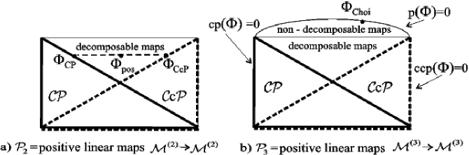
Figure 6: Sketch of the set positive maps: a) for $N=2$ all maps are decomposable, b) for $N>2$ there exist non-decomposable maps.

The indecomposable maps are worth investigating, since each such map provides a criterion for separability. Conditions for a positive map $\Phi$ to be decomposable were found some time ago by Størmer St82 . Since this criterion is not a constructive one, we describe here a simple test which may confirm the decomposability. Assume first that the map is not symmetric with respect to the transposition $\Phi\neq T\Phi$. These two different points determine a line in the space of maps, parametrized by $\beta$, along which we analyze the dynamical matrix

$$D_{\beta\Phi+(1-\beta)T\Phi}=\beta D_{\Phi}+(1-\beta)D_{\Phi}^{T_{A}}$$ (67)

and check its positivity by diagonalization. Assume that this matrix is found to be positive for some $\beta_{*}<0$ (or $\beta_{*}>1$), then the line (67) crosses the set of completely positive maps (see Fig. 7a). Since $D(\beta_{*})$ represents a CP map $\Psi_{\rm CP}$, hence $D(1-\beta_{*})$ defines a completely co–positive map $\Psi_{\rm CcP}$, and we find an explicit decomposition, $\Phi=[-\beta_{*}\Psi_{\rm CP}+(1-\beta_{*})\Psi_{\rm CcP}]/(1-2\beta_{*})$. In this way the decomposability of $\Phi$ may be established, but with this criterion one cannot confirm that a given map is indecomposable.

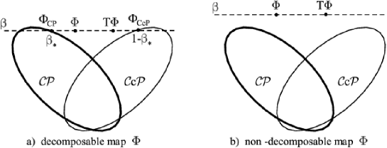
Figure 7: Geometric criterion to verify decomposability of a map $\Phi$: (a) if the line passing through $\Phi$ and $\Phi T$ crosses the set of completely positive maps, a decomposition of $\Phi$ is explicitly constructed.

To study the geometry of the set of positive maps it is convenient to work with the Hilbert–Schmidt distance, defined by the $HS$ norm of the difference between the superoperators, $d(\Psi,\Phi)=d_{HS}(L_{\Psi},L_{\Phi})=||L_{\Psi}-L_{\Phi}||_{HS}$. Since the reshuffling of a matrix does not influence its $HS$ norm, the distance can be measured directly in the space of dynamical matrices, $d(\Psi,\Phi)=d_{HS}(D_{\Psi},D_{\Phi})$. Note that for unital one qubit maps, (53) with ${\vec{\kappa}}=0$, one has $d(\Phi_{1},\Phi_{2})=|{\vec{\eta}}_{1}-{\vec{\eta}}_{2}|$, so Fig. 3 represents correctly the HS geometry of the space of $N=2$ unital maps.

In order to characterize, to what extent a given map $\Psi$ acting on ${\cal M}^{(N)}$ is close to the boundary of the set of positive (CP or CcP) maps, let us introduce the following quantities

$$\!\!{\bf a)} {\it\quad complete\quad positivity,\quad} cp(\Phi)\equiv\min_{{\cal M}^{(N)}}\langle\rho|D_{\Phi}|\rho\rangle,$$ (68)

$${\bf b)} {\it\ complete\ co\!-\!positivity,\ } ccp(\Phi)\equiv\min_{{\cal M}^{(N)}}\langle\rho|D^{T_{A}}_{\Phi}|\rho\rangle\ ,$$ (69)

$$\!\!{\bf c)} {\it\quad positivity,\quad} p(\Phi)\equiv\!\!\!\!\min_{x,y\in{\mathbb{C}}P^{N-1}}\!\!\![\langle x\otimes y|D_{\Phi}|x\otimes y\rangle].$$ (70)

The two first quantities may be easily found by diagonalization, $cp(\Phi)=\min\{{\rm eig}(D_{\Phi})\}$ and $ccp(\Phi)=\min\{{\rm eig}(D^{T_{A}}_{\Phi})\}$. Although $p(\Phi)\geq cp(\Phi)$ by construction the evaluation of positivity is more involved, since one needs to perform the minimization over the space of all product states, i.e. the Cartesian product ${\mathbb{C}}P^{N-1}\times{\mathbb{C}}P^{N-1}$. No straightforward method of computing this minimum is known, so one has to rely on numerical minimization. In certain cases this quantity was estimated analytically by Terhal Te00 and numerically by Gühne et al. GHDELMS02 ; GHDELMS03 in the context of characterizing the entanglement witnesses. In fact a non-positive dynamical matrix $D$, which describes a non completely positive map, may be just considered as an entanglement witnesses – an operator $D$ such Tr$D\rho$ is not negative for all separable states and negative for a given entangled state LKCHC00 ; LKHC01 ; Te02 ; Br02 ; PR03 .

As follows from the positivity of $D$ and $D^{T_{A}}$ and the property of block positivity (28), a given map $\Phi$ is completely positive (CcP, positive) if and only if the complete positivity (ccp, positivity) is non–negative. As marked in Fig. 6b, the relation $cp(\Phi)=0$ defines the boundary of the set ${\cal CP}_{N}$, while $ccp(\Phi)=0$ and $p(\Phi)=0$ define the boundaries of ${\cal C}c{\cal P}_{N}$ and ${\cal P}_{N}$. By direct diagonalization of the dynamical matrix we find that $cp({\mathbbm{1}})=ccp(T)=0$ and $ccp({\mathbbm{1}})=cp(T)=-1$.

For any not completely positive map $\Phi_{\rm nCP}$ one may look for its best approximation with a physically realizable $CP$ map $\Phi_{\rm CP}$, e.g. by minimizing their HS distance $d(\Phi_{\rm nCP},\Phi_{\rm CP})$ – see Fig. 9a. Such maps, called structural physical approximation were introduced in HE02 to propose an experimentally feasible scheme of entanglement detection and later studied in Fi02 .

To see a simple application of complete positivity, consider a non physical positive map with $cp(\Phi_{\rm nCP})=-x<0$. Its possible CP approximation, but generally not the optimal one, may be constructed out of its convex combination with the completely depolarizing channel $\Psi_{*}$. Diagonalizing the dynamical matrix representing the map $\Psi_{x}=a\Phi_{\rm nCP}+(1-a)\Psi_{*}$ with $a=1/(Nx+1)$ we see that its smallest eigenvalue is equal to zero, so $\Psi_{x}$ belongs to the boundary of ${\cal CP}_{N}$. Hence the distance $d(\Phi_{\rm nCP},\Phi_{x})$, which is a function of the complete positivity $cp(\Phi_{\rm nCP})$, gives an upper bound for the distance of $\Phi_{\rm nCP}$ from the set ${\cal CP}$. In a similar way one may use $ccP(\Phi)$ to obtain an upper bound for the distance of an analyzed non CcP map $\Phi_{\rm nCcP}$ from the set ${\cal C}c{\cal P}$. Interestingly, the solution of the analogous problem in the space of density matrices allows one to characterize the entanglement of a two-qubit mixed state $\rho_{1}$ by its minimal distance to the set of separable states. In the two–qubit system the entangled states do not have positive partial transpose, so $T_{A}(\rho_{1})$ is not a state. As shown in Fig. 9b one may also study a related problem of finding the state $\rho_{2}$ which is closest to $T_{A}(\rho_{1})$.

VIII Jamiołkowski isomorphism

Let ${\cal CP}_{N}$ denote the space of all trace preserving, completely positive maps $\Phi:{\cal M}^{(N)}\to{\cal M}^{(N)}$. Note that this is a convex set. Any such a map $\Phi$ may be uniquely represented by its dynamical matrix $D_{\Phi}$ of size $N^{2}$. It is a positive, Hermitian matrix and its trace is equal to $N$. Hence the rescaled matrix $\rho_{\Phi}\equiv D_{\Phi}/N$ represents a mixed state in ${\cal M}^{(N^{2})}$, and the entropy of the operation $S(\Phi)$ equals to the von Neumann entropy of $\rho_{\Phi}$. In fact rescaled dynamical matrices explore only a subspace of this set determined by the trace preserving conditions (27), which impose $N^{2}$ constraints. Let us denote this $N^{4}-N^{2}$ dimensional set by ${\cal M}_{I}^{(N^{2})}$. Since for any trace preserving CP map we may find a dynamical matrix, and vice versa, the correspondence between the maps from ${\cal CP}_{N}$ and the states of ${\cal M}_{I}^{(N^{2})}$ is one–to–one. In Table 5 this isomorphism is labeled by $J_{III}$.

Table 5: Jamiołkowski Isomorphism (73) between Hermicity reserving linear maps $\Phi$ definded on the space of mixed states ${\cal M}^{(N)}$ which act on ${\cal H}_{N}$ and the operators $D_{\Phi}$ on the composed space ${\cal H}_{N}\otimes{\cal H}_{N}$.

Isomorphism	Linear maps $\Phi:{\cal M}^{(N)}\to{\cal M}^{(N)}$	Hermitian operators $D_{\Phi}:{\cal H}_{N^{2}}\to{\cal H}_{N^{2}}$
$J_{I}$	positive maps $\Phi$	operators $D$ positive on product states
$J_{II}$	completely positive maps $\Phi$	positive operators $D$
$J_{III}$	quantum operations: CP, trace preserving maps	states $\rho=D/N$   such that Tr${}_{A}D={\mathbbm{1}}$
$J_{IIIa}$	completely positive,  unital maps	states $\rho=D/N$   such that Tr${}_{B}D={\mathbbm{1}}$
$J_{IV}$	CP and CcP trace preserving maps	mixed states $\rho=D/N$ such that Tr${}_{A}D={\mathbbm{1}}$ with positive partial transpose
example of $J_{IV}$ for $N=2$	CP and CcP trace preserving maps $\Phi:{\cal M}^{(2)}\to{\cal M}^{(2)}$	separable states $\rho=D/N$ of a $2\times 2$ composite system such that Tr${}_{A}D={\mathbbm{1}}$
$J_{IVa}$	unitary rotations $\rho^{\prime}=U\rho U^{\dagger}$, $D_{\Phi}=(U\otimes U^{*})^{R}$	maximally entangled pure states $(U\otimes{\mathbbm{1}})|\psi\rangle\langle\psi|$
$N=2$ example of $J_{IVa}$	${\mathbbm{1}}\leftrightarrow(1,0,0,1)$	$|\psi_{+}\rangle\equiv\frac{1}{\sqrt{2}}|00\rangle+|11\rangle$
Pauli matrices	${\sigma_{x}}\leftrightarrow(0,1,1,0)$	$|\phi_{+}\rangle\equiv\frac{1}{\sqrt{2}}|01\rangle+|10\rangle$
versus	${\sigma_{y}}\leftrightarrow(0,-i,i,0)$	$|\phi_{-}\rangle\equiv\frac{1}{\sqrt{2}}|01\rangle-|10\rangle$
Bell states $\rho_{\phi}=|\phi\rangle\langle\phi|$	${\sigma_{z}}\leftrightarrow(1,0,0,-1)$	$|\psi_{-}\rangle\equiv\frac{1}{\sqrt{2}}|00\rangle-|11\rangle$
$J_{V}$	completely depolarizing channel $\Phi_{*}$	maximally mixed state $\rho_{*}={\mathbbm{1}}/N$

Let us find the dynamical matrix for the identity operator, $L={\mathbbm{1}}_{N^{2}}$,

$$L^{\mathbbm{1}}_{\stackrel{{\scriptstyle\scriptstyle m\mu}}{{n\nu}}}=\delta_{mn}\delta_{\mu\nu}{\quad\rm so\quad that\quad}D^{\mathbbm{1}}_{\stackrel{{\scriptstyle\scriptstyle m\mu}}{{n\nu}}}=(L^{\mathbbm{1}}_{\stackrel{{\scriptstyle\scriptstyle m\mu}}{{n\nu}}})^{R}=\delta_{m\mu}\delta_{n\nu}=N\rho^{\psi}_{\stackrel{{\scriptstyle\scriptstyle m\mu}}{{n\nu}}},$$ (71)

where $\rho^{\psi}=|\psi\rangle\langle\psi|$ represents the operator of projection on the maximally entangled state of the composite system

$$|\psi\rangle=\sum_{i=1}^{N}\frac{1}{\sqrt{N}}|i\rangle\otimes|i\rangle.$$ (72)

This state is written in its Schmidt form Pe95b (for $N=2$ it is the famous Bell state), and we see that all its Schmidt coefficients are equal, $\lambda_{1}=\lambda_{i}=\lambda_{N}=1/N$. Thus we have found that the identity operator corresponds to the maximally entangled pure state $|\psi\rangle\langle\psi|$ of the composite system. Interestingly, this correspondence may be extended for other operations, or in general, for arbitrary linear maps. Any linear map $\Phi$ acting on the space of mixed states ${\cal M}^{(N)}$ can be associated, via its dynamical matrix $D_{\Phi}$, with an operator acting in the enlarged Hilbert state ${\cal H}_{N}\otimes{\cal H}_{N}$

$$\Phi:{\cal M}^{(N)}\to{\cal M}^{(N)}\quad\longleftrightarrow\quad D_{\Phi}=N\bigl{[}\Phi\otimes{\mathbbm{1}}\bigr{]}(|\psi\rangle\langle\psi|)$$ (73)

To show this we represent the linear map $\Phi$ by its matrix $L$ introduced in (22), write the operator $\Phi\otimes{\mathbbm{1}}$ as an eight–indices matrix and study its action on the state $\rho^{\psi}$ expressed by (71),

$$L_{\stackrel{{\scriptstyle\scriptstyle mn}}{{m^{\prime}n^{\prime}}}}{\mathbbm{1}}_{\stackrel{{\scriptstyle\scriptstyle\mu\nu}}{{\mu^{\prime}\nu^{\prime}}}}N\rho^{\psi}_{\stackrel{{\scriptstyle\scriptstyle m^{\prime}\mu^{\prime}}}{{n^{\prime}\nu^{\prime}}}}=L_{\stackrel{{\scriptstyle\scriptstyle mn}}{{\mu\nu}}}=D_{\stackrel{{\scriptstyle\scriptstyle m\mu}}{{n\nu}}}.$$ (74)

An analogous operation ${\mathbbm{1}}\otimes\Phi$ acting on $\rho^{\psi}$ leads to the matrix $D^{F}$ with the same spectrum. Conversely, for any positive matrix $D$ we find the corresponding map $\Phi$ by diagonalization. The reshaped eigenvectors $|\chi_{i}\rangle$ of $D$, rescaled by the roots of its eigenvalues give the canonical Kraus form (30,34) of the corresponding operation $\Phi$. Furthermore, the entropy of the quantum operation $S(\Phi)$ equals the von Neumann entropy $S(\rho_{\Phi})$ of the corresponding state $\rho_{\Phi}=D_{\Phi}/N$.

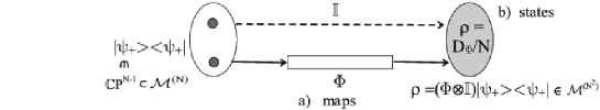
Figure 8: Duality between quantum map $\Phi$ acting on a part of the maximally entangled state $|\psi_{+}\rangle$ and the resulting density matrix $\rho=\frac{1}{N}D_{\Phi}$

Consider now a more general case in which $\rho$ denotes a state acting on a composite Hilbert space ${\cal H}_{N}\otimes{\cal H}_{N}$. Let $\Phi$ be an arbitrary map which sends ${\cal M}^{(N)}$ into itself and let $D_{\Phi}=L^{R}_{\Phi}$ denote its dynamical matrix (of size $N^{2}$). Acting with the extended map on $\rho$ we find its image $\rho^{\prime}=[\Phi\otimes{\mathbbm{1}}](\rho)$. Writing down the explicit form of the corresponding linear map in analogy to (74), and contracting over the four indices representing $\mathbbm{1}$, we obtain

$$(\rho^{\prime})^{R}=L_{\Phi}\rho^{R}{\quad\rm so\quad that\quad}\rho^{\prime}=(D_{\Phi}^{R}\rho^{R})^{R}.$$ (75)

In the above formula the standard multiplication of square matrices takes place, in contrast to Eq. (22) in which the state $\rho$ acts on a simple Hilbert space and is treated as a vector.

Note that Eq. (73) may be obtained as a special case of (75) if one takes for $\rho$ the maximally entangled state (72), for which $(\rho^{\psi})^{R}={\mathbbm{1}}$. Formula (75) provides a useful application of the dynamical matrix corresponding to a map $\Phi$ acting on a subsystem. Since the normalization of matrices does not influence positivity, this result implies the reshuffling lemma (62).

Formula (73) may also be used to find operators $D$ associated with positive maps $\Phi$ which are neither trace preserving nor complete positive. The correspondence between the set of positive linear maps and dynamical matrices acting in the composite space and positive on product states is called Jamiołkowski isomorphism since it follows from his results obtained in Ja72 . Some aspects of the duality between maps and states were recently investigated in Ha03 ; AP03b . Let us mention here explicitly certain special cases of this isomorphism labeled by $J_{I}$ in Table 5. The set of all completely positive maps $\Phi$ is isomorphic to the set of all positive matrices $D$, (case $J_{II}$). Unital CP maps are related to dynamical matrices which satisfy ${\rm tr}_{B}D={\mathbbm{1}}$ (case $J_{IIIa}$). The set of all quantum operation, (i.e. the trace preserving, CP maps) corresponds to the set of positive matrices $D$ fulfilling another constraint, ${\rm tr}_{A}D={\mathbbm{1}}$ – see Table 5, item $J_{III}$. An apparent asymmetry between the role of both subsystems is due to the particular choice of the relation (73); if the operator ${\mathbbm{1}}\otimes\Phi$ is used instead, the subsystems $A$ and $B$ in the partial trace constraints need to be interchanged.

An important case $J_{IV}$ of the isomorphism concerns the states with positive partial transpose, $\rho^{T_{A}}\geq 0$. called briefly PPT states. Another case, $J_{IVa}$, relates the set of unitary rotations, $\rho^{\prime}=\Phi(\rho)=U\rho U^{\dagger}$ with the maximally entangled states, $(U\otimes{\mathbbm{1}})\bigr{|}\psi\rangle\langle\psi|$. The local unitary operation $(U\otimes{\mathbbm{1}})$ preserves the purity of a state and its Schmidt coefficients. Thus the set of unitary matrices $U$ of size $N$ is isomorphic to the set of the maximally entangled pure states of the composite $N\times N$ system. In particular, vectors obtained by reshaping the Pauli matrices $\sigma_{i}$ represent the Bell states in the computational basis, as listed in Table 5. Eventually, case $J_{V}$ consists of a single, distinguished point in both spaces: the completely depolarizing channel $\Phi_{*}$ and the corresponding maximally mixed state $\rho_{*}$. Note the following inclusion relations of the sets mentioned in Table 5, $J_{I}\supset J_{II}\supset J_{III}\supset J_{IV}\supset J_{V}\subset J_{IIIa}$ and $J_{II}\supset J_{IIIa}\supset J_{IVa}\subset J_{III}$, as sketched in Fig. 9.

IX Quantum maps and quantum states

Relation (73) allows one to link an arbitrary linear map $\Phi$ with the corresponding linear operators given by the dynamical matrix $D_{\Phi}$. Expressing the maximally entangled state $|\psi\rangle$ in (73) by its Schmidt form (72) we may compute the matrix elements of $D_{\Phi}$ in the product basis consisting of the states $|i\otimes j\rangle$. Due to the factorization of the right hand side we see that the double sum describing $\rho_{\Phi}=D_{\Phi}/N$ drops out and the result reads

$$\langle k\otimes i|D_{\Phi}|l\otimes j\rangle=\langle k\bigl{|}\Phi(|i\rangle\langle j|)\bigr{|}l\rangle.$$ (76)

This equation may also be understood as a definition of a map $\Phi$ related to the linear operator $D_{\Phi}$. It proves the isomorphism $J_{I}$ from Table 5: if $D_{\Phi}$ is block positive, then the corresponding map $\Phi$ sends positive operators into positive operators Ja72 .

As listed in Table 5 and shown in Fig. 9 the Jamiołkowski isomorphism (76) may be applied in various setups AP03b . Relating linear maps from ${\cal P}_{N}$ with the operators acting on an extended space ${\cal H}_{N}\otimes{\cal H}_{N}$ we may compare:

i) individual objects, e.g. completely depolarizing channel $\Phi_{*}$ and the maximally mixed state $\rho_{*}$,

ii) families of objects, e.g. the depolarizing channels and the Werner states We89 ,

iii) entire sets, e.g. the set of ${\cal CP}\cup{\cal C}c{\cal P}$ maps and the set of PPT states,

iv) certain problems, e.g. for an arbitrary CP map $\Phi$ find the closest CcP map, and the problem of finding the PPT state (separable state for $N=2$) closest to an arbitrary (entangled) state,  and

v) their solutions…

To get some more experience concerning the analyzed duality between quantum maps and quantum states compare both sides of Fig. 9. Note that this illustration may also be considered as a strict representation of a fragment of the space of one–qubit unital maps (a) or the space of two-qubits density matrices in the HS geometry (b). It is nothing else but the cross–section of the cube representing the positive maps in Fig. 3c along the plane determined by ${\mathbbm{1}},T$ and $\Phi_{*}$.

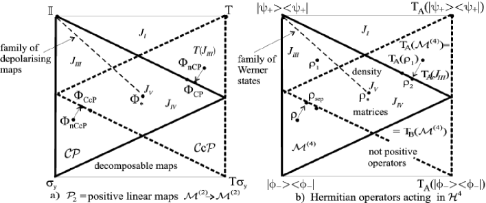
Figure 9: Isomorphism between objects, sets, and problems: a) linear one qubit maps, b) linear operators acting in two-qubit Hilbert space ${\cal H}_{4}$. Labels $J_{i}$ refer to the sets related by the isomorphisms defined in Table 5.

Let us finish this section by pointing out an analogue of the Jamiołkowski isomorphism in the classical case. The space of all classical states – probability vectors of size $N$ – forms the $N-1$ dimensional simplex $\Delta_{N-1}$. A discrete dynamics in this space is given by a stochastic transition matrix $T_{N}:\Delta_{N-1}\to\Delta_{N-1}$. It contains non–negative entries, and due to stochasticity the sum of all its elements is equal to $N$. Hence reshaping the transition matrix $T_{N}$ and rescaling it by $1/N$ we receive a probability vector ${\vec{t}}$ of length $N^{2}$. The classical states defined in this way form a measure zero, $N(N-1)$ dimensional, convex subset of $\Delta_{N^{2}-1}$. Consider, for instance, the set of $N=2$ stochastic matrices, which can be parametrized as $T_{2}=\left[\begin{array}[c]{cc}a&b\\ 1-a&1-b\end{array}\right]$ with $a,b\in[0,1]$. The set of the corresponding probability vectors ${\vec{t}}=(a,b,1-a,1-b)/2$ forms a square of size $1/2$ – the maximal square which may be inscribed into the unit tetrahedron $\Delta_{3}$ of all $N=4$ probability vectors.

The classical dynamics may be considered as a (very) special subclass of quantum dynamics, defined on the set of diagonal density matrices. Hence the classical and quantum duality between maps and states may be succinctly summarized in the following, commutative diagram

$$\begin{array}[]{llcl}{\rm quantum:}&\bigr{[}\Phi:{\cal M}^{(N)}\rightarrow{\cal M}^{(N)}\bigl{]}&\longrightarrow&D_{\Phi}\in{\cal M}^{(N^{2})}\\ &\quad\quad{\vphantom{\Bigg{|}}\downarrow}{\quad\rm maps}&&{\vphantom{\Bigg{|}}\downarrow}{\quad\rm states}\\ {\rm classical:}&\bigr{[}T:\Delta_{N-1}\rightarrow\Delta_{N-1}\bigl{]}&\longrightarrow&\ {\vec{t}}\ \in\Delta_{N^{2}-1}\ .\end{array}$$ (77)

Alternatively, vertical arrows may be interpreted as the action of the coarse graining operation $\Psi_{\rm CG}$ defined in section V. For instance, for the trivial (do nothing) one–qubit quantum map $\Phi_{\mathbbm{1}}$, the superoperator $L={\mathbbm{1}}_{4}$ restricted to diagonal matrices gives the identity matrix, $T={\mathbbm{1}}_{2}$, and the classical state ${\vec{t}}=(1,0,0,1)/2\in\Delta_{3}$. On the other hand, this very vector represents the diagonal of the maximally entangled state $\frac{1}{2}D_{\Phi}=|\psi\rangle\langle\psi|$. To prove the commutativity of the diagram (77) in the general case define the stochastic matrix $T$ as a submatrix of the superoperator (22), $T_{mn}=L_{\stackrel{{\scriptstyle\scriptstyle mm}}{{nn}}}$ (left vertical arrow). Note that the vector $\vec{t}$ obtained by its reshaping satisfies ${\vec{t}}={\rm diag}(L^{R})={\rm diag}(D_{\Phi})$, so it represents the diagonal of the dynamical matrix (right arrow).

X Envoi

In this work we analyzed the space ${\cal P}_{N}$ of positive maps, which send the set of mixed quantum states ${\cal M}^{(N)}$ into itself, and its various subsets: the set ${\cal CP}_{N}$ of completely positive maps, and the set ${\cal B}_{N}$ of bistochastic maps. For any quantum map $\Psi$ we have introduced three quantities, (68-70), to characterize the location of $\Psi$ with respect to the boundaries of the sets of positive (completely positive or completely co-positive) maps. We have defined and investigated the set of unistochastic maps, the elements of which are determined by a unitary matrix $U$ of size $N^{2}$ and correspond to the coupling with the $N$-dimensional environment, initially in the maximally mixed state.

The spaces of quantum maps (stochastic, bistochastic, unitary evolutions), which act on the set ${\cal M}^{(N)}$ of mixed quantum states, may be related with the corresponding classical maps (stochastic, bistochastic, permutations), which act on the simplex $\Delta_{N-1}$ of all $N$–point probability distributions. We have extended the Jamiołkowski isomorphism, linking the space of quantum maps with the space of bipartite quantum states, to the classical case (77).

In general the state–map duality, analyzed in this paper, may be formulated and applied in a variety of contexts and set ups. For instance, the set of $SU(4)$ matrices may be considered as:

a) the space of maximally entangled states of a composite, $4\times 4$ system, $|\psi\rangle\in{\mathbb{C}}P^{15}\subset{\cal M}^{(16)}$,

b) the set of two-qubit unitary gates acting on ${\cal M}^{(4)}$ - see e.g. KC01 ; HVC02 ; ZVWS03 ; NDDGMOBHH02 ,

c) the set ${\cal BU}_{2}$ of one qubit unistochastic operations (21), $\Psi_{U}\in{\cal BU}_{2}\subset{\cal B}_{2}\subset{\cal CP}_{2}$.

To conclude, we would like to convey two main points. On one hand, the set of positive maps has an interesting geometry, which is worthy of investigation in the general case $N\geq 3$. On the other hand, the marvelous duality between quantum maps and quantum states, based on the Jamiołkowski isomorphism, allows one to apply all the knowledge gained in studying the set of quantum maps to describe the set of quantum states (or conversely). For instance, the known structure of the set of completely positive maps relates to the structure of all quantum states, while the description of the (larger) set of all positive maps would allow us to describe the subset of all separable states.

It is a pleasure to thank R. Alicki, R. Dobrzański–Demkowicz, T. Havel, P. Horodecki, R. Horodecki, A. Kossakowski, M. Kuś, W. A. Majewski and F. Mintert for fruitful discussions and helpful comments. Financial support by Komitet Badań Naukowych under the grant PBZ-Min-008/P03/03 and Swedish grant from VR is gratefully acknowledged.

References

- [1] J. Åberg. Subspace preserving completely positive maps. preprint quant-ph, page 0302180, 2003.
- [2] L. Accardi. Nonrelativistic quantum mechanic as a noncommutative Markof process. Adv. Math., 20:329, 1976.
- [3] G. Alber, T. Beth, M. Horodecki, P. Horodecki, R. Horodecki, M. Rötteler, H. Weinfurter, R. Werner, and A. Zeilinger. Quantum Information: An Introduction to Basic Theoretical Concepts and Experiments. Springer, Berlin, 2001. Springer Tracts in Modern Physics.
- [4] S. Albeverio, K. Chen, and S.-M. Fei. Generalized reduction criterion for separability of quantum states. Phys. Rev., A 68:062313, 2003.
- [5] R. Alicki and M. Fannes. Quantum Dynamical Systems. Oxford University Press, Oxford, 2001.
- [6] R. Alicki and K. Lendi. Quantum Dynamical Semigroups and Applications. Springer–Verlag, Berlin, 1987.
- [7] G. G. Amosov, A. S. Holevo, and R. F. Werner. On some additivity problems in quantum information theory. preprint math-ph/0003002, 2000.
- [8] P. Arrighi and C. Patricot. On quantum operations as quantum states. preprint quant-ph, /:0307024, 2003.
- [9] W. B. Arveson. Subalgebras of –algebras. Acta Math., 123:141, 1969.
- [10] Arvind, K. S. Mallesh, and N. Mukunda. A generalized Pancharatnam geometric phase formula for three-level quantum systems. J. Phys., A 30:2417, 1997.
- [11] C. Beck and F. Schlögl. Thermodynamics of Chaotic Systems. Cambridge University Press, Cambridge, 1993.
- [12] D. Bouwmeester, A. K. Ekert, and A. Z. (eds.). The Physics of Quantum Information: Quantum cryptography, Quantum Teleportation, Quantum Computation. Springer, Berlin, 2000.
- [13] H.-P. Breuer and F. Petruccione. The Theory of Open Quantum Systems. Oxford University Press, Oxford, 2002.
- [14] D. Bruß. Characterizing entanglement. J. Math. Phys., 43:4237, 2002.
- [15] M. S. Byrd and N. Khaneja. Characterization of the positivity of the density matrix in terms of the coherence vector representation. quant-ph, page 03002024, 2003.
- [16] K. Chen and L.-A. Wu. A matrix realignment method for recognizing entanglement. Quant. Inf. Comp., 3:193, 2003.
- [17] S.-J. Cho, S.-H. Kye, and S. G. Lee. Generalized Choi map in -dimensional matrix algebra. Linear Alg. Appl., 171:213, 1992.
- [18] M.-D. Choi. Positive linear maps on –algebras. Can. J. Math., 3:520, 1972.
- [19] M.-D. Choi. Completely positive linear maps on complex matrices. Linear Alg. Appl., 10:285, 1975.
- [20] M.-D. Choi. Positive semidefinite biquadratic forms. Linear Alg. Appl., 12:95, 1975.
- [21] M.-D. Choi. Some assorted inequalities for positive maps on -algebras. J. Operator Theory, 4:271, 1980.
- [22] M.-D. Choi and T. Lam. Extremal positive semidefinite forms. Math. Ann., 231:1, 1977.
- [23] E. B. Davies. Quantum Theory of Open Systems. Academic Press, London, 1976.
- [24] A. C. Doherty, P. A. Parillo, and F. M. Spedalieri. A complete family of separability criteria. quant-ph, 1:0308032, 2003.
- [25] M.-H. Eom and S.-H. Kye. Duality for positive linear maps in matrix algebras. Math. Scand., 86:130, 2000.
- [26] D. E. Evans. Quantum dynamical semigroups. Acta Appl. Math., 2:333, 1984.
- [27] D. E. Evans and J. T. Levis. Dilatations of irreversible evolutions in algebraic quantum theories. Comm. Dublin. Inst. Adv. Studies, A 24:., 1977.
- [28] J. Fiurášek. Structural physical approximations of unphysical maps and generalized quantum measurements. Phys. Rev., A 66:052315, 2002.
- [29] A. Fujiwara and P. Algoet. One–to–one parametrization of quantum channels. Phys. Rev., A 59:3290, 1999.
- [30] J. Gruska. Quantum conputing. McGraw–Hill, New York, 1999.
- [31] O. Gühne, P. Hyllus, D. Bruß, A. Ekert, M. Lewenstein, C. Macchiavello, and A. Sanpera. Detection of entanglement with few local measurements. Phys. Rev., A 66:062305, 2002.
- [32] O. Gühne, P. Hyllus, D. Bruß, A. Ekert, M. Lewenstein, C. Macchiavello, and A. Sanpera. Experimental detection of entanglement via witness operators and local measurements. J. Mod. Opt., 50:1079, 2003.
- [33] K.-C. Ha. Atomic positive linear maps in matrix algebra. Publ. RIMS Kyoto Univ., 34:591, 1998.
- [34] K.-C. Ha, S.-H. Kye, and Y.-S. Park. Entangled states with positive partial transposes arising from indecomposable positive linear maps. preprint quant-ph, page 0305005, 2003.
- [35] K. Hammerer, G. Vidal, and J. I. Cirac. Characterization of non–local gates. Phys. Rev., A 66:062321, 2002.
- [36] T. F. Havel. Robust procedures for converting among Lindblad, Kraus and matrix representations of quantum dynamical semigroups. J. Math. Phys., 44:534, 2003.
- [37] M. Horodecki, P. Horodecki, and R. Horodecki. Separability of mixed states: necessary and sufficient conditions. Phys. Lett., A 223:1, 1996.
- [38] M. Horodecki, P. Horodecki, and R. Horodecki. Separability of n-particle mixed states: necessary and sufficient conditions in terms of linear maps. Phys. Lett., A 283:1, 2001.
- [39] M. Horodecki, P. Horodecki, and R. Horodecki. Separability of mixed quantum states: linear contractions approach. quant-ph, page 0206008, 2002.
- [40] M. Horodecki, P. Horodecki, and J. Oppenheim. Reversible transformations from pure to mixed states and the unique measure of information. Phys. Rev., A 67:062104, 2003.
- [41] P. Horodecki. From entanglement witnesses to positive maps: towards optimal characterisation of separability. In T. Gonis and P. E. A. Turchi, editors, Decoherence and its Implications in Quantum Computation and Quantrum Computing. IOS Press, 2001.
- [42] P. Horodecki and A. Ekert. Method for direct detection of quantum entanglement. Phys. Rev. Lett., 89:127902, 2002.
- [43] R. Ingarden. Quantum information theory. Rep. Math. Phys., 10:43, 1975.
- [44] R. Ingarden and A. Kossakowski. An axiomatic definition of information in quantum mechanics. Bull. Acad. Polon. Sci. Sér. math. astr. phys., 16:61, 1968.
- [45] R. Ingarden, A. Kossakowski, and M. Ohya. Information Dynamics and Open Systems. Kluver, Dordrecht, 1997.
- [46] R. Ingarden and K. Urbanik. Quantum informational thermodynamics. Acta Phys. Polon., 21:281, 1962.
- [47] L. Jakóbczyk and M. Siennicki. Geometry of Bloch vectors in two–qubit system. Phys. Lett., A 286:383, 2001.
- [48] A. Jamiołkowski. Linear transformations which preserve trace and positive semidefiniteness of operators. Rep. Math. Phys., 3:275, 1972.
- [49] A. Jamiołkowski. An effective method of investigation of positive maps on the set of positive definite operators. Rep. Math. Phys., 5:415, 1975.
- [50] M. Keyl. Fundamentals of quantum information theory. Phys. Rep., 369:431, 2002.
- [51] H.-J. Kim and S.-H. Kye. Indecomposable extreme positive linear maps in matrix algebras. Bull. London. Math. Soc., 26:575, 1994.
- [52] G. Kimura. The Bloch vector for –level systems. Phys. Lett., A 314:339, 2003.
- [53] C. King and M. B. Ruskai. Minimal entropy of states emerging from noisy channels. IEEE Trans. Inf. Th., 47:192, 2001.
- [54] E. Knill and R. Laflamme. Power of one bit of quantum information. Phys. Rev. Lett., 81:5672, 1998.
- [55] A. Kossakowski. On the quantum informational thermodynamics. Bull. Acad. Polon. Sci. Sér. math. astr. phys., 17:349, 1969.
- [56] A. Kossakowski. Remarks on positive maps of finite dimensional simple Jordan algebras. Rep. Math. Phys., 46:393, 2000.
- [57] A. Kossakowski. A class of linear positive maps in matrix algebras. Open Sys. & Information Dyn., 10:1, 2003.
- [58] B. Kraus and J. I. Cirac. Optimal creation of entanglement using a two-qubit gate. Phys. Rev., A 63:062309, 2001.
- [59] K. Kraus. General state changes in quantum theory. Ann. Phys., 64:311, 1971.
- [60] K. Kraus. States, Effects and Operations: Fundamental Notions of Quantum Theory. Springer-Verlag, Berlin, 1983.
- [61] S.-H. Kye. Facial structures for positive linear maps between matrix algebras. Canad. Math. Bull., 39:74, 1996.
- [62] S.-H. Kye. Facial structures for unital positive linear maps in the two dimensional matrix algebra. Linear Alg. Appl., 362:57, 2003.
- [63] L. E. Labuschagne, W. A. Majewski, and M. Marciniak. On k-decomposability of positive maps. math-ph, .:0306017, 2003.
- [64] L. J. Landau and R. F. Streater. On Birkhoff theorem for doubly stochastic completely positive maps of matrix algebras. Linear Algebra Appl., 193:107, 1993.
- [65] M. Lewenstein, B. Kraus, J. I. Cirac, and P. Horodecki. Optimization of entanglement witnesses. Phys. Rev., A 62:052310, 2000.
- [66] M. Lewenstein, B. Kraus, P. Horodecki, and J. I. Cirac. Characterization of separable states and entanglement witnesses. Phys. Rev., A 63:044304, 2001.
- [67] G. Lindblad. Completely positive maps and entropy inequalities. Commun. Math. Phys., 40:147, 1975.
- [68] G. Lindblad. On the generators of quantum dynamical semigroups. Commun. Math. Phys., 48:119, 1976.
- [69] G. Mahler and V. A. Weberrusß. Quantum Networks. Springer, Berlin, 1995, (II ed.) 1998.
- [70] W. A. Majewski. Transformations between quantum states. Rep. Math. Phys., 8:295, 1975.
- [71] W. A. Majewski and M. Marciniak. On characterization of positive maps. J. Phys., A 34:5863, 2001.
- [72] A. W. Marshall and I. Olkin. Inequalities: Theory of Majorization and its Applications. Academic Press, New York, 1979.
- [73] M. Musz, M. Kuś, and K. Życzkowski. Unitary quantum gates: a measure theoretic approach. to be published, 2004.
- [74] M. A. Nielsen and I. L. Chuang. Quantum Computation and Quantum Information. Cambridge University Press, Cambridge, 2000.
- [75] M. A. Nielsen, C. Dawson, J. Dodd, A. Gilchrist, D. Mortimer, T. Osborne, M. Bremner, A. Harrow, and A. Hines. Quantum dynamics as physical resource. Phys. Rev., A 67:052301, 2003.
- [76] M. Ohya and D. Petz. Quantum Entropy and Its Use. Springer, Berlin, 1993.
- [77] D. K. L. Oi. The geometry of single qubit maps. preprint quant-ph/0106035, 2001.
- [78] H. Osaka. Indecomposable positive maps in low dimensional matrix algebra. Linear Alg. Appl., 153:73, 1991.
- [79] H. Osaka. A class of extremal positive maps in matrix algebras. Publ. RIMS. Kyoto Univ., 28:747, 1992.
- [80] C. J. Oxenrider and R. D. Hill. On the matrix reordering and . Linear Alg. Appl., 69:205, 1985.
- [81] A. Peres. Quantum Theory: Concepts and Methods. Kluver, Dodrecht, 1995.
- [82] A. Peres. Separability criterion for density matrices. Phys. Rev. Lett., 77:1413, 1996.
- [83] A. O. Pittenger and M. H. Rubin. Geometry of entanglement witnesses and local detection of entanglement. Phys. Rev., A 67:012327, 2003.
- [84] J. A. Poluikis and R. D. Hill. Completely positive and hermitian–preserving transformations. Linear Algebra Appl., 35:1, 1981.
- [85] D. Poulin, R. Blume–Kohout, R. Laflamme, and H. Olivier. Exponential speed–up with a single bit of quantum information. quanty-ph, page 10038, 2003.
- [86] A. G. Robertson. Automorphisms of spin factors and the decomposition of positive maps. Quart. J. Math. Oxford, 34:87, 1983.
- [87] O. Rudolph. Further results on the cross norm criterion for separability. preprint quant-ph/0202121, 2002.
- [88] O. Rudolph. Some properties of the computable cross norm criterion for separability. Physical Review, A 67:032312, 2003.
- [89] M. B. Ruskai, S. Szarek, and E. Werner. An analysis of completely–positive trace–preserving maps on matrices. Linear Algebra Appl., 347:159, 2002.
- [90] W. F. Stinespring. Positive functions on algebras. Proc. Am. Math. Soc., 6:211, 1955.
- [91] E. Størmer. Positive linear maps of operator algebras. Acta Math., 110:233, 1963.
- [92] E. Størmer. Decomposable positive maps on -algebras. Proc. Amer. Math. Soc., 86:402, 1982.
- [93] J. Stryła. Stochastic quantum dynamics. arXive preprint quant-ph/0204161, 2002.
- [94] E. C. G. Sudarshan, P. M. Mathews, and J. Rau. Stochastic dynamics of quantum–mechanical systems. Phys. Rev., 121:920, 1961.
- [95] E. C. G. Sudarshan and A. Shaji. Structure and parametrization of stochastic maps of density matrices. J. Phys., A 36:5073, 2003.
- [96] T. Takesaki and J. Tomiyama. On the geometry of positive maps in matrix algebras. Math. Z., 184:101, 1983.
- [97] K. Tanahashi and J. Tomiyama. Indecomposable positive maps in matrix algebra. Canad. Math. Bull., 31:308, 1988.
- [98] W. Tang. On positive linear maps between matrix algebra. Linear Alg. Appl., 79:33, 1986.
- [99] B. Terhal, I. Chuang, D. DiVincenzo, M. Grassl, and J. Smolin. Simulating quantum operations with mixed environments. Phys. Rev., A 60:88, 1999.
- [100] B. M. Terhal. A family of indecomposable positive linear maps based on entangled quantum states. Lin. Alg. Appl., 323:61, 2000.
- [101] B. M. Terhal. Detecting quantum entanglement. Theor. Comput. Sci., 287:313, 2002.
- [102] B. M. Terhal and D. P. DiVincenzo. On the problem of equilibration and the computation of correlation functions on a quantum computer. Phys. Rev., A 61:22301, 2000.
- [103] A. Uhlmann. On -qubit channels. J. Phys., A 34:7047, 2001.
- [104] F. Verstraete and H. Verschelde. On one-qubit channels. preprint quant-ph/0202124, 2002.
- [105] R. F. Werner. Quantum states with Einstein–Podolski–Rosen correlations admitting a hidden–variable model. Phys. Rev., A 40:4277, 1989.
- [106] K. Wódkiewicz. Stochastic decoherence of qubits. Optics Express, 8:145, 2001.
- [107] S. L. Woronowicz. Nonextendible positive maps. Commun. Math. Phys., 51:243, 1976.
- [108] S. L. Woronowicz. Positive maps of low dimensional matrix algebra. Rep. Math. Phys., 10:165, 1976.
- [109] D. A. Yopp and R. D. Hill. On completely copositive and decomposable linear transformations. Linear Alg. Appl., 312:1, 2000.
- [110] S. Yu. Positive maps which are not completely entangled. preprint quant-ph/0001053, 2000.
- [111] C. Zalka and E. Rieffel. Quantum operations that cannot be implemented using a small mixed environment. J. Math. Phys., 43:4376, 2002.
- [112] P. Zanardi. Entanglement of quantum evolution. Phys. Rev., A 63:040304(R), 2001.
- [113] J. Zhang, J. Vala, K. Whaley, and S. Sastry. Geometric theory of non-local two-qubit operations. Phys. Rev., A 67:042313, 2003.