Single-Photon Generation from Stored Excitation in an Atomic Ensemble

Abstract

Single photons are generated from an ensemble of cold Cs atoms via the protocol of Duan et al. [Nature 414, 413 (2001)]. Conditioned upon an initial detection from field $1$ at $852$ nm, a photon in field $2$ at $894$ nm is produced in a controlled fashion from excitation stored within the atomic ensemble. The single-quantum character of the field $2$ is demonstrated by the violation of a Cauchy-Schwarz inequality, namely $w(1_{2},1_{2}|1_{1})=0.24\pm 0.05\ngeq 1$, where $w(1_{2},1_{2}|1_{1})$ describes detection of two events $(1_{2},1_{2})$ conditioned upon an initial detection $1_{1}$, with $w\rightarrow 0$ for single photons.

A critical capability for quantum computation and communication is the controlled generation of single-photon pulses into well-defined spatial and temporal modes of the electromagnetic field. Indeed, early work on the realization of quantum computation utilized single-photon pulses as quantum bits (flying qubits), with nonlinear interactions mediated by an appropriate atomic medium chuang95 ; turchette95 . More recently, a scheme for quantum computation by way of linear optics and photoelectric detection has been developed that again relies upon single-photon pulses as qubits knill01 . Protocols for the implementation of quantum cryptography lutkenhaus00 and of distributed quantum networks also rely on this capability briegel00 ; duan01 , as do some models for scalable quantum computation duan03 .

Efforts to generate single-photon wavepackets can be broadly divided into techniques that provide photons “on demand” (e.g., quantum dots coupled to microcavities michler00b ; moreau01 ; pelton02 ) and those that produce photons as a result of conditional measurement on a correlated quantum system. For conditional generation, the detection of one photon from a correlated pair results in a one-photon state for the second photon, as was first achieved using “twin” photons from atomic cascades clauser74 ; grangier86 and parametric down conversion hong86 , with many modern extensions schiller01 ; pitman02 ; altepeter03 ; uren03 . Within the context of the collective enhancement of atom-photon interactions in optically thick atomic samples polzik03 ; lukin03 , a remarkable protocol for scalable quantum networks duan01 suggests a new avenue for producing single photons via conditional measurement.

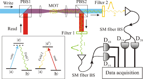
Figure 1: Schematic of experiment for conditional generation of single photons. Write and read pulses sequentially propagate into a cloud of cold Cs atoms (MOT), generating the correlated output fields $(1,2)$. A detection event for field $1$ at $D_{1A,1B}$ leads to an approximate one-photon state for field $2$, as confirmed with detectors $D_{2A,2B}$. (P)BS - (polarization) beam splitter, SM - single-mode. The inset illustrates the relevant atomic level scheme.

Inspired by the protocol of Ref. duan01 , in this Letter we report a significant advance in the creation of single photons for diverse applications in quantum information science, namely the generation and storage of single quanta from an atomic ensemble. As illustrated in Figure 1, an initial write pulse of (classical) light creates a state of collective excitation in an ensemble of cold atoms as determined by photoelectric detection for the generated field $1$. Although this first step is probabilistic, its success heralds the preparation of one excitation stored within the atomic medium. After a programmable delay $\delta t$, a read pulse converts the state of atomic excitation into a field excitation, thereby generating one photon in a well-defined spatial and temporal mode $2$. The quantum character of the $(1,2)$ fields is demonstrated by the observed violation of a Cauchy-Schwarz inequality for the ratio $R$ of cross correlations to auto-correlations clauser74 , namely $R=53\pm 2$ where $R\leq 1$ for any classical field kuzmich03 ; jiang03 ; kuzmich03-si .

This greatly improved nonclassical correlation for photon pairs for the $(1,2)$ fields enables the conditional generation of single photons as in Refs. grangier86 ; hong86 ; schiller01 ; pitman02 ; altepeter03 ; uren03 , but now with the photon $2$ stored as an excitation in the atomic ensemble pitman02 . Given a first photon $1$ from the write pulse, we trigger the emission of a second photon $2$ with the read pulse. To demonstrate the single-photon character of the field $2$, we measure the three-fold correlation function $w(1_{2},1_{2}|1_{1})$ for detection of two photons $(1_{2},1_{2})$ from field $2$ given a detection event $1_{1}$ from field $1$, where $w(1_{2},1_{2}|1_{1})=1$ for coherent states and $w(1_{2},1_{2}|1_{1})\geq 1$ for any classical field. Experimentally, we find $w(1_{2},1_{2}|1_{1})=0.34\pm 0.06$ for $\delta t=150$ ns, while $w(1_{2},1_{2}|1_{1})=0.24\pm 0.05$ for $\delta t=0$, thereby taking an important step toward the creation of ideal single photons for which $w(1_{2},1_{2}|1_{1})\rightarrow 0$.

Figure 1 provides an overview of our experiment for producing correlated photons from an optically thick sample of four-level atoms in a magneto-optical trap (MOT) kuzmich03 ; metcalf99 . The ground states $\{|a\rangle;|b\rangle\}$ correspond to the $6S_{1/2},F=\{4;3\}$ levels in atomic Cs, while the excited states $\{|e\rangle;|e^{\prime}\rangle\}$ denote the $\{6P_{3/2},F=4;6P_{1/2},F=4\}$ levels of the $D_{2},D_{1}$ lines at $\{852;894\}$ nm, respectively. We start the protocol for single photon generation by shutting off all light responsible for trapping and cooling for $1\mu$s, with the trapping light turned off approximately $300$ ns before the re-pumping light in order to empty the $F=3$ hyperfine level in the Cs $6S_{1/2}$ ground state, thus preparing the atoms in $|a\rangle$. During the “dark” period, the $j^{\text{th}}$ trial is initiated at time $t_{j}^{(1)}$ when a rectangular pulse of laser light from the write beam, $150$ ns in duration (FWHM) and tuned $10$ MHz below the $|a\rangle\rightarrow|e\rangle$ transition, induces spontaneous Raman scattering to level $|b\rangle$ via $|a\rangle\rightarrow|e\rangle\rightarrow|b\rangle$. The write pulse is sufficiently weak so that the probability to scatter one Raman photon into a forward propagating wavepacket $\psi^{(1)}(\vec{r},t_{j}^{(1)})$ is less than unity for each pulse. Detection of one photon from field $1$ results in a “spin” excitation to level $|b\rangle$, with this excitation distributed in a symmetrized, coherent manner throughout the sample of $N$ atoms illuminated by the write beam.

Given this initial detection, the stored atomic excitation can be converted into one quantum of light at a user controlled time $t_{j}^{(2)}=t_{j}^{(1)}+\delta t$. To implement this conversion, a rectangular pulse from the read beam, $120$ ns in duration (FWHM) and resonant with the $|b\rangle\rightarrow|e^{\prime}\rangle$ transition, illuminates the atomic sample. This pulse affects the transfer $|b\rangle\rightarrow|e^{\prime}\rangle\rightarrow|a\rangle$ with the accompanying emission of a second Raman photon $2$ on the $|e^{\prime}\rangle\rightarrow|a\rangle$ transition described by the wavepacket $\psi^{(2)}(\vec{r},t_{j}^{(2)})$, where the spatial and temporal structure of $\psi^{(1,2)}(\vec{r},t)$ are discussed in more detail in Ref. duan02 . The trapping and re-pumping light for the MOT are then turned back on to prepare the atoms for the next trial $j+1$, with the whole process repeated at $250$ kHz.

The forward-scattered Raman light from the write, read pulses is directed to two sets of single-photon detectors ($D_{1A,1B}$ for field $1$ and $D_{2A,2B}$ for field $2$) qe . Light from the (write, read) pulses is strongly attenuated (by $\simeq 10^{6}$) by the filters shown in Fig. 1, while the associated $(1,2)$ photons from Raman scattering are transmitted with high efficiency ($\simeq 80\%$) kuzmich03 . Detection events from $D_{1A,1B}$ within the intervals $[t_{j}^{(1)},t_{j}^{(1)}+T]$ and from $D_{2A,2B}$ within $[t_{j}^{(2)},t_{j}^{(2)}+T]$ are time stamped (with a resolution of $2$ ns) and stored for later analysis. $T=200$ ns for all of our measurements.

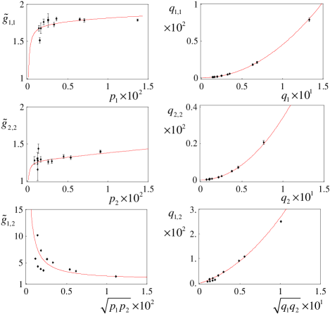
Figure 2: Left column (a) – (c) Normalized intensity correlation functions $\tilde{g}_{1,1},\tilde{g}_{2,2},\tilde{g}_{1,2}$ versus observed detection probabilities $p_{1},p_{2},\sqrt{p_{1}p_{2}}$, respectively. Right column (d) – (f) $q_{1,1},q_{2,2},q_{1,2}$ for joint detection versus $q_{1},q_{2},\sqrt{q_{1}q_{2}}$ for single detection, with $q_{l},q_{l,m}$ referenced to the output of the MOT. Statistical uncertainties are indicated by the error bars. The full curves are from the model calculation described in the text with $(\kappa_{1},\kappa_{2})=(0.17,0.90)$ and $(|v_{1b}|^{2},|v_{2b}|^{2})=0.006$.

For a particular set of operating conditions, we determine the single $p_{l}$ and joint $p_{l,m}$ event probabilities from the record of detection events at $D_{1A,1B},D_{2A,2B}$, where $(l,m)=1$ or $2$. For example, the total singles probability $p_{1}$ for events at $D_{1A},D_{1B}$ due to field $1$ is found from the total number of detection events $n_{1A}+n_{1B}$ recorded by $D_{1A},D_{1B}$ during the intervals $[t_{j}^{(1)},t_{j}^{(1)}+T]$ over $M_{tot}$ repeated trials $\{j\}$, with then $p_{1}=(n_{1A}+n_{1B})/M_{tot}$. To determine $p_{1,1}$ for joint detections at $D_{1A},D_{1B}$, we count the total number of coincidences $N_{1A,1B}$ recorded by $D_{1A},D_{1B}$, with then $p_{1,1}=N_{1A,1B}/M_{tot}$. $p_{2,2}$ is found in an analogous fashion using events from $D_{2A},D_{2B}$. Joint detections between the $(1,2)$ fields are described by $p_{1,2}$, which is determined by summing coincidence events between the four pairs of detectors for the $(1,2)$ fields (e.g., between pairs $D_{1A},D_{2A}$).

From $(p_{l},p_{l,m})$ we derive estimates of the normalized intensity correlation functions $\tilde{g}_{l,m}$, where $\tilde{g}_{l,m}=1$ for coherent states. For example, the auto-correlation function $\tilde{g}_{1,1}=p_{1,1}/(p_{1A}p_{1B})$ for field $1$, and similarly for the functions $\tilde{g}_{2,2},\tilde{g}_{1,2}$ for the auto-correlation of field $2$ and the cross correlation between fields $(1,2)$. The first column in Figure 2 displays $\tilde{g}_{1,1},\tilde{g}_{2,2}$, and $\tilde{g}_{1,2}$ as functions of $p_{1},p_{2},$ and $\sqrt{p_{1}p_{2}}$ consistency . A virtue of $\tilde{g}_{l,m}$ is its independence from the propagation and detection efficiencies. In the ideal case, the state for the fields $(1,2)$ is duan01 ; duan02 ; kuzmich03-si

$$|\Phi_{12}\rangle=|00\rangle+\sqrt{\chi}|11\rangle+\chi|22\rangle+O(\chi^{3/2})\text{ ,}$$ (1)

where $\sqrt{\chi}$ is the excitation amplitude for field $1$ in each trial of the experiment. For $\chi\ll 1$, $\tilde{g}_{1,1}=\tilde{g}_{2,2}\simeq 2$ and $\tilde{g}_{1,2}=1+1/\chi$. By contrast, for reasons that we will shortly address, our measurements in Fig. 2 give $\tilde{g}_{1,1}\simeq 1.7$ and $\tilde{g}_{2,2}\simeq 1.3$, with $\tilde{g}_{1,2}$ exhibiting a sharp rise with decreasing $\sqrt{p_{1}p_{2}}$, but with considerable scatter.

To provide a characterization of the field generation that is independent of the efficiency of our particular detection setup, we convert the photodetection probabilities $(p_{l},p_{l,m})$ to the quantities $(q_{l},q_{l,m})$ for the field mode collected by our imaging system at the output of the MOT. Explicitly, for single events for fields $(1,2)$, we define $q_{1}\equiv p_{1}/\alpha_{1},q_{2}\equiv p_{2}/\alpha_{2}$, while for joint events, $q_{1,1}\equiv p_{1,1}/\alpha_{1}^{2},q_{2,2}\equiv p_{2,2}/\alpha_{2}^{2},q_{1,2}\equiv p_{1,2}/\alpha_{1}\alpha_{2}$, where $\alpha_{l}$ gives the collection, propagation, and detection efficiency qe . The second column in Fig. 2 displays the measured dependence of $q_{l,m}$ for joint events versus $q_{1},q_{2},\sqrt{q_{1}q_{2}}$ for single events over a range of operating conditions. As expected from Eq. 1, $q_{1,1},q_{2,2}$ exhibit an approximately quadratic dependence on $q_{1},q_{2}$, while $q_{1,2}$ would be linear for $\sqrt{q_{1}q_{2}}\ll 1$ in the ideal case.

In our experiment there are a number of imperfections that lead to deviations from the ideal case expressed by $|\Phi_{12}\rangle$ duan01 ; kuzmich03-si ; duan02 . To capture the essential aspects, we have developed a simple model that assumes the total fields $(1,2)$ at the output of the MOT consist of contributions from $|\Phi_{12}\rangle$, together with background fields in coherent states $|v_{1,2}\rangle$. Operationally, increases in $p_{1},p_{2}$ are accomplished by way of increases in the intensity of the write beam, with only minor adjustments to the read beam. Hence, we parameterize our model by taking $\chi=|v_{w}|^{2}$, with $v_{w}$ as the (scaled) amplitude of the write beam. Since important sources of noise are light scattering from the write and read beams and background fluorescence from uncorrelated atoms in the sample duan02 , we assume that $v_{1,2}=\sqrt{\kappa_{1,2}}v_{w}$. We further allow for fixed incoherent backgrounds $v_{1b},v_{2b}$ to account for processes that do not depend upon increases in the write intensity.

With this model, it is straightforward to compute the quantities that appear in Figs. 2–4. The parameters $(\kappa_{1},\kappa_{2})=(0.17,0.90)$ and $(|v_{1b}|^{2},|v_{2b}|^{2})=0.006$ are obtained directly by optimizing the comparison between the model results and our measurements of normalized correlation functions (e.g., $\tilde{g}_{1,1}$ vs. $\tilde{g}_{1,2}$) without requiring absolute efficiencies. $\kappa_{1}=0.17$ implies that the photon number for “good” events associated with $|\Phi_{12}\rangle$ exceeds that for “bad” (background) events from $|v_{1}\rangle$ by roughly $6-$fold for detection at $D_{1A},D_{1B}$. For the curves in Fig. 2, we must also obtain the efficiencies $\beta_{l},\eta_{l}$ that convert expectation values for normally ordered photon number operators $\hat{n}_{l}$ for fields $l=(1,2)$ in the model into the various $(p_{l},p_{l,m})$ and $(q_{l},q_{l,m})$ (e.g., $p_{l}=\beta_{l}\langle\hat{n}_{l}\rangle,q_{l}=\eta_{l}\langle\hat{n}_{l}\rangle,q_{1,2}=\eta_{1}\eta_{2}\langle\colon\hat{n}_{1}\hat{n}_{2}\colon\rangle$). Ideally $\beta_{l}=\alpha_{l}$ and $\eta_{l}=1$; we find instead $(\beta_{l},\eta_{l})=(0.013,0.15)$, where we take $\beta_{1}=\beta_{2}$ and $\eta_{1}=\eta_{2}$ for simplicity. Among various candidates under investigation, values $\beta_{l}<\alpha_{l},\eta_{l}<1$ can arise from inherent mode mismatching for capturing collective emission from the atomic ensemble duan02 .

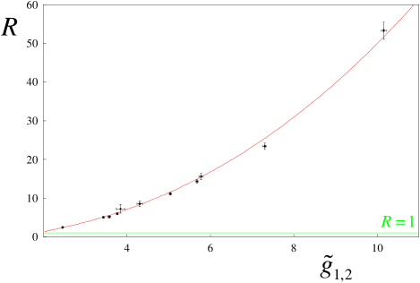
Figure 3: Ratio $R\equiv\left[\tilde{g}_{1,2}\right]^{2}/\tilde{g}_{1,1}\tilde{g}_{22}$ versus the normalized cross correlation $\tilde{g}_{1,2}$, where $R>1$ for manifestly quantum (nonclassical) fields. The points are from our experiment with statistical uncertainties indicated by the error bars. The full curve is from the model calculation with $(\kappa_{1},\kappa_{2})$ and $(|v_{1b}|^{2},|v_{2b}|^{2})$ as in Fig. 2.

Independent of the absolute efficiencies, we can utilize the results from Fig. 2 to address directly the question of the nonclassical character of the $(1,2)$ fields by following the pioneering work of Clauser clauser74 . The correlation functions $\tilde{g}_{l,m}$ for fields for which the Glauber-Sudarshan phase-space function $\varphi$ is well-behaved (i.e., classical fields) are constrained by the inequality $R\equiv\left[\tilde{g}_{1,2}\right]^{2}/\tilde{g}_{1,1}\tilde{g}_{2,2}\leq 1$ clauser74 ; kuzmich03-si . In Fig. 3 we plot the experimentally derived values for $R$ as a function of the degree of cross-correlation $\tilde{g}_{1,2}$ consistency . As compared to previous measurements for which $R=1.84\pm 0.06$ kuzmich03 and $R=1.34\pm 0.05$ jiang03 , we have now achieved $R\gg 1$, with $R=53\pm 2$ for the largest value of $\tilde{g}_{1,2}$. In Figs. 2 and 3 as well as 4 to follow, all points are taken with $\delta t=150$ ns, except the points at $\tilde{g}_{1,2}\simeq 10$, which have $\delta t=0$.

This large degree of quantum correlation between the $(1,2)$ fields suggests the possibility of producing a single photon for field $2$ by conditional detection of field $1$. To investigate this possibility, we consider the three-fold correlation function $w(1_{2},1_{2}|1_{1})$ for detection with the setup shown in Fig. 1, namely

$$w(1_{2},1_{2}|1_{1})\equiv\frac{p^{(c)}(1_{2},1_{2}|1_{1})}{[p^{(c)}(1_{2}|1_{1})]^{2}}\text{, }$$ (2)

where $p^{(c)}(1_{2},1_{2}|1_{1})$ is the conditional probability for detection of two photons $(1_{2},1_{2})$ from field $2$ conditioned upon the detection of an initial photon $1_{1}$ for field $1$, and $p^{(c)}(1_{2}|1_{1})$ is the probability for detection of one photon $1_{2}$ given a detection event $1_{1}$ for field $1$. Bayes’ theorem allows the conditional probabilities in Eq. 2 to be written in terms of single and joint probabilities $p^{(k)}$ for $k-$fold detection, so that

$$w(1_{2},1_{2}|1_{1})=\frac{p^{(1)}(1_{1})p^{(3)}(1_{1},1_{2},1_{2})}{[p^{(2)}(1_{1},1_{2})]^{2}}\text{.}$$ (3)

Fields with a positive-definite $\varphi$ must satisfy the Cauchy-Schwarz inequality $w(1_{2},1_{2}|1_{1})\geq 1$. Indeed, for independent coherent states, $w=1$, while for thermal beams, $w=2$. By contrast, for the state $|\Phi_{12}\rangle$ of Eq. 1, $w=4\chi\ll 1$ for small $\chi$, approaching the ideal case $w\rightarrow 0$ for a “twin” Fock state $|1_{1}1_{2}\rangle$.

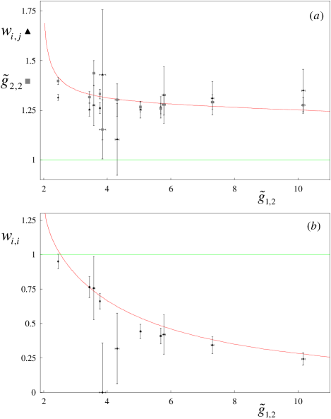
Figure 4: Three-fold correlation function $w(1_{2},1_{2}|1_{1})$ for detection event $1_{1}$ for field $1$ followed by two events $(1_{2},1_{2})$ for field $2$ versus the normalized cross correlation $\tilde{g}_{1,2}$. (a) $w_{i,j}(1_{2},1_{2}|1_{1})$ for events $(1_{1})_{i}$ and $(1_{2},1_{2})_{j}$ from different trials $i\neq j$ together with points for $\tilde{g}_{2,2}$. $w_{i,j}=\tilde{g}_{2,2}$ for statistically independent trials. (b) $w_{i,i}(1_{2},1_{2}|1_{1})$ for events from the same trial $i$. $w_{i,i}<1$ for sub-Poissonian fields in support of the single-photon character of field $2$. Statistical uncertainties are indicated by the error bars. The full curves are from the model calculation with $(\kappa_{1},\kappa_{2})$ and $(|v_{1b}|^{2},|v_{2b}|^{2})$ as in Figs. 2, 3.

From the record of photo-detection events at $D_{1A,1B},D_{2A,2B}$, we calculate estimates of the various probabilities appearing in Eq. 3, with the results of this analysis shown in Fig. 4. Part (a) examines the quantity $w_{i,j}(1_{2},1_{2}|1_{1})$ obtained from events taken from different trials $i\neq j$ for the $(1,2)$ fields (i.e., detection $1_{1}$ in trial $i$ for field $1$ followed by two detections $(1_{2},1_{2})$ in trial $j$ for field $2$). In this case, the $(1,2)$ fields should be statistically independent kuzmich03-si , so that $w_{i,j}(1_{2},1_{2}|1_{1})=\tilde{g}_{2,2}$. Hence, we also superimpose $\tilde{g}_{2,2}$ from Fig. 2 and find reasonable correspondence within the statistical uncertainties (in particular, $w_{i,j}(1_{2},1_{2}|1_{1})\gtrsim 1$), thereby validating our analysis techniques consistency . No corrections for dark counts or other backgrounds have been applied to the data in Fig. 4 (nor indeed to Figs. 2, 3).

Fig. 4 (b) displays $w_{i,i}(1_{2},1_{2}|1_{1})$ for events from the same experimental trial $i$ for the $(1,2)$ fields. Significantly, as the degree of cross-correlation expressed by $\tilde{g}_{1,2}$ increases (i.e., decreasing $\chi$), $w_{i,i}(1_{2},1_{2}|1_{1})$ drops below the classical level of unity, indicative of the sub-Poissonian character of the conditional state of field $2$. For $\delta t=150$ ns, $w_{i,i}(1_{2},1_{2}|1_{1})=0.34\pm 0.06$ for $\tilde{g}_{1,2}=7.3$, while with $\delta t=0$, $w_{i,i}(1_{2},1_{2}|1_{1})=0.24\pm 0.05$ for $\tilde{g}_{1,2}=10.2$. Beyond the comparison to our model shown the figure, empirically we find that $w_{i,i}(1_{2},1_{2}|1_{1})$ is well approximated by $\tilde{g}_{1,1}\tilde{g}_{2,2}/\tilde{g}_{1,2}$, as in the ideal case of Eq. 1. However, independent of such comparisons, we stress that the observations reported in Fig. 4 represent a sizable nonclassical effect in support of the conditional generation of single photons for field $2$.

In conclusion, our experiment represents an important step in the creation of an efficient source of single photons stored within an atomic ensemble, and thereby towards enabling diverse protocols in quantum information science knill01 ; lutkenhaus00 ; duan01 ; duan03 . Our model supports the hypothesis that the inherent limiting behavior of $w_{i,i}(1_{2},1_{2}|1_{1})$ below unity is set by the efficiency $\eta_{l}$, which leads to prohibitively long times for data acquisition for $\chi\lesssim 0.04$, corresponding to the smallest value of $w_{i,i}$ in Fig. 4. We are pursuing improvements to push $\eta_{l}\simeq 0.15\rightarrow 1$, including in the intrinsic collection efficiency following the analysis of Ref. duan02 . Dephasing due to Larmor precession in the quadrupole field of the MOT limits $\delta t\lesssim 300$ ns, which can be extended to several seconds in optical dipole or magnetic traps metcalf99 .

We gratefully acknowledge the contributions of A. Boca, D. Boozer, W. Bowen, and L.-M. Duan. This work is supported by ARDA, and by the Caltech MURI Center for Quantum Networks and by the NSF.

^∗ School of Physics, Georgia Institute of Technology, Atlanta, Georgia 30332

References

- (1) I. L. Chuang and Y. Yamamoto, Phys. Rev. A 52, 3489 (1995).
- (2) Q. A. Turchette et al., Phys. Rev. Lett. 75, 4710-4713 (1995).
- (3) E. Knill, R. Laflamme, and G. Milburn, Nature 409, 46-52 (2001).
- (4) N. Lutkenhaus, Phys. Rev. A 61, 052304 (2000).
- (5) H.-J. Briegel and S. J. van Enk, in The Physics of Quantum Information, eds. D. Bouwmeester, A. Ekert, and A. Zeilinger (Springer-Verlag, Berlin, 2000), 6.2 & 8.6.
- (6) L.-M. Duan, et al., Nature 414, 413 (2001).
- (7) L.-M. Duan and H. J. Kimble, quant-ph/0309187.
- (8) P. Michler et al., Science 290, 2282 (2000).
- (9) E. Moreau et al., Appl. Phys. Lett. 79, 2865 (2001).
- (10) M. Pelton et al., Phys. Rev. Lett. 89, 233602 (2002).
- (11) J. F. Clauser, Phys. Rev. D 9, 853 (1974).
- (12) P. Grangier, G. Roger, and A. Aspect, Europhys. Lett. 1, 173 (1986).
- (13) C. K. Hong and L. Mandel, Phys. Rev. Lett. 56, 58 (1986).
- (14) A. I. Lvovsky et al., Phys. Rev. Lett. 87, 050402 (2001).
- (15) T. B. Pittman, B. C. Jacobs, J. D. Franson, Phys. Rev. A66, 042303 (2002).
- (16) J. B. Altepeter et al., Phys. Rev. Lett. 90, 193601 (2003).
- (17) A. B. U’Ren et al., quant-ph/0312118.
- (18) B. Julsgaard et al., Q. Inf. & Computation 3, 518 (2003).
- (19) M. Lukin, Rev. Mod. Phys. 75, 457 (2003).
- (20) A. Kuzmich et al., Nature 423, 731 (2003).
- (21) Wei Jiang et al., quant-ph/0309175.
- (22) See Supplementary Information accompanying Ref. kuzmich03 .
- (23) Laser Cooling and Trapping, H. J. Metcalf and P. van der Straten (Springer-Verlag, 1999).
- (24) L.-M. Duan, J. I. Cirac, and P. Zoller, Phys. Rev. A 66, 023818 (2002).
- (25) As a consistency check, we have employed white light for measurements as in Figs. , and find that , where in all cases, these correlation functions should equal unity.
- (26) The overall efficiencies , where for light with the spatial shape of the write, read beams propagating from the MOT to the input beam splitters for detectors , which have quantum efficiencies (i.e., photon in to TTL pulse out). The efficiencies for PBS2 in Fig. 1 account for the presumed unpolarized character of the fields in our experiment.