Luttinger liquid of polarons in one-dimensional boson-fermion mixtures

Abstract

We use bosonization approach to investigate quantum phases in mixtures of bosonic and fermionic atoms confined in one dimensional optical lattices. The phase diagrams can be well understood in terms of polarons, which correspond to atoms that are ”dressed” by screening clouds of the other atom species. For a mixture of single species of fermionic and bosonic atoms we find a charge density wave phase, a phase with fermion pairing, and a regime of phase separation. For a mixture of two species of fermionic atoms and one species of bosonic atoms we obtain spin and charge density wave phases, a Wigner crystal phase, singlet and triplet paired states of fermions, and a phase separation regime. Equivalence between the Luttinger liquid description of polarons and the canonical polaron transformation is established and the techniques to detect the resulting quantum phases are discussed.

Mixtures of ultra-cold bosonic and fermionic atoms, that have recently become accessible experimentally, represent a promising new system for studying strongly correlated many-body physics bfm . Bosonic atoms mediate interactions between fermions and allow efficient cooling of the system sympathetic_cooling . Several novel phenomena have been predicted theoretically for Boson-Fermion mixtures (BFM) including pairing of fermions pairing , formation of composite particles composite , spontaneous breaking of translational symmetry in optical lattices burnett and appearance of charge density wave (CDW) xCDW . Most of these theoretical studies relied on integrating out bosonic degrees of freedom to obtain an effective interaction between fermions, and then using a mean-field approach to investigate many-body states pairing . This approach, however, becomes unreliable in the regime of strong interactions. In particular, it fails in low-dimensional systems due to enhanced fluctuations and non-perturbative effects of interactions.

In this paper we use bosonization method haldane_bf ; cazalilla to investigate one dimensional (1D) BFM. The resulting quantum phases can be understood by introducing polarons, i.e. atoms of one species surrounded by screening clouds of the other species. Such dressed quasi-particles exhibit effective interactions and modified effective masses. In our analysis the polarons emerge as quasi-particles with the slowest decaying correlation functions while quantum phases of the system arise from a competition of various ordering instabilities of such polarons. The phase diagrams we obtain (Figs. 1-3) show a remarkable similarity to the Luttinger liquid phase diagrams of 1D interacting electron systems solyom , suggesting that 1D BFM may be understood as Luttinger liquids of polarons.

In Fig. 1 we show a phase diagram for a mixture of bosons and spinless fermions as a function of experimentally controlled parameters: the scattering length between bosons and fermions ($a_{bf}$) and the strength of the longitudinal optical lattice for bosonic atoms ($V_{b,\|}$) endnote1 .

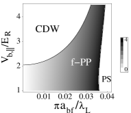
Figure 1: Phase diagram for a mixture of bosonic and spinless fermionic atoms in a 1D optical lattice. Shading in the $f$-PP phase describes the strength of the bosonic screening cloud ($2\lambda$, see Eq.(9)) around a pair of fermions. $\lambda_{L}$ and $E_{R}$ are respectively the lattice period and recoil energy. Other parameters used for this figure are (see text for notations): $\nu_{b}=4$, $\nu_{f}=0.5$, $V_{b,\perp}=V_{f,\perp}=20E_{R}$, $V_{f,\|}=2E_{R}$, boson-boson scattering length $a_{bb}=0.01\lambda_{L}$.

For relatively weak boson-fermion interactions and slow bosons (i.e. strong optical lattice for bosonic atoms) the system is in the CDW phase, in which the densities of fermions and bosons have a $2k_{f}$-modulation. In the case of very strong boson-fermion interactions the system is unstable to phase separation (PS) ho ; instability . The two regimes are separated by a p-wave pairing phase of fermionic polarons ($f$-PP). While we carry out the detailed analysis for atoms in optical lattices, qualitatively it also applies to the continuous case bfm ; sympathetic_cooling ; general_1D .

Before proceeding we note that bosonization approach has been applied to BFM in Ref.[ho, ]. However this work did not consider correlations of polaronic degrees of freedom, and as a result did not predict most of the quantum phases. The present system also resembles 1D electron-phonon systems discussed previously in Ref.[voit_phonon, ]. The key difference between the two is that the sound velocity in a solid state is typically smaller than the Fermi velocity, whereas for the dilute fermionic gas coupled to superfluid bosonic ensemble the opposite is true. In particular, this rules out an adiabatic elimination of the bosonic field. In contrast, we demonstrate in the present system polaronic quasi-particles dominate the low-temperature behaviour of the system. We also note that the 1-D $p$-wave superfluid we obtain here may be of relevance to recent studies in quantum information in Ref.[kitaev, ].

We first consider a mixture of spinless fermionic ($f$) and bosonic ($b$) atoms. For sufficiently strong optical potential the microscopic Hamiltonian is given by a single band Hubbard model

$$H = -\sum_{\langle ij\rangle}\left(t_{b}b_{i}^{\dagger}b_{j}+t_{f}f_{i}^{\dagger}f_{j}\right)-\sum_{i}\left(\mu_{f}n_{f,i}+\mu_{b}n_{b,i}\right)$$ (1)

$$+\frac{U_{b}}{2}\sum_{i}n_{b,i}(n_{b,i}-1)+U_{bf}\sum_{i}n_{b,i}n_{f,i},$$

Here $n_{b,i}\equiv b^{\dagger}_{i}b_{i}$ and $n_{f,i}\equiv f^{\dagger}_{i}f_{i}$ are respectively the boson and fermion density operators, and $\mu_{b/f}$ are their chemical potentials. The tunneling amplitudes $t_{f/b}$, and the particle interactions $U_{b}$ and $U_{bf}$ depend on the laser beam intensities and the $s$-wave scattering lengths, and can be calculated explicitly (see e.g. Ref.[Jaksch98, ]). In this paper we assume that the filling fraction of fermions $\nu_{f}\equiv\langle n_{f,i}\rangle$ is not commensurate with the lattice or with the filling fraction of bosons $\nu_{b}$. The Fermi momentum and velocity are given by $k_{f}=\pi\nu_{f}$ and $v_{f}=2t_{f}\sin(k_{f})$,respectively.

The Haldane’s bosonization representations for fermion and boson operators are constructed as haldane_bf ; ho $f(x)=\left[\nu_{f}+\Pi_{f}\right]^{1/2}\sum_{m=-\infty}^{\infty}e^{(2m+1)i\Theta_{f}}e^{i\Phi_{f}}$ and $b(x)=\left[\nu_{b}+\Pi_{b}\right]^{1/2}\sum_{m=-\infty}^{\infty}e^{2mi\Theta_{b}}e^{i\Phi_{b}}$, where $x$ is a continuous coordinate that replaces the site index $i$ in Eq. (1). The operators $\Pi_{f/b}(x)$ and $\Phi_{f/b}(x)$ describe the bosonized density and phase operators for each of the atomic species, and satisfy the commutation relations $\left[\Pi_{b/f}(x),\Phi_{b/f}(x^{\prime})\right]=i\delta(x-x^{\prime})$. Short-ranged fluctuations are taken into account via the harmonics of $\Theta_{f/b}(x)=\pi\nu_{f/b}x+\pi\int^{x}dy\,\Pi_{f/b}(y)$. The low energy effective Hamiltonian can be written to be the sum of the following terms:

$$H_{f}^{0} = \frac{v_{f}}{2}\int_{0}^{L}dx\left[\frac{1}{\pi}\left(\partial_{x}\Phi_{f}(x)\right)^{2}+\pi\Pi_{f}(x)^{2}\right]$$ (2)

$$H_{b}^{0} = \frac{v_{b}}{2}\int_{0}^{L}dx\left[\frac{K_{b}}{\pi}\left(\partial_{x}\Phi_{b}(x)\right)^{2}+\frac{\pi}{K_{b}}\Pi_{b}(x)^{2}\right]$$ (3)

$$H^{1}_{bf} = U_{bf}\int_{0}^{L}dx\,\Pi_{b}(x)\Pi_{f}(x)$$ (4)

$$H^{2}_{bf} = U_{bf}\int_{0}^{L}dx\,\Pi_{b}(x)\tilde{n}_{f}(x),$$ (5)

where we neglected the Umklapp scattering and backward scattering of bosons by assuming that bosons are deep inside the superfluid regime halffilling . When the boson-boson interaction is weak (i.e. $\gamma\equiv m^{\ast}_{b}U_{b}/\nu_{s}<10$), the phonon velocity $v_{b}$ and the scaling exponent of bosons $K_{b}$ in Eq.(3) can be well approximated by $v_{b}=\frac{\nu_{s}}{m^{\ast}_{b}}\sqrt{\gamma}\left(1-\frac{\sqrt{\gamma}}{2\pi}\right)^{1/2}$ and $K_{b}=\frac{\pi}{\sqrt{\gamma}}\left(1-\frac{\sqrt{\gamma}}{2\pi}\right)^{-1/2}$, where $m^{\ast}_{b}$ is the effective boson mass in the presence of the lattice potential stringari and $\nu_{s}\sim\nu_{b}$ is the superfluid fraction. The term $H_{bf}^{1}$ in Eq. (4) describes forward scattering between bosons and fermions, and the term $H_{bf}^{2}$ corresponds to back scattering of fermions on bosons (We defined $\tilde{n}_{f}(x)=\frac{1}{L}\sum_{k\sim 2k_{f}}\sum_{p\sim k_{f}}\left[e^{ikx}f^{\dagger}_{R,-p+k}f_{L,-p}+e^{-ikx}f^{\dagger}_{L,p-k}f_{R,p}\right]$, where $f_{\{R,L\},p}^{\dagger}$ are the creation operators for the right and left moving fermions near the Fermi energy). It is useful, however, to take into account the deviations of the phonon dispersion from the linear spectrum by using the Bogoliubov approximation $\omega_{k}=\sqrt{(\varepsilon_{b,k}-\varepsilon_{b,0})(\varepsilon_{b,k}-\varepsilon_{b,0}+2U_{b}\nu_{b})}$, where $\varepsilon_{b,k}$ is the band energy of a noninteracting boson.

We integrate out the $2k_{f}$-bosons and obtain an effective fermion-fermion interaction. Since we are considering a BFM with fast phonon velocity, i. e. $v_{b}\gg v_{f}$, we obtain within instantaneous approximation:

$$H_{f}^{1} = \frac{2G}{2\pi}\int_{0}^{L}dx\left[\pi^{2}\Pi_{f}(x)^{2}-(\partial_{x}\Phi_{f}(x))^{2}\right].$$ (6)

Here $G\equiv\frac{g_{2k_{f}}^{2}}{\omega_{2k_{f}}}$ is the induced fermion-fermion interaction, and $g_{k}$ is the fermion-phonon (FP) coupling vertex, $g_{k}=U_{bf}\sqrt{\nu_{b}(\varepsilon_{b,k}-\varepsilon_{b,0})/2\pi\omega_{k}}$. Note, that for small $k$ we have a conventional FP coupling $g_{k}=g|k|^{1/2}$ with $g=U_{bf}\sqrt{K_{b}}/2\pi$. Therefore the effective Hamiltonian for a BFM is given by Eqs. (2)-(4) and (6) with five parameters: $v_{f}$, $v_{b}$, $K_{b}$, $g$ and $G$. We can diagonalize this Hamiltonian Engelsberg and obtain

$$H = \frac{1}{2}\sum_{j=a,A}v_{j}\int dx\left[\pi\Pi_{j}(x)^{2}+\frac{1}{\pi}\left(\partial_{x}\Phi_{j}(x)\right)^{2}\right]$$ (7)

where the eigenmode velocities, $v_{A}$ and $v_{a}$, are given by

$$v_{a/A}^{2} = \frac{1}{2}(v_{b}^{2}+\tilde{v}_{f}^{2})\pm\frac{1}{2}\sqrt{(v_{b}^{2}-\tilde{v}_{f}^{2})^{2}+16\tilde{g}^{2}v_{b}\tilde{v}_{f}}.$$ (8)

Here $\tilde{v}_{f}\equiv(v_{f}^{2}-4G)^{1/2}$ and $\tilde{g}\equiv g\,e^{\theta}$ with $e^{\theta}=((v_{f}-2G)/(v_{f}+2G))^{1/4}$.

When the FP coupling $g$ becomes sufficiently strong, the eigenmode velocity $v_{A}$ becomes soft, indicating an instability of the system to phase separation or collapse, depending on the sign of $U_{bf}$ ho ; instability . To understand the nature of the many-body state of BFM outside of the instability region we analyze the long distance behavior of the correlation functions. For the bare bosonic and fermionic particles we find $\langle b(x)b^{\dagger}(0)\rangle\sim|x|^{-\frac{1}{2}K_{\epsilon}^{-1}}$ and $\langle f(x)f^{\dagger}(0)\rangle\sim\cos(k_{f}x)|x|^{-\frac{1}{2}(K_{\beta}+K_{\gamma}^{-1})}$ (see Ref.[Definitions, ]). To describe particles dressed by the other species we introduce the composite operators

$$\tilde{f}_{\lambda}(x)\equiv e^{-i\lambda\Phi_{b}(x)}f(x),\ \ \ \tilde{b}_{\eta}(x)\equiv e^{-i\eta\Phi_{f}(x)}b(x),$$ (9)

with $\lambda$ and $\eta$ being real numbers. The correlation functions of these operators are given by $\langle\tilde{f}(x)\tilde{f}^{\dagger}(0)\rangle\sim\cos(k_{f}x)|x|^{-\frac{1}{2}(K_{\beta}+\lambda^{2}K_{\epsilon}^{-1}+K_{\gamma}^{-1}-2\lambda K_{\gamma\epsilon}^{-1})}$ and $\langle\tilde{b}(x)\tilde{b}^{\dagger}(0)\rangle\sim|x|^{-\frac{1}{2}(K_{\epsilon}^{-1}+\eta^{2}K_{\gamma}^{-1}-2\eta K_{\gamma\epsilon}^{-1})}$ (see Ref.[Definitions, ]). We observe that the exponents of the correlation functions are maximized with $\lambda_{c}=K_{\epsilon}/K_{\gamma\epsilon}$ and $\eta_{c}=K_{\gamma}/K_{\gamma\epsilon}$, which we use to construct polaronic particles according to Eq. [9]. In the limit of weak interactions we have $\lambda_{c}\to U_{bf}/U_{b}$ and $\eta_{c}\to 2U_{bf}/\pi v_{b}$. This result can be understood by a naive density counting argument that a fermionic polaron ($f$-polaron) locally suppresses a bosonic cloud by $\lambda_{c}$ particles, whereas a bosonic polaron ($b$-polaron) depletes the fermionic system by $\eta_{c}$ atoms.

Ground states of one dimensional systems are often characterized by specifying the order parameters that have the slowest long distance decay of the correlation functions solyom . This is equivalent to finding the most divergent susceptibility in the low temperature limit (When the $T=0$ correlation function decays as $\langle O(x)O(0)\rangle\sim 1/|x|^{2-\alpha}$, the finite $T$ susceptibility diverges as $\chi(T)\sim 1/T^{\alpha}$). For the $2k_{f}$ CDW order parameter, $O_{CDW}=f^{\dagger}_{L}f_{R}$, we find $\alpha_{CDW}=2-2K_{\beta}$, and for the $f$-polaron pairing field, $O_{f-PP}=\tilde{f}_{L\lambda}\tilde{f}_{R\lambda}$, we obtain $\alpha_{f-PP}=2-2\left[\lambda^{2}K_{\epsilon}^{-1}+K_{\gamma}^{-1}-2\lambda K_{\gamma\epsilon}^{-1}\right]$. We did not include polaron dressing in $O_{CDW}$, since this operator has no net fermionic charge and the exponent of $O_{CDW}$ does not change if we replace $f$ by $\tilde{f}$. For the $f$-PP operator, on the other hand, $\alpha_{f-PP}$ is maximized when $\lambda=\lambda_{c}$, so from now on $\alpha_{f-PP}$ will always mean the $f$-PP exponent computed with the optimal $\lambda_{c}$. Scaling exponents shown in Fig. 2(a) demonstrate that divergencies of the CDW and $f$-PP susceptibilities are mutually exclusive and cover the entire phase diagram. In Fig. 2(b) we show a global phase diagram of a BFM considering the FP coupling ($g$) and effective fermion-fermion interaction ($G$) as independent variables. This phase diagram is similar to what one finds for spinless electrons in Luttinger liquid theory solyom . The phase diagram in terms of experimentally controlled parameters was shown in Fig. 1. We point out that if we were to define the pairing operator using bare fermions rather than $f$-polarons with optimal $\lambda_{c}$, we would have a region in the phase diagram in which none of the susceptibilities diverges (for the parameters used in Fig. 2(a) this regime extends between $0.55<g/v_{f}<0.68$).

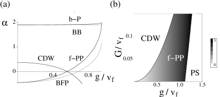
Figure 2: Ground state of a BFM with spinless fermions. $g$ is the longitudinal FP coupling and $G$ is the effective fermion-fermion interaction after integrating out $2k_{f}$ phonons. (a) Scaling exponents for $v_{b}/v_{f}=3$, $K_{b}=5$ and $G/v_{f}=0.1$. Different curves correspond to the $2k_{f}$ CDW order parameter, $f$-polaron pairing field ($f$-PP), bare fermion pairing field (BFP), $b$-polaron operator ($b$-P), and bare boson operator (BB). Note that operators constructed with polarons (bosons and Cooper pairs of fermions) always have larger exponents than their counterparts constructed with bare atoms. (b) Global phase diagram for $v_{b}/v_{f}=5$ and $K_{b}=10$.

We next verify that the conventional construction of polaron operators based on the canonical polaron transformation (CPT) mott can give an equivalent polaronic description as in Eq.[9]. The CPT operator is given by $U_{\lambda}=e^{-i\lambda\sum_{{k}\neq 0}\left(F_{k}\beta_{k}\rho_{k}^{\dagger}+{\rm h.c.}\right)}$, where $\beta_{k}$ is the phonon annihilation operator, $\rho_{k}$ is the fermion density operator, $F_{k}$ is some function of momentum ${k}$, and $\lambda$ specifies the strength of the phonon dressing. When applied to a fermion operator, the CPT gives $U^{-1}_{\lambda}f(x)U_{\lambda}=f(x)\exp\left[-i\lambda\sum_{{k}\neq 0}\left(F_{k}\beta_{k}e^{-i{k}\cdot{x}}+{\rm h.c.}\right)\right]$ mott , which is the same as Eq.(9), provided that one takes $F_{k}=\frac{1}{2}\sqrt{\frac{2\pi}{K_{b}|k|L}}{\rm sgn}(k)$ (note that in 1D fermionic systems density operators correspond to Luttinger bosons).

At finite temperature the correlation functions become $\langle O(x)O(0)\rangle\sim\exp(-|x|/\xi)/|x|^{2-\alpha}$. The thermal correlation lengths for $O_{CDW}$ and $O_{f-PP}$ are approximately given by $\xi\sim v_{f}/k_{B}T$. For a finite system of length $L=N\lambda_{L}$ ($N$ being the number of lattice sites), the $T=0$-properties of the system are visible for $\xi\sim L$. This corresponds to a temperature regime of $T\sim T_{f}/N$, $T_{f}$ being the Fermi temperature.

Before concluding our discussion of BFM with spinless fermions we discuss an approach for observing the phase transition between the CDW and the $f$-PP phases in laser stirring experiments stirring . Suppose that a laser beam is focused at the center of the cloud, such that it creates a weak local potential for fermionic atoms. In the $f$-PP phase the stirring potential can be moved through the system with no dissipation, if its velocity is slower than some critical value stirring . At the $f$-PP/CDW phase boundary the critical velocity goes to zero, reflecting a transition to the insulating (CDW) state. This scenario follows from an RG analysis of a small local potential for fermions: Such a potential is irrelevant in the $f$-PP phase, but becomes relevant in the CDW phase, similar to the single impurity problem of a 1D electron system kane . It should be emphasized that only when polarons are used to construct Cooper pairs, the paired phase coincides with the domain of irrelevance of a small pinning potential.

We now extend our analysis to BFM with fermions with two internal hyperfine states, which we assume to be $SU(2)$ symmetric. Spin symmetry of the system leads to separation of the bosonized Hamiltonian into spin and charge sectors. The charge part of the Hamiltonian is equivalent to a BFM with spinless atoms and can be diagonalized analogously. The spin part of the Hamiltonian has a form of the sine-Gordon model, $H_{\sigma}=\frac{1}{2}v_{\sigma}\int dx\left[\pi\Pi_{\sigma}(x)^{2}+\frac{1}{\pi}\left(\partial_{x}\Phi_{\sigma}(x)\right)^{2}\right]+\frac{2g_{1\perp}}{(2\pi\alpha)^{2}}\int dx\cos\left[\sqrt{8K_{\sigma}}\Theta_{\sigma}(x)\right],$ where $v_{\sigma}$ is the spin velocity, $K_{\sigma}$ is the spin Luttinger exponent, and $g_{1\perp}=U_{\uparrow\downarrow}-4\pi G$ is the effective backward scattering amplitude for fermions, that has contributions from the bare fermion-fermion interaction and from integrating out $2k_{f}$ phonons. The nature of spin excitations in the ground state follows from the well known properties of the sine-Gordon model: For $K_{\sigma}>1$ the system has gapless spin excitations ($g_{1\perp}$ is irrelevant), for $K_{\sigma}<1$ the system has a spin gap ($g_{1\perp}$ becomes relevant). In order to describe possible ground states of the system we calculated the low temperature behavior of susceptibilities for the following order parameters: $2k_{f}$ spin density wave ($\chi_{SDW}$), $2k_{f}$ charge density wave ($\chi_{CDW}$), $4k_{f}$ (Wigner crystal) charge density wave ($\chi_{WC}$), singlet polaron pairing ($\chi_{SPP}$), and triplet polaron pairing ($\chi_{TPP}$). Depending on the parameters we find the following regimes: 1) Equally divergent $\chi_{CDW}$ and $\chi_{SDW}$. Degenerate CDW and SDW phases; 2) Equally divergent $\chi_{SPP}$ and $\chi_{TPP}$. Degenerate SPP and TPP phases; 3) Divergent $\chi_{SPP}$. State with singlet pairing of polarons; 4) Both $\chi_{CDW}$ and $\chi_{SPP}$ diverge, but unequally. This probably corresponds to a phase that has both a CDW order and singlet polaron pairing; 5) Divergent $\chi_{CDW}$. CDW phase; 6) Divergent $\chi_{WC}$. Wigner crystal phase. The phase diagram in Fig. 3 again shows remarkable similarity to a phase diagram for interacting electrons solyom .

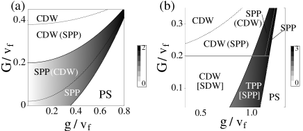
Figure 3: Phase diagrams for a mixture of bosonic and $S=1/2$ fermionic atoms. Shading in the paired regions describes the strength of bosonic screening clouds around fermionic polarons. In both figures $v_{b}/v_{f}=5$ and $K_{b}=10$. In (a) $U_{\uparrow\downarrow}/v_{f}=-0.8\pi$ and in (b) $U_{\uparrow\downarrow}/v_{f}=0.8\pi$. At the top of (b) and everywhere in (a) we have $g_{1\perp}<0$ ($K_{\sigma}<1$), and $g_{1\perp}<0$ ($K_{\sigma}>1$) at the bottom of (b). For larger $G$ and $U_{\uparrow\downarrow}$ one can also have a Wigner crystal phase (not shown here). Note that parentheses ($\dots$) indicate subdominant phases, while square brackets [$\dots$] indicate degenerate phases.

In summary, we used the bosonization method to investigate 1D mixtures of bosonic and fermionic atoms involving spinless and $S=1/2$ fermions. Interactions between atoms can lead to such interesting phenomena as spin and charge density waves, singlet and triplet pairing of atoms. This phase diagram can be understood in terms of polarons, in that it corresponds to a Luttinger liquid of polarons. We also discussed laser stirring experiments as a technique for probing quantum phase transitions between paired and insulating phases of polarons, and considered the finite temperature and size of a real system.

We thank B.I. Halperin for useful discussions. This work was supported by the NSF (grants DMR-01328074, PHY-0134776), the Sloan and the Packard Foundations, and by Harvard-MIT CUA. W.H. was supported by the German Science Foundation (DFG) and by the NSF (grant DMR-02-33773).

References

- (1) G. Modugno, et al., Science 297, 2240 (2002); F. Ferlaino et al., cond-mat/0312255; A. Simoni et al., cond-mat/0301159; B. Laburthe et al., cond-mat/0312003; T. Stöferle et al., cond-mat/0312440.
- (2) Z. Hadzibabic et al., Phys. Rev. Lett. 88, 160401 (2002); G. Roati, et al., Phys. Rev. Lett. 89, 150403 (2002); F. Schreck, et al., Phys. Rev. Lett. 87, 080403 (2001); A.G. Truscott, Science 291, 2570 (2001).
- (3) F. Matera, Phys. Rev A 68, 043624 (2003); D.V. Efremov and L. Viverit, Phys. Rev. B 65, 134519 (2002); L. Viverit, Phys. Rev. A 66, 023605 (2002).
- (4) M.Y. Kagan et. al., cond-mat/0209481; M. Lewenstein et. al., cond-mat/0306180; H. Fehrmann et. al., cond-mat/0307635.
- (5) R. Roth and K. Burnett, cond-mat/0310114
- (6) H.P. Büchler and G. Blatter, cond-mat/0304534; T. Miyakawa et al., cond-mat/0401107
- (7) A. Y. Kitaev, cond-mat/0010440
- (8) F. D. M. Haldane, Phys. Rev. Lett. 47, 1840 (1981).
- (9) M.A. Cazalilla, cond-mat/0307033.
- (10) A. Görlitz, et al. Phys. Rev. Lett. 87, 130402 (2001).
- (11) J. Solyom, Adv. Phys. 28, 201 (1979); J. Voit, Rep. Prog. Phys., 58, 977 (1995).
- (12) In this paper, we use to denote the optical lattice potential experienced by fermionic/bosonic atoms in the longitudinal (perpendicular) directions. Independent tuning of the optical lattices for two species of atoms can be achieved even with a single pair of lasers providing the standing beam. For example, the lattice strengths for bosons and fermions in longitudinal direction is given by and , where is the detuning of the bosonic state, is the energy difference between the bosonic and the fermionic state, and are the Rabi frequencies, which are propotional to the laser intensity. By controlling and the laser intensity, and can be varied independently over a wide range.
- (13) M. A. Cazalilla and A. F. Ho, Phys. Rev. Lett. 91, 150403 (2003).
- (14) A.P. Albus, et al., cond-mat/0211060; M.J. Bijlsma, et al., Phys. Rev. A 61, 053601 (2000).
- (15) D. Jaksch et. al., Phys.Rev.Lett. 81, 3108 (1998).
- (16) M. Kramer, et. al., Phys. Rev. Lett. 88, 180404 (2002).
- (17) In the case of half-filling for fermions we find that Umklapp processes are irrelevant (in the renormalization group (RG) sense) outside of the phase separation region in terms of experimental parameters. Hence, we do not expect a true long range charge order in the system.
- (18) J. Voit and Schulz, Phys. Reb. B 36, 968 (1987); ibid 37, 10068 (1988).
- (19) S. Engelsberg and B.B. Varga , Phys. Rev. 136, A1582 (1964).
- (20) We defined , , , , , and . is given by . Details of the calculations will appear elsewhere.
- (21) A.S. Alexandrov and S.N. Mott, Polarons and Bipolarons (World Scientific, Singapore, 1995).
- (22) C. Raman, et. al., Phys. Rev. Lett. 83, 2502 (1999); R. Onofrio, et. al., Phys. Rev. Lett. 85, 2228 (1999).
- (23) C. Kane and M.P.A. Fisher, Phys. Rev. Lett. 68, 1220 (1992).