Theory confronts experiment in the Casimir force measurements: quantification of errors and precision

Abstract

We compare theory and experiment in the Casimir force measurement between gold surfaces performed with the atomic force microscope. Both random and systematic experimental errors are found leading to a total absolute error equal to 8.5 pN at 95% confidence. In terms of the relative errors, experimental precision of 1.75% is obtained at the shortest separation of 62 nm at 95% confidence level (at 60% confidence the experimental precision of 1% is confirmed at the shortest separation). An independent determination of the accuracy of the theoretical calculations of the Casimir force and its application to the experimental configuration is carefully made. Special attention is paid to the sample-dependent variations of the optical tabulated data due to the presence of grains, contribution of surface plasmons, and errors introduced by the use of the proximity force theorem. Nonmultiplicative and diffraction-type contributions to the surface roughness corrections are examined. The electric forces due to patch potentials resulting from the polycrystalline nature of the gold films are estimated. The finite size and thermal effects are found to be negligible. The theoretical accuracy of about 1.69% and 1.1% are found at a separation 62 nm and 200 nm, respectively. Within the limits of experimental and theoretical errors very good agreement between experiment and theory is confirmed characterized by the root mean square deviation of about 3.5 pN within all measurement range. The conclusion is made that the Casimir force is stable relative to variations of the sample-dependent optical and electric properties, which opens new opportunities to use the Casimir effect for diagnostic purposes.

I Introduction

In the last few years the Casimir effect 1 , which is a rare macroscopic manifestation of the boundary dependence of the quantum vacuum, has attracted much experimental and theoretical attention (see monographs 2 ; 3 ; 4 and reviews 5 ; 6 ). The spectrum of the electromagnetic zero-point oscillations depends on the presence of material bodies. In particular, the tangential component of the electric field vanishes on the surfaces of two parallel plates made of ideal metal (it is small if real metals are used). This leads to changes in the zero-point oscillation spectrum compared to the case of free unbounded space and results in the attractive Casimir force acting normal to the surfaces of the plates.

The Casimir effect finds many applications in quantum field theory, condensed matter physics, elementary particle physics, gravitation and cosmology 2 ; 3 ; 4 ; 5 ; 6 . Recently many measurements of the Casimir force have been performed 7 ; 8 ; 9 ; 10 ; 11 ; 12 ; 13 ; 14 ; 15 ; 16 . Their results have already been applied in nanotechnology for the actuation of the novel microelectromechanical devices, based entirely on the modification of the properties of quantum vacuum 17 , and for constraining predictions of extra-dimensional physics with low compactification scales 14 ; 16 ; 18 ; 19 ; 20 ; 21 ; 22 .

Most theoretical papers on the Casimir effect deal with idealized boundary conditions and perfectly shaped test bodies. Over the last 4 decades only a few have considered the corrections to the Casimir force such as due to the finite conductivity of the boundary metal 23 ; 24 ; 25 , distortions of the surface shape 26 ; 27 and nonzero temperature 28 ; 29 . Comparison of the theory with the results of modern Casimir force measurements demands careful treatment of all these corrections. Both the individual corrections and their combined effect has to be evaluated (see Ref. 6 for review).

The quantification of errors and precision in the measurements and theoretical computations of the Casimir force is crucial for using the Casimir effect as a new test for extra-dimensional physics and other extensions to the Standard Model. Nevertheless, there is no general agreement on the achieved levels of experimental precision and the extent of agreement between theory and experiment. In the literature a variety of measures to characterize the experimental precision is used and the extent of agreement between measurements and theory ranges from 1% 8 ; 10 ; 11 ; 16 to 15% 13 depending on the measurement scheme and configuration. Very often, the confidence levels and numerous background effects which may contribute to the theoretical results are not considered.

In the present paper we perform a reanalysis of the experimental data on the Casimir force measurements between Au surfaces 11 and make a comparison with theory. In doing so we carefully calculate the original experimental precision without relation to the theory, including the random absolute error at a 95% confidence level, and the absolute systematic error. The total absolute error of these Casimir force measurements in the experiment of Ref. 11 is found to be equal to $\Delta^{tot}\approx 8.6\,$pN at 95% confidence. This corresponds to approximately 1.75% precision at the closest separation $a\approx 62\,$nm (the 1% precision at the closest separation indicated in Ref 11 is obtained at 60% confidence). As a second step, the accuracy of the theoretical computations of the Casimir force for the experimental configuration 11 is determined. Special attention is paid to the possible sample-dependent variations of the optical tabulated data due to the presence of grains, contribution of the surface plasmons, and errors introduced by the use of the proximity force theorem. The influence of the surface roughness is carefully investigated including the nonmultiplicative contributions and recently discussed diffraction-type effects 30 ; 31 . The contribution of electric forces due to patch potentials resulting from the polycrystalline nature of the Au film is calculated for the experimental configuration 11 at different separations. The finite size and thermal effects are also considered and found negligible in the experimental configuration of Ref. 11 . The conclusion reached is that at the present state of our knowledge the accuracies of theoretical computations in application to the experimental configuration of Ref. 11 are achievable on the level of 1.69% at a separation $z=62\,$nm and 1.1% at a separation $z=200\,$nm.

The paper is organized as follows. In Sec. II the experimental precision of the Casimir force measurements at different confidence levels is determined. Sec. III is devoted to the computations of the Casimir force with account of finite conductivity and grain structure of the metal layers. The role of roughness including the nonmultiplicative and diffraction-type effects is studied in Sec. IV. In Sec. V both traditional and alternative thermal corrections are discussed. Also the possible role of the electric forces due to the patch potentials and finite size effects are estimated. Sec. VI contains the final numbers on theoretical accuracy and the comparison of theory with experiment in the Casimir force measurement between two gold surfaces by means of an atomic force microscope 11 . In Sec. VII the final conclusions and some discussion are provided.

II Experimental precision in the Casimir force measurements between two gold surfaces

In Ref. 11 precision measurements of the Casimir force between gold coated bodies, a plane plate and a sphere, were performed using an atomic force microscope. The Casimir force was measured by averaging 30 scans over a surface separation region between 62–350 nm with 2583 points each (see Ref. 11 for all the details of the measurement procedure). In the analysis below we neglect data from 3 scans due to excessive noise and use the data from the rest $n=27$ scans to find the quantitative characteristics of the experimental precision in the Casimir force measurements at different confidence levels.

We start with the random error and calculate the mean values of the measured force at different separations $z_{i}$ within the region from 62 nm to 350 nm

$$\bar{F}^{exp}(z_{i})=\frac{1}{n}\sum\limits_{k=1}^{n}F_{k}^{exp}(z_{i}).$$ (1)

An estimate for the variance of this mean is determined by 32

$$s_{\bar{F}}^{2}(z_{i})=\frac{1}{n(n-1)}\sum\limits_{k=1}^{n}\left[F_{k}^{exp}(z_{i})-\bar{F}^{exp}(z_{i})\right]^{2}.$$ (2)

Calculations using the measurement data $\{F_{k}^{exp}(z_{i})\}$ show that $s_{\bar{F}}(z_{i})$ do not depend sensitively on $z_{i}$. The largest value $s_{\bar{F}}=2.8\,$pN is taken below as an estimate for the variance of the mean force within the whole measurement range.

According to Student’s test for the truth of a hypothesis 32 , if the inequality

$$\frac{|\bar{F}^{exp}(z)-F(z)|}{s_{\bar{F}}}>t_{\alpha}^{\prime}\equiv t_{1-\frac{1}{2}\alpha}$$ (3)

is fulfilled, the hypothesis that $F(z)$ is the true value of the Casimir force at a separation $z$ must be rejected at a given confidence level $\alpha$ (this is a two-tailed test as the deviations $F(z)$ from $\bar{F}^{exp}(z)$ in two directions are possible). Equivalently, if the inequality

$$\frac{|\bar{F}^{exp}(z)-F(z)|}{s_{\bar{F}}}\leq t_{1-\frac{1}{2}\alpha}$$ (4)

is fulfilled, the hypothesis that $F(z)$ is the true value of the Casimir force should be accepted at a confidence level $\beta=1-\alpha$.

Usually in the tables for Student’s $t$-distribution (see, e.g., Refs. 32 ; 33 ) the values of $t_{p}\equiv t_{p}(f)$ are presented, where $p=1-\alpha/2=(1+\beta)/2$, $f=n-1$ is the number of degrees of freedom, and $n$ is the number of measurements ($n=27$ in our case). Choosing $\beta=0.95$ (hypothesis is true at 95% confidence) we obtain $p=0.975$ and find from tables $t_{p}(f)=2.056$ 33 . Then from Eq. (4) it follows

$$|{\bar{F}}^{exp}(z)-F(z)|\leq\Delta^{rand}F^{exp}\equiv s_{\bar{F}}t_{p}(f)\approx 5.8\,\mbox{pN},$$ (5)

where $\Delta^{rand}F^{exp}$ is the random absolute error of the Casimir force measurements. If we consider $\beta=0.6$ (hypothesis is true at 60% confidence), then $p=0.8$ and $t_{p}(f)=0.856$. In this case the random absolute error of the Casimir force measurements is $\Delta^{rand}F^{exp}=2.8\times 0.856\,$pN$\approx 2.4\,$pN. Note that if one would like to have $t_{p}(f)=1$ or $t_{p}(f)=2$ (i.e. deviations of the true force value on either side of the mean not greater than one or two $s_{\bar{F}}$), the confidence levels of $\beta=0.66$ or $\beta=0.94$, respectively, should be chosen for the number of measurements $n=27$.

Now let us consider the systematic error. The main contributions to the systematic error in the experiment of Ref. 11 are given by the error in force calibration $\Delta_{1}^{syst}F^{exp}\approx 1.7\,$pN, by the noise when the calibration voltage is applied to the cantilever $\Delta_{2}^{syst}F^{exp}\approx 0.55\,$pN, by the instrumental sensitivity $\Delta_{3}^{syst}F^{exp}\approx 0.31\,$pN, and by the restrictions on computer resolution of data $\Delta_{4}^{syst}F^{exp}\approx 0.12\,$pN. The maximal value of the systematic error is given by

$$\Delta^{syst}F^{exp}=\sum\limits_{i=1}^{4}\Delta_{i}^{syst}F^{exp}\approx 2.7\,\mbox{pN}.$$ (6)

Finally, the maximum total absolute error of the Casimir force measurements in the experiment of Ref. 11 is equal to

$$\Delta F^{exp}=\Delta^{rand}F^{exp}+\Delta^{syst}F^{exp}\approx 8.5\,\mbox{pN}$$ (7)

at 95% confidence (to be conservative, the errors are added linearly rather than quadratically). At 60% confidence the total absolute error of the Casimir force measurements is $\Delta F^{exp}\approx 5.1\,$pN. These absolute errors with their confidence levels are valid within the whole measurement range from 62 nm to 350 nm. From Eq. (5) it follows that the true value of the Casimir force belongs to the confidence interval

$${\bar{F}}^{exp}(z)-\Delta F^{exp}\leq F(z)\leq{\bar{F}}^{exp}(z)+\Delta F^{exp}$$ (8)

with a chosen confidence probability.

Another important characteristic of the experimental precision is the relative error of the Casimir force measurements $\delta F^{exp}(z)=\Delta F^{exp}/{\bar{F}}^{exp}(z)$ which is evidently separation-dependent. At the shortest separation $z=62\,$nm the value of the mean force is ${\bar{F}}^{exp}=485.8\,$pN which leads to a relative error of $\delta F^{exp}(z)\approx 1.75$% computed at 95% confidence. If we restrict ourselves with a 60% confidence, the relative error of the Casimir force measurements at the shortest separation $\delta F^{exp}(z)=5.1/485.8\approx 1$% is obtained as was indicated in Ref. 11 without the detailed analysis of the confidence levels. If we choose 95% confidence, the relative errors of the Casimir force measurements at separations 70 nm, 100 nm, and 200 nm are, respectively, 2.46%, 5.9%, and 37.3%. At 60% confidence the relative errors of the Casimir force measurements at the same separations are 1.47%, 3.5%, and 22.4%, respectively.

III Calculation of the Casimir force including the finite conductivity and grain structure of gold layers

For the configuration of a large sphere of a radius $R$ above a plate the Casimir force can be obtained by means of the Lifshitz formula, derived originally for two parallel plates 34 , along with use of the proximity force theorem 35

$$F_{c}(z)=\frac{\hbar R}{2\pi}\int_{0}^{\infty}k_{\bot}dk_{\bot}\int_{0}^{\infty}d\xi\left\{\ln\left[1-r_{\|}^{2}(\xi,k_{\bot})e^{-2zq}\right]\right.$$

$$\phantom{aaaaaaaaaaa}\left.+\ln\left[1-r_{\bot}^{2}(\xi,k_{\bot})e^{-2zq}\right]\right\}.$$ (9)

Here the reflection coefficients for two independent polarizations are given by

$$r_{\|}^{2}(\xi,k_{\bot})=\left[\frac{\varepsilon(i\xi)q-k}{\varepsilon(i\xi)q+k}\right]^{2},\qquad r_{\bot}^{2}(\xi,k_{\bot})=\left(\frac{q-k}{q+k}\right)^{2},$$

$$q^{2}\equiv k_{\bot}^{2}+\frac{\xi^{2}}{c^{2}},\qquad k^{2}\equiv k_{\bot}^{2}+\varepsilon(i\xi)\frac{\xi^{2}}{c^{2}},$$ (10)

$\varepsilon(\omega)$ is the dielectric permittivity of the gold layers on the sphere and the plate, and $z$ is the closest separation distance between them. The thickness of gold coatings, used in Ref. 11 (86.6 nm), is much greater than the skin depth of the electromagnetic oscillations for all frequencies which make a significant contribution to the computation of the Casimir force. This allows one to use the properties of the bulk gold in all computations of the Casimir force.

The accuracy of Eq. (9) is restricted by the accuracy of the proximity force theorem, which is, however, very high for the experimental parameters of Ref. 11 . The error, introduced by the proximity force theorem, is less than $z/R$ 36 ; 37 . Taking into account the large value of sphere radius $R=95.65\,\mu$m, used in Ref. 11 , the upper limit of this error is 0.06% at the shortest separation $z=62\,$nm and 0.2% at separation $z=200\,$nm (note that in Ref. 36 the Casimir force for the configuration of a sphere above a plate was precisely computed on the basis of the first physical principles which makes it quite reliable as a test of the proximity force theorem).

In Refs. 38 ; 39 the computations of the Casimir force were performed using Eqs. (9), (10) and optical tabulated data for gold 40 (note that the transition coefficient from energies to frequencies is given by 1 eV$=1.52\times 10^{15}\,$rad/s). The imaginary part of the dielectric permittivity, obtained using the complex refractive index from the Tables 40 , was used to compute the dielectric permittivity along the imaginary frequency axis by means of the dispersion relation. At $\omega<1.9\times 10^{14}\,$rad/s, where the tabulated data are not immediately avaliable, they were usually obtained (see, e.g., 38 ; 39 ) by the extension from the region of higher frequencies by means of the Drude dielectric function

$$\varepsilon(\omega)=1-\frac{\omega_{p}^{2}}{\omega(\omega+i\gamma)}\,,$$ (11)

where the plasma frequency for Au is $\omega_{p}=1.37\times 10^{16}\,$rad/s, and $\gamma=5.32\times 10^{13}\,$rad/s is the relaxation parameter describing the non-elastic electron-phonon interaction (note that in the frequency region under consideration $\gamma\ll\omega$). This procedure was used to calculate the Casimir force including the effect of finite conductivity corrections of gold (see a few examples of the calculations in Sec. IV, Table II and comparison between experiment and theory in Sec. VI). Later in this section we discuss the influence of possible sample to sample variations of the optical tabulated data on the values of the Casimir force and the applicability region of Eqs. (9), (10) involving the dielectric permittivity depending only on frequency.

First, we would like to note that in the separation region $200\,\mbox{nm}<z<350\,$nm the computational results obtained by Eq. (9) combined with the optical tabulated data, are almost exactly those obtained by the substitution into Eq. (9) of the plasma dielectric function for the metal

$$\varepsilon(\omega)=1-\frac{\omega_{p}^{2}}{\omega^{2}}\,.$$ (12)

In fact, both computations lead to results differing by less than 0.5% within the mentioned separation region. What this means is that the real part of $\varepsilon$ depending on only $\omega_{p}$ determines the total value of the Casimir force in this region. The value of $\omega_{p}=2\sqrt{\pi N}e/\sqrt{m^{\ast}}$, where $N$ is the density of conduction electrons, $m^{\ast}$ is their effective mass, is determined by the preperties of the elementary cell. It cannot be influenced by properties of sample such as the crystallite grain size or the presence of a small concentration of impurities. This is the reason why the sample to sample variations of the optical tabulated data cannot influence the value of the Casimir force (9) at separations $z\geq 200\,$nm.

In the separation region $62\,\mbox{nm}<z<200\,$nm there are significant deviations depending on whether the Casimir force (9) is calculated using the optical tabulated data or by use of the plasma dielectric function (12). In fact, in this separation region the small imaginary part of $\varepsilon$ is influential and should be taken into account. There is enough tabulated data in the optical Tables to compute the Casimir force, so that it is not necessary to use any extension of data. Note that the characteristic frequency corresponding to the largest separation $z=200\,$nm is $\omega_{c}=c/(2z)=7.5\times 10^{14}\,$rad/s (i.e. tabulated data for frequencies several times smaller are available). At the same time, the characteristic frequency corresponding to the shortest separation is $\omega_{c}=2.42\times 10^{15}\,\mbox{rad/s}\ll\omega_{p}$, so that the region under consideration belongs to that of infrared optics 41 . Within the region (62–200)nm one may expect some small dependence of the optical tabulated data on the size of the grain, presence of impurities etc. If this is indeed the case, the use of the tabulated data, which are not relevant to the particular samples used in experiment, might lead to the errors in computation of the Casimir force (9).

To investigate this possibility, we consider the pure imaginary part of the dielectric permittivity in the region of the infrared optics given by 42

$$\mbox{Im}\varepsilon=\frac{\omega_{p}^{2}\nu}{\omega^{3}},$$ (13)

where $\nu$ is the relaxation parameter at high frequencies in the region of infrared optics (note that it does not coincide with the relaxation parameter $\gamma$ of the Drude model (11) which describes the volume relaxation in the region of the normal skin effect). The value of $\nu$ is determined by the processes of elastic scattering of the electrons on impurities, on the boundary surfaces of the metal and of the individual grains, and on other electrons 42 ; 43 . The scattering of electrons on phonons also contributes to the value of $\nu$. However, the frequency of the electromagnetic field is so high that $\hbar\omega\gg k_{B}T_{D}$, where $T_{D}$ is the Debye temperature, so the frequency of the electron-phonon collisions is the same as it is at $T=T_{D}$ 42 . It is important to note that of all the above processes, only the contribution of the electron-electron collisions to $\nu$ is frequency-dependent (and increases as $\omega^{2}$).

The main sample to sample dependence of the parameter $\nu$ is determined by the sizes of grains and the density of impurities. To calculate this dependence we use the following formula for the relaxation parameter in the region of infrared optics 42 ; 44

$$\nu=\omega_{p}\left(c_{1}+c_{2}\frac{\omega^{2}}{\omega_{p}^{2}}\right).$$ (14)

This formula leads to an approximate representation of the dielectric permittivity of Au along the imaginary frequency axis given by

$$\varepsilon(i\xi)=1+\frac{\omega_{p}^{2}}{\xi^{2}}-\frac{\omega_{p}^{3}}{\xi^{3}}\left(c_{1}-c_{2}\frac{\xi^{2}}{\omega_{p}^{2}}\right),$$ (15)

where $c_{1}=0.0039$, $c_{2}=1.5$. It is easily seen, that the substitution of Eq. (15) into Eq. (9) leads approximately to the same result as the use of the optical tabulated data. The errors due to use of Eq. (15) in Eq. (9) instead of the optical tabulated data at separations 62 nm, 70 nm, 100 nm, and 150 nm, are 0.45%, 0.23%, 0.09%, and 0.04%, respectively.

Eq. (15) gives the possibility to estimate the influence of the sizes of grains in the polycrystalline metal film in the experiment of Ref. 11 on the value of the Casimir force (9). For this purpose, the experimental data of Ref. 45 are used where the reflectance $R$ of Au films is measured as a function of the characteristic sizes of the grains.

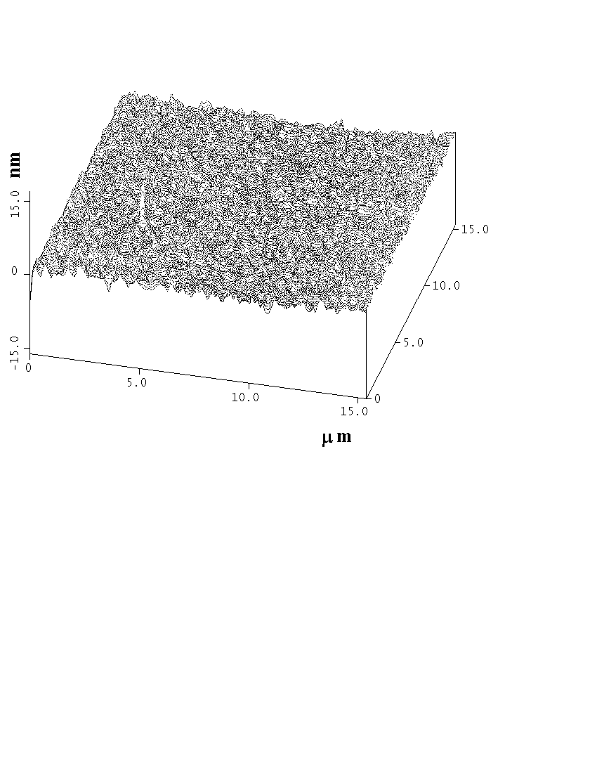
Figure 1: $15\times 15\,\mu\mbox{m}^{2}$ atomic force microscope image of the Au coating on the plate. The topography of the coating on the sphere is similar.

The analysis of the atomic force microscopy images (like the one in Fig. 1 but on $1\times 1\,\mu\mbox{m}^{2}$ area) shows that the mean size of grains in Ref. 11 is about 90 nm (the sizes of the typical grains are 77 nm, 103 nm, 94 nm, 68 nm, 88 nm, 121 nm etc). According to Ref. 45 , the largest deviations of the reflectance from the one given by the tabulated data 40 , takes place at shorter wavelengths. The shortest separation of $z=62\,$nm in the experiment 11 corresponds to the characteristic wavelength $\lambda_{c}=2\pi c/\omega_{c}=4\pi z\approx 780\,$nm. For the films containing grains of 45 nm size (the largest ones studied in Ref. 45 ) the reflectance at $\lambda\sim(750-800)$nm is 0.8% less than the one calculated from the tabulated data (notice that for smaller grains the difference of the reflectance obtained from the tabulated data is greater). Taking into account that the reflectance in the region of the infrared optics is given by 46

$$R=1-4\mbox{Re}\frac{1}{\sqrt{\varepsilon}}=\frac{\nu}{\omega_{p}},$$ (16)

we find that the new value for the coefficient $c_{1}$ in Eqs. (14), (15) due to grains of 45 nm size is ${\tilde{c}}_{1}=0.0059$. Substituting the approximate Eq. (15) (with ${\tilde{c}}_{1}$ instead of $c_{1}$) into Eq. (9), one finds the values of the correction factor to the Casimir force ${\tilde{\eta}}_{c}^{A}=0.439$ at $z=62\,$nm and ${\tilde{\eta}}_{c}^{A}=0.465$ at $z=70\,$nm. Comparing this with the results of the same approximate computations using $c_{1}$ ($\eta_{c}^{A}=0.441$, respectively, $\eta_{c}^{A}=0.467$), one can conclude that the grains of 45 nm size lead to less than 0.5% decrease of the Casimir force magnitude. Note that this is in fact the upper bound for the influence of crystallite grain size on the Casimir force in the experiment of Ref. 11 , as the actual sizes of grains in 11 were two times greater than 45 nm.

The above calculations of the Casimir force including the effect of the real properties of Au films were performed on the basis of the Lifshitz formula (9), which does not take into account the effects of spatial nonlocality (wavevector dependence of the dielectric permittivity). These effects may influence the Casimir force value in the region of the anomalous skin effect which is important for large separations $z>2.36\,\mu$m 47 , a region not relevant to the experiment of Ref. 11 . Another separation region, where nonlocality may lead to important contributions to the van der Waals force, is $z<\lambda_{p}/(4\pi)\approx 10.9\,$nm ($\lambda_{p}$ is the plasma wavelength) which corresponds to $\omega_{c}>\omega_{p}$ 48 . Such high characteristic frequencies lead to the propagation of surface plasmons. The effect of the surface plasmons, however, does not contribute in the experiment of Ref. 11 as the largest characteristic frequency there, calculated at $z=62\,$nm, is 5.7 times less than $\omega_{p}$ [notice that the frequency region ($5\omega_{c},10\omega_{c}$) contributes only 0.19% of the Casimir force value at separation $z=62\,$nm]. The contribution of the surface plasmon for Au of about 2% at a separation $z=\lambda_{p}=137\,$nm, obtained in recent Ref. 49 , is explained by the use in 49 of the spatially nonlocal dielectric permittivity in the frequency region of infrared optics where it is in fact local 41 ; 42 ; 46 (we would like to point out that at the separation $z=\lambda_{p}$ the characteristic frequency of the Casimir effect is equal not to $\omega_{p}$, as one might expect, but $\omega_{p}/(4\pi)$]. As a result, the surface plasmons do not give any contribution to the Casimir force in the experimental configuration of Ref. 11 .

IV Surface roughness correction to the Casimir force and its calculation using different approaches

It is well known that surface roughness corrections may play an important role in Casimir force calculations at separations less than 1 $\mu$m 6 . At the shortest separations, the roughness correction contributes 20% of the measured force in experiments of Refs. 8 ; 15 ; 16 . In the experiment of Ref. 11 , however, the roughness amplitude was decreased and the roughness contribution was made less than 1% of the measured force even at shortest separations. To obtain this conclusion the simple stochastic model for the surface roughness and the multiplicative approach to take into account different corrections were used. Here we obtain more exact results for the contribution of surface roughness to the Casimir force taking into account both nonmultiplicative and correlation effects.

The topography of the Au coatings on the plate and sphere was investigated using an atomic force microscope. A typical 3-dimensional image resulting from the surface scan of $15\,\mu\mbox{m}\times 15\,\mu$m area is shown in Fig. 1. As seen in this figure, the roughness is mostly represented by the stochastically distributed distortions with the typical heights of about 2–4 nm, and rare pointlike peaks with the heights up to 16 nm. In Table I the fractions $v_{i}$ of the surface area, shown in Fig. 1, with heights $h_{i}$ are presented ($i=1,2,\ldots,17$). These data allow one to determine the zero roughness level $H_{0}$ relative to which the mean value of the function, describing roughness, is zero (note that separations between different bodies in the Casimir force measurements are usually measured between the zero roughness levels 6 ):

$$\sum\limits_{i=1}^{17}\left(H_{0}-h_{i}\right)v_{i}=0.$$ (17)

Solving Eq. (17), one obtains $H_{0}\approx 2.734\,$nm. If the roughness is described by the regular (nonstochastic) functions $Af(x,y)$, where $|f(x,y)|\leq 1$, for the roughness amplitude it follows $A=h_{i}^{max}-H_{0}=13.266\,$nm.

In the framework of the additive approach the values of the Casimir force including the effect of finite conductivity $F_{c}(z)$, obtained in Sec. III, Eq. (9), can be used to calculate the effect of roughness. For this purpose, the values of $F_{c}$ should be geometrically averaged over all different possible separations between the rough surfaces weighted with the probability of each separation 6 ; 8 ; 16

$$F_{c,r}(z)=\sum\limits_{i,j=1}^{17}v_{i}v_{j}F_{c}(z+2H_{0}-h_{i}-h_{j}).$$ (18)

Note that Eq. (18) is not reduced to a simple multiplication of the correction factors due to finite conductivity and surface roughness but takes into account their combined (nonmultiplicative) effect.

An alternative method of calculating the corrections due to the stochastic surface roughness was used in Ref. 11 . According to the results of Ref. 50 , the Casimir force between a plate and a sphere made of ideal metal and covered by a stochastic roughness with an amplitude $A_{st}$ is given by

$$F_{r}(z)=F_{0}(z)\left[1+6\left(\frac{A_{st}}{z}\right)^{2}+45\left(\frac{A_{st}}{z}\right)^{4}\right],$$ (19)

where $F_{0}(z)=-\pi^{3}\hbar cR/(360z^{3})$ is the Casimir force between perfectly shaped plate and sphere of radius $R$. Then the Casimir force including both the finite conductivity of the boundary metal and surface roughness can be calculated as

$$F_{c,r}^{m}(z)=F_{c}(z)\left[1+6\left(\frac{A_{st}}{z}\right)^{2}+45\left(\frac{A_{st}}{z}\right)^{4}\right],$$ (20)

i.e. by means of the multiplicative procedure.

The variance of the random process describing the stochastic roughness is found by the formula

$$\delta_{st}^{2}=\sum\limits_{i=1}^{17}\left(H_{0}-h_{i}\right)^{2}v_{i}.$$ (21)

Using the data from Table I, one obtains the values for variance $\delta_{st}\approx 0.837\,$nm and for the amplitude of a random process $A_{st}=\sqrt{2}\delta_{st}\approx 1.18\,$nm. This value is slightly larger than the one obtained in Ref. 11 on the basis of less complete data on roughness topography.

Now we are in a position to compare the contribution of the surface roughness computed by Eq. (18), taking into account the combined effect of the roughness and finite conductivity, and by the multiplicative procedure of Eq. (20). In Table II the results for the correction factors $\eta_{c}=F_{c}/F_{0}$, $\eta_{r}=F_{r}/F_{0}$, $\eta_{c,r}=F_{c,r}/F_{0}$, and $\eta_{c,r}^{m}=\eta_{c}\eta_{r}$ are presented at the shortest separations $z=62\,$nm, 70 nm, 80 nm, and 90 nm, where the roughness corrections play some role. As is seen from Table II, both approaches lead to practically coincident results for the roughness correction factors due to the combined effect of finite conductivity and surface roughness. This means that for such small roughness as in Ref. 11 the multiplicative procedure is quite satisfactory (for larger roughness amplitudes, however, the nonmultiplicative contributions may be essential 8 ; 16 ). Note also that for $A_{st}\approx 1.18\,$nm the fourth order term in Eq. (20) practically does not contribute even at shortest separations and can be neglected as was done in Ref. 11 .

Both Eqs. (18) and (20) used above are based on the approximation of additive summation and do not take into account the diffraction-type effects which arise in the case of roughness described by the periodic functions with small periods $\lambda<z$ 30 or by the stochastic functions with small correlation length 31 . To estimate the value of the correlation length in our case, we consider the set of cross sections of the roughness image shown in Fig. 1.

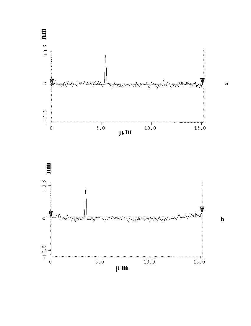
Figure 2: Typical cross sections of the atomic force microscope image of the Au coating on the plate with (a) constant $x$ and (b) constant $y$.

In Fig. 2 two typical cross sections are presented, one at fixed $x$ (a) and the other one at fixed $y$ (b). We have performed the Fourier analysis of the functions, as in Figs. 2,a,b, along the lines of Ref. 27 . It was found that the Fourier harmonics, giving the major contribution to the result, are characterized by significantly greater periods than the mean distance between the neighbouring peaks in Figs. 2,a,b which is equal, approximately, to 180 nm.

To obtain an estimate for the upper limit of the contribution of the diffraction-type effects in the above roughness analysis, we use the correlation length $l_{corr}=200\,$nm (slightly larger than the mean distance between peaks) and consider the periodic function with this period (clearly, the diffraction-type effects are greater for a periodic function with a period $l_{corr}$ than for the random function with a correlation length $l_{corr}$). With this the diffraction-type effects can be computed in the framework of the functional approach developed in Ref. 30 . At a shortest separation $z=62\,$nm one obtains $z/l_{corr}\approx 0.31$. Then for the coefficient $c_{corr}$ in the expression

$$\eta_{r}^{corr}=1+6c_{corr}\left(\frac{A_{st}}{z}\right)^{2},$$ (22)

taking the diffraction-type effects into account, from Fig. 2 of Ref. 30 it follows $c_{corr}\approx 1.1$. As a result, using the upper limit for the contribution of the diffraction effects one obtains $\eta_{r}^{corr}\approx 1.0024$, i.e. only 0.02% difference with the value of $\eta_{r}$ in Table II obtained by neglecting the diffraction effects. At larger separations the diffraction effects lead to larger contribution to the roughness corrections. For example, at a separation $z=90\,$nm we have $z/l_{corr}\approx 0.45$, $c_{corr}\approx 1.28$, and $\eta_{r}^{corr}\approx 1.0013$, i.e. 0.03% difference with the result of Table II. At larger separations, however, the roughness correction itself is even more negligible than at the shortest separations.

To conclude, the surface roughness contribution in the experiment of Ref. 11 does not exceed 0.24% of the Casimir force at the shortest separation $z=62\,$nm. The diffraction-type effects, which were not taken into account in Eqs. (18), (20), are shown to contribute less than one tenth of this result.

V Contributions of the thermal corrections, residual electric forces and finite sizes of the plate

Although the experiment of Ref. 11 was performed at room temperature $T=300\,$K, all the above computations were done at zero temperature. The thermal Casimir force $F_{c}(z,T)$ is given by Eq. (9) where integration in continuous $\xi$ is changed to a summation over the discrete Matsubara frequencies $\xi_{l}=2\pi k_{B}Tl/\hbar$ according to

$$\int_{0}^{\infty}d\xi\to\frac{2\pi k_{B}T}{\hbar}\sum\limits_{l=0}^{\infty}{\vphantom{\sum}}^{\prime},$$

leading to the Lifshitz formula for the thermal Casimir force. Here prime refers to the addition of a multiple 1/2 near the term with $l=0$. When $T\to 0$, $F_{c}(z,T)\to F_{c}(z,0)=F_{c}(z)$, where $F_{c}(z)$ is given by Eq. (9).

The magnitude of the relative thermal correction to the Casimir force can be computed by the formula

$$\delta_{T}F_{c}(z,T)=\frac{F_{c}(z,T)-F_{c}(z)}{F_{c}(z)}\equiv\frac{\Delta_{T}F_{c}(z,T)}{F_{c}(z)}.$$ (23)

Recently, there has been extensive discussion in literature on the correct calculation procedure for the thermal Casimir force $F_{c}(z,T)$ 47 . In Refs.  51 ; 52 the dielectric permittivity of the plasma model (12) was substituted into the Lifshitz formula for $F_{c}(z,T)$. This approach, which was later called “traditional” 15 , leads to the thermal corrections $\Delta_{T}^{tr}F_{c}$, $\delta_{T}^{tr}F_{c}$. It is consistent with thermodynamics and agrees with the limiting case of the ideal metal. In the region of infrared optics the same results were obtained in the framework of the impedance approach which does not consider the fluctuating electromagnetic field inside the metal and takes into account the realistic properties of the metal by means of the Leontovich boundary condition 47 ; 53 . Within the separation distances of Ref. 11 , the traditional thermal corrections are very small. As an example, at a separation $z=100\,$nm and $T=300\,$K one has $\delta_{T}^{tr}F_{c}\approx 0.007$%, and $\delta_{T}^{tr}F_{c}\approx 0.03$%, 0.1% at separations $z=200\,$nm, respectively, 300 nm 54 (to compare, in the case of ideal metals the same corrections, found in the framework of the thermal quantum field theory, are equal to 0.003%, 0.024%, and 0.08%, respectively, i.e. the results for real metals approach the results for ideal ones with the increase of separation 29 ; 54 ). Thus, the traditional thermal corrections are negligible in the measurement range of experiment 11 (the contribution of the relaxation processes to the magnitude of these corrections, which can be computed by taking into account the small real part of the surface impedance, is much less than the corrections).

Alternatively, in Refs. 55 ; 56 the dielectric permittivity of the Drude model (11) was used to calculate $F_{c}(z,T)$. In this approach, there is no continuous transition between the cases of real and ideal metal. At the high temperature limit, the Casimir force between real metals was found equal to one half of the result obtained for the ideal metal (independently of how high the conductivity of real metal is). The thermal corrections, computed in the framework of the alternative approach 55 ; 56 , are quite different from those obtained from the traditional approach. To find the magnitude of these corrections 54 , one should substitude into Eq. (23)

$$\Delta_{T}F_{c}(z,T)\equiv\Delta_{T}^{(1)}F_{c}(z,T)\approx\Delta_{T}^{tr}F_{c}(z,T)-\frac{k_{B}TR}{8a^{2}}\int_{0}^{\infty}ydy\ln\left[1-r_{\bot}^{2}(0,y)e^{-y}\right],$$ (24)

where $r_{\bot}^{2}(0,y)$ is obtained by the substitution of Eq. (12) into Eq. (10). After calculations, one obtains that the alternative relative thermal correction increases from $\delta_{T}^{(1)}F_{c}\approx 1.1$% and 1.3% at separations $z=62\,$nm, respectively, 70 nm to $\delta_{T}^{(1)}F_{c}\approx 8$% at a separation $z=350\,$nm.

Another alternative thermal correction suggested in literature 57 is also based on the substitution of the Drude dielectric function (11) into the Lifshitz formula for $F_{c}(z,T)$ but with a modified zero-frequency contribution for the perpendicular mode (in Ref. 57 this contribution is postulated to be of the same value as for an ideal metal). The alternative thermal correction of Ref. 57 is given by 54

$$\Delta_{T}F_{c}(z,T)\equiv\Delta_{T}^{(2)}F_{c}(z,T)\approx\Delta_{T}^{(1)}F_{c}(z,T)+\frac{k_{B}TR}{8a^{2}}\int_{0}^{\infty}ydy\ln\left(1-e^{-y}\right).$$ (25)

As a result, the relative alternative thermal correction of this kind takes values $\delta_{T}^{(2)}F_{c}\approx(2.1-2.2)$% at all separations from $z=62\,$nm to $z=350\,$nm, i.e. slightly larger than the experimental precision at the shortest separations.

As was shown in Ref. 58 , both alternative thermal corrections of Refs. 55 ; 56 and of Ref. 57 are not consistent with thermodynamics leading to the violation of the Nernst heat theorem. Recently they were found to be in disagreement with the precision measurement of the Casimir force using a microelectromechanical torsional oscillator 15 . In Sec. VI we will discuss the influence of the alternative thermal corrections on the comparison of theory and experiment in the Casimir force measurement of Ref. 11 .

In the rest of this section we discuss the probable contribution of the residual electric forces and the finite sizes of the plate on the Casimir force. As was noted in Ref. 11 , the electrostatic force due to the residual potential difference between the plate and the sphere has been lowered to negligible levels of $\ll 1$% of the Casimir force at the closest separations. In recent Ref. 59 it was argued, however, that the spatial variations of the surface potentials due to the grains of polycrystalline metal (the so called “patch potentials”) may mimic the Casimir force. Here we apply the general results of Ref. 59 to the experiment of Ref. 11 and demonstrate that the patch effect does not make significant contributions.

According to Ref. 59 , for the configuration of a sphere above a plate the electric force due to random variations in patch potentials is given by

$$F_{p}(z)=-\frac{4\pi\varepsilon_{0}\sigma_{v}^{2}R}{k_{\max}^{2}-k_{\min}^{2}}\int_{k_{\min}}^{k_{\max}}\frac{k^{2}e^{-kz}dk}{\sinh kz},$$ (26)

where $\sigma_{v}$ is the variance of the potential distribution, $k_{\max}$ ($k_{\min}$) are the magnitudes of the extremal wavevectors corresponding to minimal (maximal) sizes of grains, and $\varepsilon_{0}$ is the dielectric permittivity of free space. The work functions of gold are $V_{1}=5.47\,$eV, $V_{2}=5.37\,$eV, and $V_{3}=5.31\,$eV for different crystallographic surface orientations (100), (110), and (111), respectively. Assuming equal areas of these crystallographic planes one obtains

$$\sigma_{v}=\frac{1}{\sqrt{2}}\left[\sum\limits_{i=1}^{3}(V_{i}-\bar{V})^{2}\right]^{1/2}\approx 80.8\,\mbox{mV}.$$ (27)

Using the atomic force microscopy images discussed in Sec. III, the extremal sizes of grains in gold layers covering the test bodies were determined $\lambda_{\min}\approx 68\,$nm, and $\lambda_{\max}\approx 121\,$nm. This leads to $k_{\max}\approx 0.092\,\mbox{nm}^{-1}$ and $k_{\min}\approx 0.052\,\mbox{nm}^{-1}$. Note that these grain sizes are of the same order as the thickness of the film. The computations by Eq. (26) using the above data lead to the “patch effect” electric forces $F_{p}/R\approx-1.15\times 10^{-8}\,$N/m and $-1.25\times 10^{-10}\,$N/m at separations $z=62\,$nm and $z=100\,$nm, respectively. Comparing the obtained results with the values of the Casimir force at the same separations ($F_{c}/R\approx-5.06\times 10^{-6}\,$N/m, respectively, $-1.48\times 10^{-6}\,$N/m), we conclude that the electric force due to the patch potentials contributes only 0.23% and 0.008% of the Casimir force at separations $z=62\,$nm, respectively, $z=100\,$nm (at a separation $z=200\,$nm the patch effect contributes only $7\times 10^{-7}$% of the Casimir force. So a rapid decrease of the contribution of the electric force with an increase of a separation is explained by the exponential decrease of the integral in Eq. (26) if one substitutes the physical values of the integration limits based on the properties of gold films used in experiment of Ref. 11 .

A more important contribution of the patch electric forces may be expected in the scanning of a sharp tip of the atomic force microscope at a height of about 10–20 nm above a plate. In this case the electric forces are comparable with the van der Waals forces complicating the theoretical interpretation of force-distance relations 60 .

Let us finally estimate the theoretical error caused by finiteness of the plate used in the experiment of Ref. 11 . Eq. (9) was derived for the plate of infinite radius. In fact, the radius of the plate used in the experiment 11 is $L=5\times 10^{-3}\,$m. In this case, the Casimir force can be obtained by the formula 61

$$F_{c}^{fin}(z)=F_{c}(z)\beta(z)=\left[1-\frac{z^{3}}{R^{3}}\left(1-\frac{1}{\sqrt{1+L^{2}/R^{2}}}\right)^{-3}\right]F_{c}(z).$$ (28)

To calculate $\beta(z)$, we put $z=350\,$nm (to make this factor maximally distinct from unity) and obtain

$$\beta(z)\approx 1-8\frac{z^{3}R^{3}}{L^{6}}\approx 1-2.2\times 10^{-17},$$

i.e. the finiteness of the plate size is too small to give any meaningful contributions to the Casimir force.

VI Theoretical accuracy and comparison of theory and experiment

Now we are in a position to list all the sources of errors in the theoretical computation of the Casimir force $F_{c,r}$ given by Eq. (18), to find the final theoretical accuracy and to consider the comparison of theory and experiment.

The main error, which arises from Eqs. (9), (18) when one substitutes the experimental data, is due to the errors in determination of separation $z$ and sphere radius $R$. In terms of dimensionless variables, $F_{c,r}(z)$ is proportional to $R$ and inversely proportional to $z^{3}$ which results in

$$\delta^{(1)}F_{c,r}=\frac{\Delta F_{c,r}}{F_{c,r}}\approx\frac{\Delta R}{R}+3\frac{\Delta z}{z}.$$ (29)

In Ref. 11 the absolute separations were determined by means of the electric measurements which allowed the determination of the average separation distance on contact $z_{0}$ with the absolute error $\Delta^{el}z_{0}\approx 1\,$nm. Contrary to the opinion expressed in Ref. 62 , this error should not be transferred to all separations leading to rather large contribution to $\delta^{(1)}F_{c,r}$ of about $3\Delta^{el}z_{0}/z\approx 4.8$% at the shortest separations. Note that we are comparing not one experimental point with one theoretical value, but the experimental force-distance relation with the theoretical one computed on the basis of a fundamental theory. Thus, an additional fit should be made, with $z_{0}$ as a fitting parameter changing within the limits ($z_{0}-\Delta^{el}z_{0},z_{0}+\Delta^{el}z_{0}$) to achieve the smallest root mean square (r.m.s.) deviations between experiment and theory

$$\sigma_{M}=\left\{\frac{1}{M}\sum\limits_{i=1}^{M}\left[F_{c,r}(z_{i})-{\bar{F}}^{exp}(z_{i})\right]\right\}^{1/2},$$ (30)

where ${\bar{F}}^{exp}(z_{i})$ was defined in Eq. (1), $F_{c,r}(z_{i})$ were computed by Eq. (18), and $M$ is the number of experimental points under consideration. If, as usual, we consider two hypotheses as equivalent when they lead to the r.m.s. deviations differing for less than 10%, this results in decrease of the error in determination of absolute separations up to $\Delta z\approx 0.15\,$nm.

It is important to underline that the verification of the hypothesis is performed within different separation intervals (i.e. the total number $M=N=2583$ experimental points within the whole separation range from 62 nm to 350 nm, $M=1270$ points belonging to the interval 62–210 nm, and $M=600$ points at separations less than the plasma wavelength $\lambda_{p}=136\,$nm). The above value for $\Delta z$ is almost one and the same in all the separation intervals. The obtained values of the r.m.s. deviations between theory and experiment are $\sigma_{N}\approx 3.4\,$pN, $\sigma_{1270}\approx 3.2\,$pN, and $\sigma_{600}\approx 3.8\,$pN. These values are rather homogeneous demonstrating good agreement between theory and experiment independently of the chosen separation region.

The radius of the sphere was measured more precisely than in Ref. 11 with a result $2R=191.3\pm 0.3\,\mu$m. Using this together with $\Delta z=0.15\,$nm, one obtains from Eq. (29) at the shortest separations $\delta^{(1)}F_{c,r}\approx 0.88$%.

Now let us list the other contributions to the theoretical error of the Casimir force computations at the shortest separation $z=62\,$nm and indicate their magnitude. According to the results of Sec. III, the sample to sample variations of the optical tabulated data may lead to the decrease of the Casimir force magnitude for no more than $\delta^{(2)}F_{c,r}\approx 0.5$%. The use of the proximity force theorem at $z=62\,$nm leads to very small error of about $\delta^{(2)}F_{c,r}\approx 0.06$% (Sec. III). The corrections due to the surface roughness are already incorporated in the theoretical expression (18) but the diffraction-type effects may contribute up to $\delta^{(4)}F_{c,r}\approx 0.02$% (Sec. IV). The effect of electric forces due to the patch potentials contribute a maximum $\delta^{(5)}F_{c,r}\approx 0.23$% at the shortest separations, as was shown in Sec. V. The corrections due to the surface plasmons and finite size of the plate are negligible for the separation distances and experimental configuration used in Ref. 11 (see Secs. III and V).

Special attention should be paid to the thermal corrections to the Casimir force. According to the results of Sec. V, the contribution of the traditional thermal correction at the shortest separation is negligible. At larger separations it may be incorporated into the theoretical expression for the force. As to the alternative thermal corrections of Refs. 55 ; 56 ; 57 , which contribute of about (1–2)% of the Casimir force at the separation $z=62\,$nm, they have been already ruled out both experimentally and theoretically (see Sec. V). If we would include any of these corrections into the theoretical expression for the Casimir force, this results in the increase of the r.m.s. deviation between theory and experiment which cannot be compensated by shifts of the separation distance in the limit of error $\Delta^{el}z_{0}$. In view of the above, we exclude the contributions from these hypothetical corrections from our error analysis.

The upper limit for the total theoretical error at a separation $z=62\,$nm can be found by the summation of the above contributions

$$\delta F_{c,r}=\sum\limits_{i=1}^{5}\delta^{(i)}F_{c,r}\approx 1.69\mbox{\%},$$ (31)

which is a bit more accurate than the total experimental relative error at the shortest separation equal to 1.75% at 95% confidence (see Sec. II).

Note that with the increase of separation the experimental relative error quickly increases to 37.3% at a separation $z=200\,$nm. At the same time, the theoretical error is slowly decreasing with increasing separation. Thus, at $z=200\,$nm the above contributions to the theoretical error of the Casimir force computations take values $\delta^{(1)}F_{c,r}\approx 0.38$%, $\delta^{(2)}F_{c,r}\approx 0.5$%, $\delta^{(3)}F_{c,r}\approx 0.21$%, $\delta^{(4)}F_{c,r}\approx 0.026$%, $\delta^{(5)}F_{c,r}\approx 0.000$%. As a result, the total theoretical error at $z=200\,$nm is $\delta F_{c,r}\approx 1.1$%.

The obtained results demonstrate very good agreement between theory and experiment within the limits of both experimental and theoretical errors.

VII Conclusions and discussion

In this paper we have performed a detailed comparison of experiment and theory in the Casimir force measurement between the gold coated plate and sphere by means of an atomic force microscope 11 . The random error of the experimental values of the Casimir force was found to be $\Delta^{rand}F^{exp}\approx 5.8\,$pN at 95% confidence (at 60% confidence the value $\Delta^{rand}F^{exp}\approx 2.4\,$pN was obtained). Together with the systematic error $\Delta^{syst}F^{exp}\approx 2.7\,$pN, this leads to the total absolute error of the Casimir force measurements in Ref. 11 $\Delta{}F^{exp}\approx 8.5\,$pN at 95% confidence. In terms of the relative errors, the experimental precision at the shortest reported separation is equal to 1.75% (1%) at 95% (60%) confidence level.

In order to find the theoretical accuracy of the Casimir force calculations in the experimental configuration of Ref. 11 , many corrections to the ideal Casimir force were analysed. The correction due to the finite conductivity of gold was computed by the use of the optical tabulated data of the complex refractive index. The results were compared with those computed by the use of the plasma dielectric function and found to coincide for the surface separation range (200–350)nm. At shorter separations the use of the optical tabulated data more accurately represents the dielectric properties. A special model was presented, which allows to take into account the sample to sample variations of the optical tabulated data due to the sizes of grains and impurities. It was shown that the error introduced by the grains of 45 nm size (even smaller than those in the experiment of Ref.11 ) does not exceed 0.5% of the Casimir force. The influence of the surface plasmon in the separation region of the experiment 11 was found to be negligible.

The surface roughness of the test bodies, used to measure the Casimir force, was carefully investigated by means of the atomic force microscope with a sharp tipped cantilever instead of a large sphere. The obtained profiles of roughness topography allowed calculation of the roughness corrections to the Casimir force in the framework of both multiplicative and nonmultiplicative approaches. The minor differences in the size of the effect are found only at the shortest separation. The correlation length of the surface roughness on the test bodies was estimated and the diffraction-type effects were computed. At the shortest separation the roughness correction contributes 0.24% of the Casimir force with account of diffraction-type effects (and 0.22% with no account of diffraction).

The electric forces caused by the spatial variations of the surface potentials due to the size of grains were investigated for the experimental configuration of Ref. 11 . They were shown to contribute 0.23% of the Casimir force at the shortest separation, and this contribution quickly decreases with an increase of separation. Several other effects (such as thermal corrections, corrections due to the finiteness of the plate and due to the deviation from the proximity force theorem) were investigated and found to make only negligible contributions.

The final theoretical accuracy of the Casimir force calculations in the experimental configuration of Ref. 11 is 1.69% at the shortest separation $z=62\,$nm and 1.1% at a separation $z=200\,$nm. In the limits of both experimental and theoretical errors, very good agreement between theory and experiment was demonstrated characterized by the r.m.s. deviation of about 3.5 pN (less than 1% of the measured force at a shortest separation) which is almost independent of the separation region and the number of the experimental points. The above analysis does not support the conclusion of Ref. 62 that to achieve the experiments on the Casimir effect with 1% precision it is necessary to measure the separation on contact $z_{0}$ with atomic precision.

The obtained results demonstrate that in fact the Casimir force is more stable, than one might expect, to some delicate properties of the metallized test bodies like the variations of the optical data, patch potentials, correlation effects of roughness etc. These properties may change from sample to sample leaving the basic character, and even the values of the Casimir force within some definite separation region, almost unchanged. The stability of the Casimir force opens new opportunities to use the Casimir effect as a test for long-range hypothetical interactions and for the diagnostic purposes. For example, some kind of the inverse problem could be utilized, i.e. the measured force-distance relations be exploited to determine the fundamental characteristics of solids (such as the plasma frequency).

Table 1: Fractions $v_{i}$ of the surface area covered by roughness with heights $h_{i}$.

i	$h_{i}$ (nm)	$v_{i}$
1	0	$1.06\times 10^{-3}$
2	1	$5.086\times 10^{-2}$
3	2	$0.33511$
4	3	$0.45863$
5	4	$0.13695$
6	5	$1.586\times 10^{-2}$
7	6	$1.24\times 10^{-3}$
8	7	$1.6\times 10^{-4}$
9	8	$4\times 10^{-5}$
10	9	$2\times 10^{-5}$
11	10	$1\times 10^{-5}$
12	11	$1\times 10^{-5}$
13	12	$1\times 10^{-5}$
14	13	$1\times 10^{-5}$
15	14	$1\times 10^{-5}$
16	15	$1.2\times 10^{-5}$
17	16	$8\times 10^{-6}$

Table 2: Corrections factors to the ideal Casimir force at different separations due to finite conductivity ($\eta_{c}$), surface roughness ($\eta_{r}$) and both finite conductivity and surface roughness ($\eta_{c,r}$ and $\eta_{c,r}^{m}$ in the method of the geometrical averaging and in the multiplicative approach, respectively).

	$z=62\,$nm	$z=70\,$nm	$z=80\,$nm	$z=90\,$nm
$\eta_{c}$	0.4430	0.4681	0.4964	0.5218
$\eta_{r}$	1.0022	1.0017	1.0013	1.0010
$\eta_{c,r}$	0.4436	0.4687	0.4669	0.5223
$\eta_{c,r}^{m}$	0.4440	0.4689	0.4670	0.5223

References

- (1) H. B. G. Casimir, Proc. K. Ned. Akad. Wet. 51, 793 (1948).
- (2) P. W. Milonni, The Quantum Vacuum (Academic Press, San Diego, 1994).
- (3) V. M. Mostepanenko and N. N. Trunov, The Casimir Effect and its Applications (Clarendon Press, Oxford, 1997).
- (4) K. A. Milton, The Casimir Effect (World Scientific, Singapore, 2001).
- (5) M. Kardar and R. Golestanian, Rev. Mod. Phys. 71, 1233 (1999).
- (6) M. Bordag, U. Mohideen, and V. M. Mostepanenko, Phys. Rep. 353, 1 (2001).
- (7) S. K. Lamoreaux, Phys. Rev. Lett. 78, 5 (1997).
- (8) U. Mohideen and A. Roy, Phys. Rev. Lett. 81, 4549 (1998); G. L. Klimchitskaya, A. Roy, U. Mohideen, and V. M. Mostepanenko, Phys. Rev. A 60, 3487 (1999).
- (9) A. Roy and U. Mohideen, Phys. Rev. Lett. 82, 4380 (1999).
- (10) A. Roy, C.-Y. Lin, and U. Mohideen, Phys. Rev. D 60, 111101(R) (1999).
- (11) B. W. Harris, F. Chen, and U. Mohideen, Phys. Rev. A 62, 052109 (2000).
- (12) T. Ederth, Phys. Rev. A 62, 062104 (2000).
- (13) G. Bressi, G. Carugno, R. Onofrio, and G. Ruoso, Phys. Rev. Lett. 88, 041804 (2002).
- (14) F. Chen, U. Mohideen, G. L. Klimchitskaya, and V. M. Mostepanenko, Phys. Rev. Lett. 88, 101801 (2002); Phys. Rev. A 66, 032113 (2002).
- (15) R. S. Decca, D. López, E. Fischbach, and D. E. Krause, Phys. Rev. Lett. 91, 050402 (2003).
- (16) R. S. Decca, E. Fischbach, G. L. Klimchitskaya, D. E. Krause, D. López, and V. M. Mostepanenko, Phys. Rev. D 68, 116003 (2003).
- (17) H. B. Chan, V. A. Aksyuk, R. N. Kleiman, D. J. Bishop, and F. Capasso, Science, 291, 1941 (2001); Phys. Rev. Lett. 87, 211801 (2001).
- (18) M. Bordag, B. Geyer, G. L. Klimchitskaya, and V. M. Mostepanenko, Phys. Rev. D 58, 075003 (1998); 60, 055004 (1999); 62, 011701(R) (2000).
- (19) J. C. Long, H. W. Chan, and J. C. Price, Nucl. Phys. B 539, 23 (1999).
- (20) V. M. Mostepanenko and M. Novello, Phys. Rev. D 63, 115003 (2001).
- (21) E. Fischbach, D. E. Krause, V. M. Mostepanenko, and M. Novello, Phys. Rev. D 64, 075010 (2001).
- (22) G. L. Klimchitskaya and U. Mohideen, Int. J. Mod. Phys. A 17, 4143 (2002).
- (23) C. H. Hargreaves, Proc. Kon. Nederl. Acad. Wet. B 68, 231 (1965).
- (24) J. Schwinger, L. L. DeRaad, Jr., and K. A. Milton, Ann. Phys. (N.Y.) 115, 1 (1978).
- (25) V. M. Mostepanenko and N. N. Trunov, Yad. Fiz. 42, 1297 (1985) [Sov. J. Nucl. Phys. 42, 818 (1985)].
- (26) A. A. Maradudin and P. Mazur, Phys. Rev. B 22, 1677 (1980).
- (27) M. Bordag, G. L. Klimchitskaya, and V. M. Mostepanenko, Int. J. Mod. Phys. A 10, 2661 (1995).
- (28) J. Mehra, Physica 37, 145 (1967).
- (29) L. S. Brown and G. J. Maclay, Phys. Rev. 184, 1272 (1969).
- (30) T. Emig, A. Hanke, R. Golestanian, and M. Kardar, Phys. Rev. Lett. 87, 260402 (2001); Phys. Rev. A 67, 022114 (2003).
- (31) C. Genet, A. Lambrecht, P. Maia Neto, and S. Reynaud, Europhys. Lett. 62, 484 (2003).
- (32) S. Brandt, Statistical and Computational Methods in Data Analysis (North-Holland Publishing Company, Amsterdam, 1976).
- (33) CRC Handbook of Chemistry and Physics, eds. R. C. Weast and M. J. Astle, (CRC Press, Inc., Boca Raton, 1982).
- (34) I. E. Dzyaloshinskii, E. M. Lifshitz, and L. P. Pitaevskii, Usp. Fiz. Nauk 73, 381 (1961) [Sov. Phys. Usp. (USA) 4, 153 (1961)].
- (35) J. Blocki, J. Randrup, W. J. Swiatecki, and C. F. Tsang, Ann. Phys. (N.Y.) 105, 427 (1977).
- (36) P. Johansson and P. Apell, Phys. Rev. B 56, 4159 (1997).
- (37) M. Schaden and L. Spruch, Phys. Rev. A 58, 935 (1998).
- (38) A. Lambrecht and S. Reynaud, Eur. Phys. J. D 8, 309 (2000).
- (39) G. L. Klimchitskaya, U. Mohideen, and V. M. Mostepanenko, Phys. Rev. A 61, 062107 (2000).
- (40) Handbook of Optical Constants of Solids, ed. E. D. Palik (Academic, New York, 1985).
- (41) E. M. Lifshitz and L. P. Pitaevskii, Physical Kinetics (Pergamon Press, Oxford, 1981).
- (42) I. M. Lifshitz, M. Ya. Asbel’, and M. I. Kaganov, Electron Theory of Metals (Consultants Bureau, New York, 1973).
- (43) L. P. Pitaevskii, Zh. Eksp. Teor. Fiz. 34, 942 (1958) [Sov. Phys. JETP 34, 652 (1958)].
- (44) I. M. Kaganova and M. I. Kaganov, Phys. Rev. B 63, 054202 (2001).
- (45) J. Sotelo, J. Ederth, and G. Niklasson, Phys. Rev. B 67, 195106 (2003).
- (46) L. D. Landau, E. M. Lifshitz, and L. P. Pitaevskii, Electrodynamics of Continuous Media (Pergamon Press, Oxford, 1984).
- (47) B. Geyer, G. L. Klimchitskaya, and V. M. Mostepanenko, Phys. Rev. A 67, 062102 (2003).
- (48) J. Heinrichs, Phys. Rev. B. 11, 3625 (1975); 11, 3637 (1975); 12, 6006 (1975).
- (49) R. Esquivel, C. Villarreal, and W. L. Mochán, Phys. Rev. A, 68, 052103 (2003).
- (50) M. Bordag, G. L. Klimchitskaya, and V. M. Mostepanenko, Phys. Lett. A 200, 95 (1995).
- (51) C. Genet, A. Lambrecht, and S. Reynaud, Phys. Rev. A 62, 012110 (2000).
- (52) M. Bordag, B. Geyer, G. L. Klimchitskaya, and V. M. Mostepanenko, Phys. Rev. Lett. 85, 503 (2000); 87, 259102 (2001).
- (53) V. B. Bezerra, G. L. Klimchitskaya, and C. Romero, Phys. Rev. A 65, 012111 (2002).
- (54) G. L. Klimchitskaya and V. M. Mostepanenko, Phys. Rev. A 63, 062108 (2001).
- (55) M. Boström and B. E. Sernelius, Phys. Rev. Lett. 84, 4757 (2000).
- (56) J. S. Høye, I. Brevik, J. B. Aarseth, and K. A. Milton, Phys. Rev. E 67, 056116 (2003).
- (57) V. B. Svetovoy and M. V. Lokhanin, Phys. Lett. A 280, 177 (2001).
- (58) V. B. Bezerra, G. L. Klimchitskaya, and V. M. Mostepanenko, Phys. Rev. A 66, 062112 (2002).
- (59) C. C. Speake and C. Trenkel, Phys. Rev. Lett. 90, 160403 (2003).
- (60) N. A. Burnham, R. J. Colton, and H. M. Pollock, Phys. Rev. Lett. 69, 144 (1992).
- (61) V. B. Bezerra, G. L. Klimchitskaya, and C. Romero, Mod. Phys. Lett. A 12, 2623 (1997).
- (62) D. Iannuzzi, I. Gelfand, M. Lisanti, and F. Capasso, quant-ph/0312043.