Model for Entangled States with Spin-Spin Interaction

Abstract

A system consisting of two neutral spin 1/2 particles is analyzed for two magnetic field perturbations: 1) an inhomogeneous magnetic field over all space, and 2) external fields over a half space containing only one of the particles. The field is chosen to point from one particle to the other, which results in essentially a one-dimensional problem. A number of interesting features are revealed for the first case: the singlet, which has zero potential energy in the unperturbed case, remains unstable in the perturbing field. The spin zero component of the triplet evolves into a bound state with a double well potential, with the possibility of tunneling. Superposition states can be constructed which oscillate between entangled and unentangled states. For the second case, we show that changes in the magnetic field around one particle affect measurements of the spin of the entangled particle not in the magnetic field nonlocally. By using protective measurements, we show it is possible in principle to establish a nonlocal interaction using the two particles, provided the dipole-dipole potential energy does not vanish and is comparable to the potential energy of the particle in the external field.

I Introduction

It is of fundamental interest to investigate the properties of elementary systems in quantum physics. We have considered a system consisting of two neutral spin 1/2 particles that interact through the spin-spin potential. This distinctly quantum system displays many of the characteristic features of quantum systems, including entanglement, tunneling, bound states, decaying states, and spontaneous symmetry breaking. A similar system, consisting of harmonically trapped alkali ions that may be entangled through the dipole-dipole potential, has been proposed for use in quantum computingnielsen ; you ; unanyan . Hence there is practical as well as fundamental interest in the model we consider. We wanted to investigate a system of two entangled particles that interact through a potential that vanishes at infinity. One purpose of the model is to allow us to investigate the behavior of one portion of an entangled system when we adiabatically perturb the other portion, and thereby to investigate the coupling between the separate portions of the entangled system as a function of the distance between them. As mentioned, the properties exhibited may find application in quantum computing. In our model, we find a coupling between portions of an entangled state that in principle allows one to send signals by the modulation of the magnetic field provided the potential energy from the dipole potential does not vanish. The maximum separation possible is probably of the order of micrometers or less and depends on the maximum modulation frequency of the signal. In principle, protective measurementsaavprotec ; aavwave can be done in one region of the system to determine the elements of the reduced density matrix, something which would not be possible using conventional measurements unless an ensemble of identical systems was availableanandanden . The use of protective measurements would permit the entanglement to remain. The adiabatic perturbation in the protective measurement can be as large as desired, so long as the state evolves continuously and the instantaneous energy eigenvalue does not cross that of other levels.

Other interesting features of this spin-spin coupling model are apparent when we apply an adiabatic perturbation that is an inhomogeneous magnetic field over all space. We find the initial singlet evolves into an unbound state and the triplet develops a double hump potential, suggestive of spontaneous symmetry breaking. For the latter case, it is possible for one particle to tunnel across the barrier to the other side. Also, we are able to study a system in which a superposition evolves continuously in time, with the wavefunction changing from entangled to unentangled and back to entangled. When we eliminate a spatial cutoff and allow the dipole-dipole potential to become infinite, spontaneous symmetry breaking occurs in the degenerate ground state.

The paper is organized as follows. A model for entangled states via spin-spin interaction is constructed in Sec. II. We study this model for an inhomogeneous magnetic field over all space in Sec. III, and for a constant and inhomogeneous magnetic field over a half space containing only one of the particles in Sec. IV. We discuss the possibility of the protective measurement in our model in Sec. V. We summarize our results in Sec. VI. Two appendices include another possible model and detail calculations outlined in the text.

II The Model

We will assume that we have a pair (designated 1 and 2) of identical, uncharged, spin 1/2 particles with coordinates $\bm{x}_{1}$ and $\bm{x}_{2}$ (and corresponding momenta $\bm{p}_{1}$ and $\bm{p}_{2})$. We will apply a magnetic field and determine the evolution of the system in the impulsive approximation, in which we assume the kinetic energy of the system does not change as we apply the magnetic field. We will consider two cases. Case 1: an inhomogeneous magnetic field is present throughout all space, and Case 2: the magnetic field is present only in the region to the right of the origin.

For both cases, the Hamiltonian without external fields for our system is

$$H_{0}=\frac{\bm{p}_{1}^{2}}{2m}+\frac{\bm{p}_{2}^{2}}{2m}+U(|\bm{x}_{1}-\bm{x}_{2}|)$$ (1)

and the potential energy $U$ for two interacting magnetic dipoles $\mu\bm{\sigma}_{1}$ and $\mu\bm{\sigma}_{2}$ located at $\bm{x}_{1}$ and $\bm{x}_{2}$ respectively is

$$U=\mu^{2}\frac{\bm{\sigma}_{1}\cdot\bm{\sigma}_{2}-3(\bm{\sigma}_{1}\cdot\bm{n})(\bm{\sigma}_{2}\cdot\bm{n})}{|\bm{x_{1}}-\bm{x}_{2}|^{3}}-\frac{8\pi}{3}\mu^{2}\delta(\bm{x_{1}}-\bm{x}_{2})$$ (2)

where $\bm{n}$ is a unit vector in the direction $(\bm{x}_{1}-\bm{x}_{2})$. The first term is the usual dipole-dipole interaction while the second term is the hyperfine interaction term.

In our paper, we will first analyze the model with the approximation that the changes in the kinetic energy, potential energy, and the relative position of the particles are all negligible when we turn on a perturbing magnetic field (impulsive approximation)messiah . In this approximation, the position of the particle does not change significantly during the interaction. This approximation is in the same spirit as the Born-Oppenheimer approximation in which the electronic motion about the nuclei of a diatomic molecule is much more rapid than the vibrational motion of the nuclei. Thus it is possible to obtain the eigenfunction for the nuclear motion using the energy eigenvalue for the electronic motion as the potential. On the other hand we assume that during the application of the magnetic field the spins evolve adiabatically. This approximation is based on the observation that the spin precession for the states is much faster than the translational motion. With this impulsive approximation, there is no change in the potential energy or the relative position of the particles and in this sense the states act as if bound. To determine if the states are in fact bound, one would have to treat the separation as a dynamical variable, and include the potential and kinetic energy terms in solving Schrodinger’s equation. If the potential energy eigenvalues obtained with the impulsive approximation are positive, then it is very unlikely that the state is in fact bound. Only states with negative potential energy eigenvalues could be bound.

Under these assumptions we can choose the coordinates system so that the particles are separated along the $z$-direction, and $z_{1}$ and $z_{2}$ have opposite signs. Therefore we can rotate the coordinate system such that $(\bm{x}_{1}-\bm{x}_{2})\rightarrow(z_{1}-z_{2})\bm{n}$ where $\bm{n}$ is a unit vector in the $z$-direction. With this coordinate transformations the term $\bm{\sigma}_{i}\cdot\bm{n}$($i=1,2$) becomes $\sigma_{z_{i}}$. Using $\bm{\sigma}_{1}\cdot\bm{\sigma}_{2}=2\bm{S}^{2}-3$ and neglecting the hyperfine interaction term which is relevant only at short distances (see the discussion in Appendix A), we can approximate $U$ as

$$U(|z|)=\mu^{2}\frac{(2\bm{S}^{2}-3)-3\sigma_{z_{1}}\sigma_{z_{2}}}{|z|^{3}},z=z_{1}-z_{2}.$$ (3)

The classical dipole force will always be in the $z$-direction, and therefore the separation will always be along the $z$-axis, and we have essentially a one dimensional problem. For two classical dipoles oriented along the $z$-axis, the interaction would result in an attractive (repulsive) force if the dipoles were parallel (antiparallel).

We will study the effects of applying an adiabatically perturbing magnetic field also in the $z$-direction. With this special choice of field, the problem remains a one dimensional problem since the magnetic force on each particle is also in the $z$-direction.

The spin components of the eigenstates of $H_{0}$ will be simultaneous eigenstates of the total spin $S$ and the total spin in the $z$-direction, $S_{z}=S_{z_{1}}+S_{z_{2}}$. These states comprise the usual singlet state with $S=0$, $S_{z}=0$ corresponding to $\left|S\right\rangle$, and the triplet spin eigenstates with $S=1;S_{z}=-1,0,+1$ corresponding to $\left|T_{S_{z}}\right\rangle=\left|T_{-1}\right\rangle,\left|T\right\rangle,\left|T_{1}\right\rangle)$. Thus the dipole-dipole potential results in entangled statesyou . Because of the indistinguishability of the particles, it is not possible to describe which particle is on the left or right, instead quantum mechanics indicates there is a superposition of both. The spatial part of the wavefunctions is chosen so the total wavefunction is antisymmetric with respect to the interchange of particles 1 and 2. Introducing the symmetrized (antisymmetrized) wave function by

$$\psi_{\pm}(z_{1},z_{2})=\frac{1}{\surd 2}(\psi_{R}(z_{1})\psi_{L}(z_{2})\pm\psi_{L}(z_{1})\psi_{R}(z_{2}))$$ (4)

where $\psi_{R}(z_{i})$ ($i=1,2$) represents the wavefunction for particle $i$ on the right side of the origin ($z_{i}>0$), and $\psi_{L}(z_{i})$ on the left side ($z_{i}<0$), the singlet state is

$$\left|S\right\rangle=\frac{1}{\surd 2}(\left|+\right\rangle_{1}\left|-\right\rangle_{2}-\left|-\right\rangle_{1}\left|+\right\rangle_{2})\psi_{+}(z_{1},z_{2}).$$ (5)

The spin 1 triplet states for $S_{z}=0,+1,-1$ respectively are

$$\left|T\right\rangle=\frac{1}{\surd 2}(\left|+\right\rangle_{1}\left|-\right\rangle_{2}+\left|-\right\rangle_{1}\left|+\right\rangle_{2})\psi_{-}(z_{1},z_{2})$$ (6)

$$\left|T_{1}\right\rangle=\left|+\right\rangle_{1}\left|+\right\rangle_{2}\psi_{-}(z_{1},z_{2})$$ (7)

$$\left|T_{-1}\right\rangle=\left|-\right\rangle_{1}\left|-\right\rangle_{2}\psi_{-}(z_{1},z_{2}).$$ (8)

Using the following relations

$$\bm{\sigma}_{1}\cdot\bm{\sigma}_{2}\left|S\right\rangle = -3\left|S\right\rangle$$ (9)

$$\bm{\sigma}_{1}\cdot\bm{\sigma}_{2}\left|T_{i}\right\rangle = \left|T_{i}\right\rangle\text{ \ \ for all}\ i$$ (10)

$$\sigma_{z_{1}}\sigma_{z_{2}}\left|S\right\rangle = -\left|S\right\rangle$$ (11)

$$\sigma_{z_{1}}\sigma_{z_{2}}\left|T\right\rangle = -\left|T\right\rangle$$ (12)

$$\sigma_{z_{1}}\sigma_{z_{2}}\left|T_{\pm 1}\right\rangle = \left|T_{\pm 1}\right\rangle,$$ (13)

the spin-spin interaction $U$ can be represented with the basis states $\{\left|T_{-1}\right\rangle,\left|T_{1}\right\rangle,\left|T\right\rangle,\left|S\right\rangle\}$ as follows:

$$U=f(r)\left[\begin{array}[]{cccc}-2&0&0&0\\ 0&-2&0&0\\ 0&0&4&0\\ 0&0&0&0\end{array}\right]$$ (14)

where we define

$$f(r)=\frac{\mu^{2}}{r^{3}},\quad r=\left|z_{1}-z_{2}\right|.$$ (15)

The unperturbed potential energies corresponding to the eigenstates $\left|T_{-1}\right\rangle,\left|T_{1}\right\rangle,\left|T\right\rangle,\left|S\right\rangle$ are $-2f,$ $-2f,$ $4f,$ $0$ respectively. The states $\left|T_{-1}\right\rangle,\left|T_{1}\right\rangle$ could be considered as analogous to classical systems in which the two magnetic moments are parallel to each other, leading to attractive forces between the particles, whereas the $\left|T\right\rangle,\left|S\right\rangle$ states could be considered analogous to classical systems in which the magnetic moments are antiparallel resulting in repulsive forces. It is interesting that the singlet state has zero energy for the spin-spin interaction and therefore is not expected to be a bound state. There is no classical analog to this unique quantum mechanical result of zero potential energy for the singlet which follows from the properties of quantized angular momentum. The triplet states characterized by a negative energy are the only states that might be bound if the kinetic energy were included. In any event, the separation will not change significantly as we apply the magnetic field perturbation.

At time $t=0$ we assume we turn on the interaction Hamiltonian $H_{I}$:

$$H_{I}=-\mu(\sigma_{z_{1}}B(z_{1},t)+\sigma_{z_{2}}B(z_{2},t)).$$ (16)

We assume that we turn on the $B$ field slowly (adiabatically) in the $z$-direction, so that the spin system can adjust to the new field and therefore remain in an eigenstate of the instantaneous Hamiltonian (adiabatic theorem) messiah . The total reduced Hamiltonian $H^{R}$ (neglecting kinetic energy terms) is now

$$H^{R}=\mu^{2}\frac{\bm{\sigma}_{1}\cdot\bm{\sigma}_{2}-3\sigma_{z_{1}}\sigma_{z_{2}}}{r^{3}}-\mu(\sigma_{z_{1}}B(z_{1},t)+\sigma_{z_{2}}B(z_{2},t))$$ (17)

where $B(z_{1},t)$ is the value of the magnetic field, which always points along the $z$-direction, at $(z_{1},t).$ As noted previously, this choice of field is done for simplicity and is not the most general field that can be applied. We also note that in general this field is not consistent with the requirement that the divergence of the magnetic field vanish comment1 . To meet this requirement for an inhomogeneous field in the $z$-direction, we need to also have a large constant magnetic field in the $z$-direction. In order to determine the evolution of the initial singlet or triplet state when the magnetic field is applied, we find it convenient to decompose the interaction term as

$$H_{I}=-\mu(\Sigma_{-}+\Sigma_{+}),$$ (18)

where we define

$$\Sigma_{-} = \frac{1}{2}(\sigma_{z_{1}}-\sigma_{z_{2}})(B(z_{1},t)-B(z_{2},t))$$ (19)

$$\Sigma_{+} = \frac{1}{2}(\sigma_{z_{1}}+\sigma_{z_{2}})(B(z_{1},t)+B(z_{2},t)).$$ (20)

There are two cases of magnetic fields that we will consider. In the first case, an inhomogeneous $B$ field is proportional to $z$ everywhere. In the second case the external magnetic field is present on the right side of the origin only ($z_{1},z_{2}>0$).

III Case 1: Inhomogeneous magnetic field in the $Z$-direction present in all space

The time independent magnetic field is defined by

$$B(z_{i})=B_{0}+bz_{i},\ i=1,2$$ (21)

where $B_{0}$ and $b$ are constants satisfying the condition mentioned earlier. For this choice of the magnetic field we first apply the large constant field impulsively so that there will be no transitions among the states. Then we turn on the inhomogeneous part adiabatically commentBb . In this case we can show that the total Hamiltonian $H_{T}=H_{0}+H_{I}$ is separable into two commuting terms that depend, respectively, on the center of mass coordinate $Z$ and the relative position coordinate $z$. We define the center of mass coordinate $Z=\frac{1}{2}(z_{1}+z_{2}),$ with conjugate center of mass momentum $P=p_{z_{1}}+p_{z_{2}}$ and the relative position coordinate $z=z_{1}-z_{2}$, with conjugate momentum $p=\frac{1}{2}(p_{z_{1}}-p_{z_{2}})$. Since $[p,Z]=[P,z]=0$ and $[P,Z]=[p,z]=-i$, we obtain the Hamiltonian (the reduced mass is $m/2$ for two identical particles)

$$H_{0}=\frac{P^{2}}{2m}+\frac{p^{2}}{m}+U(|z|).$$ (22)

Using the decomposition (18) the total Hamiltonian is rewritten

$$H_{T}=H_{1}(P,Z)+H_{2}(p,z)$$ (23)

where the term depending on the center of mass coordinate $Z$ is

$$H_{1}=\frac{P^{2}}{2m}-\mu(\sigma_{z_{1}}+\sigma_{z_{2}})(B_{0}+bZ)$$ (24)

and the term depending on the relative coordinate $z$ is

$$H_{2}=\frac{p^{2}}{m}+U(|z|)-\mu\frac{b}{2}(\sigma_{z_{1}}-\sigma_{z_{2}})z.$$ (25)

In the subspace spanned by $\left|S\right\rangle$ and $\left|T\right\rangle$ we can show that $[\bm{\sigma}_{1}\cdot\bm{\sigma}_{2}$, $\sigma_{z_{1}}+\sigma_{z_{2}}]=0.$ The commutators with only terms in $\sigma_{z_{1}}$ and $\sigma_{z_{2}}$ vanish, so $[H_{1},H_{2}]=0$, and the total energy is the sum of the energy eigenvalues for $H_{1}$ and $H_{2}$.

First we find that the total reduced Hamiltonian $H^{R}$ is expressed in the basis $\{\left|T_{-1}\right\rangle,\left|T_{1}\right\rangle,\left|T\right\rangle,\left|S\right\rangle\}$

$$H^{R} = U+H_{I}$$ (26)

$$= f(r)\left[\begin{array}[]{cccc}-2&0&0&0\\ 0&-2&0&0\\ 0&0&4&0\\ 0&0&0&0\end{array}\right]$$ (31)

$$+ \left[\begin{array}[]{cccc}2\mu(B_{0}+bZ)&0&0&0\\ 0&-2\mu(B_{0}+bZ)&0&0\\ 0&0&0&-gz\\ 0&0&-gz&0\end{array}\right]$$ (36)

where $g=b\mu/2$ is introduced.

Next this reduced Hamiltonian can be represented in the $\left|S\right\rangle$, $\left|T\right\rangle$ subspace as

$$H_{2}^{R}=4f(r)\left[\begin{array}[]{cc}1&0\\ 0&0\end{array}\right]-gz\left[\begin{array}[]{cc}0&1\\ 1&0\end{array}\right].$$ (37)

We express it in terms of the Pauli matrices

$$H_{2}^{R}=2f(r)\bm{I}+\bm{\beta}\cdot\bm{\sigma}$$ (38)

where $\bm{I}$ is the identity operator and $\bm{\beta}=(-gz,0,2f(r))$. Then the eigenvalues are given in terms of the angle $\omega$ which is defined by

$$\tan\omega=\frac{\beta_{x}}{\beta_{z}}=\frac{-gz}{2f}=\frac{-bzr^{3}}{4\mu}$$ (39)

and we choose the branch

$$\sin\omega=\frac{-gz}{\sqrt{g^{2}r^{2}+4f^{2}}}=\frac{-bzr^{3}}{\sqrt{16\mu^{2}+b^{2}r^{8}}}.$$ (40)

Physically $\tan\omega$ represents the ratio of the energy of the dipole in the external inhomogeneous magnetic field to the energy due to the dipole-dipole coupling. Solving for the eigenvectors and eigenvalues of $H_{2}^{R}$, we obtain

$$\left|-a\right\rangle = -\sin\frac{\omega}{2}\left|T\right\rangle+\cos\frac{\omega}{2}\left|S\right\rangle$$ (41)

$$E_{-}^{R} = 2f-|\bm{\beta}|=2f(1-\sec\omega)$$ (42)

and

$$\left|+a\right\rangle = \cos\frac{\omega}{2}\left|T\right\rangle+\sin\frac{\omega}{2}\left|S\right\rangle$$ (43)

$$E_{+}^{R} = 2f+|\bm{\beta}|=2f(1+\sec\omega).$$ (44)

If the magnetic field, which is proportional to $b$, vanishes, then $\sin\omega\rightarrow 0$ and $\left|-a\right\rangle\rightarrow\left|S\right\rangle$, $\left|+a\right\rangle\rightarrow\left|T\right\rangle$, as expected. For $\left|-a\right\rangle$, the effective potential $E_{-}^{R}(z)$ is negative and always concave down so no stable singlet states are expected (Figures 1 and 2). For $\left|+a\right\rangle$ the effective potential $E_{+}^{R}(z)$ is a positive double hump potential which suggests stable states as shown in Figures 3 and 4. The peak near $z_{1}\approx z_{2}\approx 0$ is due to the rapid increase in the dipole-dipole potential, and the slopes of the flat portions of $E_{+}^{R}$ on either side of the peak are proportional to $b$, the derivative of the inhomogeneous magnetic field.

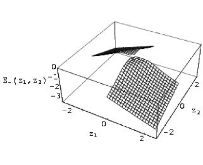
Figure 1: $E_{-}^{R}(z_{1},z_{2})$ for an inhomogeneous field over all space plotted for systems in which the particles are on opposite sides of the origin. The system could be represented by a point in the near quadrant, in which case $z_{1}>0$ and $z_{2}<0$. If particle 1 and particle 2 are interchanged, then the system would be represented by a point in the far quadrant obtained by a reflection across the line $z_{1}=z_{2}$. For $E_{-}^{R}$ the energy is monotonically decreasing as either particle moves away from the origin and there is no stable state. All the energies are scaled by $E_{0}=\mu B_{0}$ and the coordinates are scaled by $r_{0}$ which is defined by $E_{0}=2f(r_{0})\Leftrightarrow r_{0}=(2\mu/B_{0})^{1/3}$.

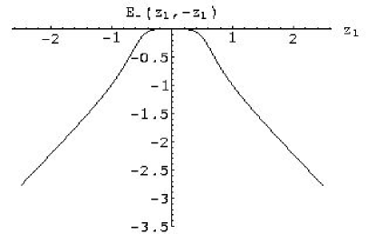
Figure 2: $E_{-}^{R}(z_{1},-z_{1})$ for an inhomogeneous field over all space. This is the same as the contour with $z_{1}+z_{2}=0$ in the FIG. 1.

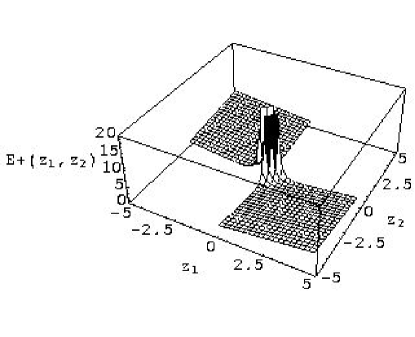
Figure 3: The positive eigenvalue $E_{+}^{R}(z_{1},z_{2})$ for an inhomogeneous field over all space. We see stable states can occur in this case.

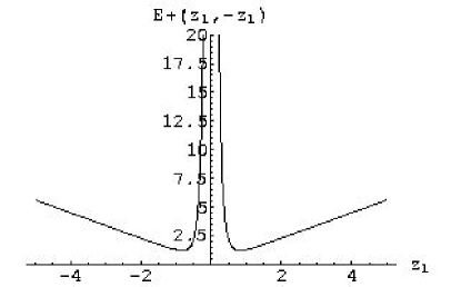
Figure 4: $E_{+}^{R}(z_{1},-z_{1})$ for an inhomogeneous field over all space. The rapid increase is due to the divergence of the dipole-dipole potential.

It is interesting to determine the nature of the spin wavefunctions for $\left|\pm a\right\rangle$ for large and small values of separation $r$ when a magnetic field is present. For large $r(z>0)\Leftrightarrow r\rightarrow\infty\ (\sin\omega\rightarrow-1)$:

$$\left|-a\right\rangle \rightarrow \frac{1}{\sqrt{2}}(\left|T\right\rangle+\left|S\right\rangle)=\left|+\right\rangle_{1}\left|-\right\rangle_{2},$$ (45)

$$E_{-}^{R} \rightarrow -gr,$$ (46)

$$\left|+a\right\rangle \rightarrow \frac{1}{\sqrt{2}}(\left|T\right\rangle-\left|S\right\rangle)=\left|-\right\rangle_{1}\left|+\right\rangle_{2},$$ (47)

$$E_{+}^{R} \rightarrow +gr$$ (48)

and for small $r\Leftrightarrow r\rightarrow 0\ (\sin\omega\rightarrow 0):$

$$\left|-a\right\rangle \rightarrow \left|S\right\rangle,\ E_{-}^{R}\rightarrow-\frac{b^{2}}{16}r^{5}$$ (49)

$$\left|+a\right\rangle \rightarrow \left|T\right\rangle,\ E_{+}^{R}\rightarrow\frac{4\mu^{2}}{r^{3}}.$$ (50)

For large separations, the energy eigenvalue is dominated by the effect of the inhomogeneous field, whereas for small separations, the eigenvalue is dominated by the dipole-dipole interaction. As the relative position $z$ of two particles goes from $-\infty$ to $0$ to $+\infty,$ the state corresponding to $\left|+a\right\rangle$ goes from an unentangled state, namely $\left|-\right\rangle_{1}\left|+\right\rangle_{2}$, to an entangled triplet $\left|T\right\rangle$ state, and then back to the unentangled $\left|-\right\rangle_{1}\left|+\right\rangle_{2}$. By superposition of states with different momenta, we could form a state that would oscillate in time between entangled and unentangled statessuper .

We need to avoid energy levels crossing each other during the application of the adiabatic perturbation. Otherwise transitions between the levels may occur. From the reduced Hamiltonian (26) one can easily find the energy levels for the other members of the triplets $\left|T_{\pm 1}\right\rangle$ to be $-2f(r)\pm 2\mu(B_{0}+bZ)$. Therefore, under the assumption that the two particles are on the opposite sides of the origin ($Z\approx 0$), we require the following equalities to avoid crossing of energy levels:

$$-2f(r)+2\mu B_{0}>E_{+}^{R}>E_{-}^{R}>-2f(r)-2\mu B_{0},$$ (51)

which are obeyed provided the energy contribution from the constant magnetic field $B_{0}$ is significantly greater than the contributions from either the inhomogeneous field or the dipole potential ($\mu B_{0}>3f(r)+g|z|/2$) condition .

Independently we also need a condition in order for the adiabatic evolution to proceed (see e.g. messiah ). Namely we need to turn on the magnetic field (inhomogeneous part) slowly, and the condition for the time period T for this switching is

$$T\gg\frac{\hbar(gz)^{2}}{(4f)^{2}\sqrt{(gz)^{2}+(2f)^{2}}}$$ (52)

or,

$$T\gg\frac{\hbar b^{2}r^{11}}{32\mu^{3}\sqrt{b^{2}r^{8}+16\mu^{2}}}.$$ (53)

Therefore the greater the separation, the more slowly the inhomogeneous field needs to be applied.

III.1 Use of Born-Oppenheimer Approximation to the Tunneling effect

So far we have neglected the kinetic term under the assumptions that the characteristic frequencies of the spin precession are much greater than those of the translational motion of the two particles. These assumptions are strictly true, for instance, for the NMR case where particles are part of the molecules and hence they are always bound.

In contrast, we want to consider a situation where the particles are essentially free. For the eigenstate $\left|+a\right\rangle$, a graph of the corresponding eigenvalue $E_{+}^{R}(z)$ is a positive double hump function which describes two bound particles, one on either side of the origin. The potential permits tunneling across the barrier. In this tunnelling process the two particles would be exchanged. First we note that the Schrodinger equation for the center of mass motion as well as the relative motion is invariant under the transformation $z_{1}\rightarrow z_{2}$ and $z_{2}\rightarrow z_{1}$ which corresponds to the tunneling transition. In $(z_{1},z_{2})$ space, this transformation corresponds to a reflection across the line $z_{1}=z_{2}$. The corresponding states are degenerate in energy. The Hamiltonian is also invariant under the parity transformation $z_{1}\rightarrow-z_{1}$, $z_{2}\rightarrow-z_{2}$.

In order to analyze this process, we can utilize a Born-Oppenheimer approximation and we can separate two degrees of freedom by the use of an average potential in the Schrodinger equation for the relative motion of the particles. Thus the problem is reduced to a one body problem with the potential for the relative coordinates. The appropriate potential is in fact the energy eigenvalue $E_{+}^{R}(z)$ which was obtained in the previous section:

$$V(z)=E_{+}^{R}(z)=\frac{2\mu^{2}}{|z|^{3}}+\sqrt{g^{2}z^{2}+\frac{4\mu^{4}}{z^{6}}}.$$ (54)

Therefore this approximation yields:

$$H_{BO}\left|E\right\rangle = E\left|E\right\rangle$$ (55)

$$H_{BO} = \frac{p^{2}}{m}+E_{+}^{R}(z).$$ (56)

As is usual for the singular potential $\propto r^{-n}$ ($n>2$) the barrier becomes infinitely high at the origin. To estimate the tunneling probability we introduce a cutoff for small $r$ defined by $r_{c}$. Figure 5 shows a typical shape of the potential barrier after this regularization.

Figure 5: Potential energy barrier $E_{+}^{R}(z=z_{1}-z_{2})$ after the regularization.

Since the Hamiltonian (56) commutes with the parity operator, the eigenstates of it are also eigenstates of the parity, namely they are either symmetric or antisymmetric. Let us denote these states by $|\phi_{S}\rangle$ and $|\phi_{A}\rangle$ respectively. Then in general we know $E_{S}\leq E_{A}$, where $E_{S}$ ($E_{A}$) is the eigenvalue of $|\phi_{S}\rangle$ ($|\phi_{A}\rangle$). Now we consider a state in which the particle is located on either the right side of the barrier or the left side and express these states by $|\phi_{R}\rangle$ and $|\phi_{L}\rangle$ respectively. Notice that they are not eigenstates of the Hamiltonian (56) in general. Obviously we have the following relation:

$$|\phi_{S}\rangle = \frac{1}{\surd{2}}(|\phi_{R}\rangle+|\phi_{L}\rangle)$$ (57)

$$|\phi_{A}\rangle = \frac{1}{\surd{2}}(|\phi_{R}\rangle-|\phi_{L}\rangle)$$ (58)

up to a phase factor. Therefore if we choose the initial state at $t=0$ as $|\phi_{R}\rangle$, then after simple calculations we get the state at time $t$ as follows.

$$|\phi_{R}(t)\rangle\propto\cos(\frac{\Delta t}{\hbar})|\phi_{R}\rangle+i\sin(\frac{\Delta t}{\hbar})|\phi_{L}\rangle,$$ (59)

where $\Delta=(E_{A}-E_{S})/2$ and we omit an overall time dependent phase factor which is irrelevant right now. Therefore we observe that the state is oscillating between a configuration in which the particle is on the right side and a configuration in which the particle is on the left side. In terms of the original variables, the positions of two particles are being exchanged in time.

To know the characteristic frequency $\Delta/\hbar$ we need to know the eigenvalues and the states of the Hamiltonian using the relation $\Delta=-\langle\phi_{R}|H_{BO}|\phi_{L}\rangle$. This requires knowledge about the solution to the Schrodinger equation (55). Instead we can use the WKB approximation to examine the possibility of this effect.

Using the WKB method we calculate the probability $w$ for a particle at rest around one minima $r_{m}$ of the potential to tunnel across the potential barrier to the other minimum:

$$w(E=0)\simeq\exp\left[-8\sqrt{\frac{m\mu^{2}}{\hbar^{2}}}(\frac{3}{\sqrt{r_{c}}}-\frac{2}{\sqrt{r_{m}}})\right].$$ (60)

A cutoff distance of $10^{-15}m$ was chosen for $r_{c}$, approximately the Compton wavelength of the neutron. This value for $r_{c}$ and the value of $r_{m}$ from Appendix B yields an estimate for $w\sim e^{-0.94}\sim 0.39$. It suggests a possibility of the tunneling effect, namely, the exchanging of the two particles through the barrier. We summarize these calculations in Appendix B.

Two remarks are in order: when the potential barrier becomes infinite the ground state will be degenerate ($E_{S}=E_{A}\Leftrightarrow\Delta=0$). This means there are no oscillations at all. And hence there exist the states $|\phi_{R}\rangle$ and $|\phi_{L}\rangle$ separately. Although these states are not eigenstates of the parity operator, because of the degeneracy they are allowed states. This is an example of the spontaneous symmetry breaking. To examine the possibility of the exchanging effect more precisely we also need to include the hyperfine interaction term in the original potential (2), which becomes important at short distances.

IV Case 2: Magnetic field present on the right side of the origin only

We assume the magnetic field $B(z)$ is in the $z$-direction and that it is non-zero only in some region on the right side of the origin ($z_{1},z_{2}>0$). Outside of this region, for example on the left, the magnetic field vanishes so, for example, $B(z_{1})\psi_{L}(z_{1})=0$, $B(z_{2})\psi_{L}(z_{2})=0,$ etc. This magnetic field breaks the translational symmetry of the field present in Case 1. Using these properties we can show that

$$\Sigma_{+}\left|S\right\rangle=\Sigma_{+}\left|T\right\rangle=0$$ (61)

$$\Sigma_{-}\left|S\right\rangle = -B_{T}\left|T\right\rangle$$ (62)

$$\Sigma_{-}\left|T\right\rangle = -B_{T}\left|S\right\rangle$$ (63)

where we define

$$B_{T}(z_{1},z_{2})=B(z_{1})+B(z_{2}).$$ (64)

Note that for our model, either particle 1 or 2 will be on the left side of the origin so either $B(z_{1})$ or $B(z_{2})$ will vanish. Thus for the special case of a constant field $B_{0}$ on the right side, we have $B_{T}=B_{0}.$ With our assumptions we can express $B_{T}(z_{1},z_{2})$ in the following way:

$$B_{T}(z_{1},z_{2})=B(z_{1})\theta(z_{1}-z_{2})+B(z_{2})\theta(z_{2}-z_{1})$$ (65)

In the impulsive approximation, these results yield a representation of $H_{I}$ using the basis states $\{\left|T\right\rangle,\left|S\right\rangle\}$

$$H_{I}=\mu B_{T}\left[\begin{array}[]{cc}0&1\\ 1&0\end{array}\right].$$ (66)

We notice that the $B_{T}$ field causes transitions between the singlet and triplet states like the inhomogeneous field in all space. This suggests that even the simplest case (a constant field $B_{0}$ on the right side) will do this. This transition might be of interest, in particular, in applications of quantum computation. Similar discussion were done by several authors (see Ref. unanyan and references therein). However, the transition between the singlet and the triplet was not discussed in there.

The remaining components of the triplet also transform among themselves, which follows from:

$$\Sigma_{+}\left|T_{\pm 1}\right\rangle = \pm B_{T}\left|T_{\pm 1}\right\rangle$$ (67)

$$\Sigma_{-}\left|T_{\pm 1}\right\rangle = 0.$$ (68)

The interaction Hamiltonian in the basis {$\left|T_{-1}\right\rangle,\left|T_{1}\right\rangle$ } is:

$$H_{I}=\mu B_{T}\left[\begin{array}[]{cc}1&0\\ 0&-1\end{array}\right]$$ (69)

In terms of the basis $\{\left|T_{-1}\right\rangle,\left|T_{1}\right\rangle,\left|T\right\rangle,\left|S\right\rangle\}$ , the total reduced Hamiltonian $H^{R}$ can therefore be written as

$$H^{R}=f(r)\left[\begin{array}[]{cccc}-2&0&0&0\\ 0&-2&0&0\\ 0&0&4&0\\ 0&0&0&0\end{array}\right]+\mu B_{T}\left[\begin{array}[]{cccc}1&0&0&0\\ 0&-1&0&0\\ 0&0&0&1\\ 0&0&1&0\end{array}\right].$$ (70)

After applying the magnetic field perturbation, the $\left|T_{-1}\right\rangle$ and $\left|T_{1}\right\rangle$ components still do not mix with any other components. The total reduced Hamiltonian is diagonal in the subspace spanned by $\left|T_{-1}\right\rangle$ and $\left|T_{1}\right\rangle,$ and the corresponding energy eigenvalues are $E_{-1}^{R}=-2f+\mu B_{T}$ and $E_{1}^{R}=-2f-\mu B_{T}$.

We now consider in detail the subspace spanned by $\left|T\right\rangle,\left|S\right\rangle$ which is not diagonal. In the same manner as in the previous section we express the total reduced Hamiltonian $H_{2}^{R}$ in terms of the Pauli matrices as:

$$H_{2}^{R}=2f(r)\bm{I}+\bm{\alpha}\cdot\bm{\sigma}$$ (71)

where the vector $\bm{\alpha}$ $=(\mu B_{T},0,2f)$. Define the angle $\theta$ by

$$\tan\theta=\frac{\alpha_{x}}{\alpha_{z}}=\frac{\mu B_{T}(z_{1},z_{2})}{2f}=\frac{B_{T}r^{3}}{2\mu}$$ (72)

and the quadrant is specified by

$$\sin\theta=\frac{\mu B_{T}}{\sqrt{\mu^{2}B_{T}^{2}+4f^{2}}}.$$ (73)

Solving for the eigenvectors and eigenvalues of $H_{2}^{R}$, we obtain

$$\left|-a\right\rangle = -\sin\frac{\theta}{2}\left|T\right\rangle+\cos\frac{\theta}{2}\left|S\right\rangle,$$ (74)

$$E_{-}^{R} = 2f-|\bm{\alpha}|=2f(1-\sec\theta)$$ (75)

and

$$\left|+a\right\rangle = \cos\frac{\theta}{2}\left|T\right\rangle+\sin\frac{\theta}{2}\left|S\right\rangle,$$ (76)

$$E_{+}^{R} = 2f+|\bm{\alpha}|=2f(1+\sec\theta).$$ (77)

To avoid the crossing of energy levels, we require $E_{-}^{R}>E_{-1}^{R}$ which implies that

$$2\mu B_{T}<3f(r).$$ (78)

And also from the adiabatic theorem we get

$$T\gg\frac{\hbar(\mu B_{T})^{2}}{(4f)^{2}\sqrt{(\mu B_{T})^{2}+(2f)^{2}}}.$$ (79)

Using the above condition (78) we estimate the lower limit of the time $T_{min}$ as

$$T_{min}\sim\frac{9}{80}\frac{\hbar}{f(r)}\simeq 0.11\hbar f^{-1}.$$ (80)

The restriction of Eq. (78) severely limits possible modulation frequencies of the field being applied adiabatically. We briefly mention a procedure, similar to that used in Case 1, which results in a much larger bandwidth. We first apply the large constant $B_{0}$ field impulsively over all space impulsive . Then we apply the inhomogeneous field adiabatically over the right side only. With this procedure, the restriction on the energy levels to avoid crossings is similar to Eq. (51), but the levels $|T_{-1}\rangle$ and $|T_{+1}\rangle$ are also shifted by the inhomogeneous field $\pm\mu B_{T}|_{B_{0}=0}$. The quantity $\mu B_{T}|_{B_{0}=0}$ is always positive since the inhomogeneous field is on the right side, so the requirement for no level crossing is less stringent, and is met simply if $\mu B_{0}>4f$. The corresponding requirement for the validity of the adiabatic approximation is the same as Eq. (53), with $r$ replaced by the positive value of the pair $\{z_{1},z_{2}\}$.

IV.1 Homogeneous field on the right side only

We can consider several different magnetic field strengths $B_{T}(z_{1},z_{2}).$  For the simplest case, in which $B_{T}$ is a constant on the right side, we find that $E_{-}^{R}(z_{1},z_{2})$ is a negative potential (Figures 6–7) that does not confine the particles so no stable states are expected, while $E_{+}^{R}(z_{1},z_{2})$ is a positive potential that also does not confine particles (Figures 8–9).

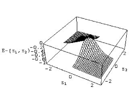
Figure 6: $E_{-}^{R}(z_{1},z_{2})$ for a constant magnetic field on the right side, plotted for particles on opposite sides of the origin.

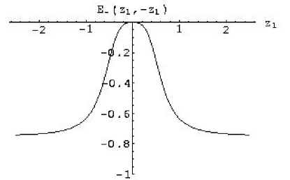
Figure 7: $E_{-}(z1,-z1)$ for a constant magnetic field This curve is obtained by plotting the function $E_{-}(z1,z2)$ for the contour $z1+z2=0$ .

Figure 8: $E_{+}(z1,z2)$ for a constant magnetic field on the right, plotted only for particles on opposite sides of the origin.

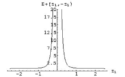
Figure 9: $E_{+}(z1,-z1)$ plotted for a constant magnetic field on the right side of the origin.

IV.2 Inhomogeneous field on the right side only

Next we shall consider an inhomogeneous field ($B_{T}=B_{0}+bZ+br/2$) on the right side. The graphs for $E_{-}^{R}(z_{1},z_{2})$ (FIG. 10–11) are plotted with the same parameters as FIG. 1–4 for the comparison. Similar results are obtained in this case.

The positive energy $E_{+}^{R}(z_{1},z_{2})$ has a double hump structure (FIG. 12–13) with two potential wells for quasi-bound states separated by an energy peak. We note that unlike in case 1, there is no symmetry with respect to reflection across the line $z_{1}+z_{2}=0$ so the forces acting on the particles are not equal. The force due to the magnetic field acts only on the particle on the right side. Here we define the effective forces through partial differentiations of the effective potentials $E_{\pm}^{R}$ with respect to $z_{1}$ and $z_{2}$.

Figure 10: $E_{-}(z1,z2)$ for an inhomogeneous field on the right side, plotted for particles on opposite sides of the origin. All parameters for the FIG. 10–13 are chosen same as for FIG. 1–4.

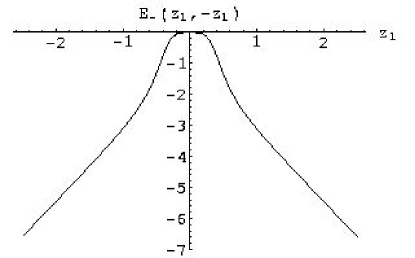
Figure 11: $E_{-}(z1,-z1)$ for an inhomogeneous field on the right side only.

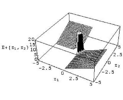
Figure 12: $E_{+}(z1,z2)$ for an inhomogeneous field on the right side, plotted for particles on opposite sides of the origin.

Figure 13: $E_{+}(z1,-z1)$ for an inhomogeneous field on the right side.

IV.3 Summary

In summary, with the adiabatic evolution of spins when we apply the magnetic field on the right side, we find that the initial singlet ground state singlet $\left|S\right\rangle$ has evolved into the eigenstate given by a linear combination of singlet and triplet states:

$$\left|-a\right\rangle=-\sin\frac{\theta}{2}\left|T\right\rangle+\cos\frac{\theta}{2}\left|S\right\rangle.$$ (81)

In this adiabatic evolution, the reduced energy goes from $0$ for $\left|S\right\rangle$ to $2f(1-\sec\theta)$ for $\left|-a\right\rangle$. Since $\left|-a\right\rangle$ is a spin eigenstate of the total Hamiltonian, there is an overall time dependent phase factor, $e^{-iE_{-}^{R}t/\hbar}$ for this state, which we have omitted.

The eigenstates $\left|\pm a\right\rangle$ have the property that, for any value of $\theta$, the spins of the particles in the $z$-direction are always correlated:

$$(S_{z_{1}}+S_{z_{2}})\left|\pm a\right\rangle=0.$$ (82)

This result, which follows since $[H_{T},S_{z_{1}}+S_{z_{2}}]=0$, indicates that the spins of the two particles remain correlated if an inhomogeneous magnetic field is applied only to the particle on the right side of the origin.

V Computation of the density matrix for an adiabatic change in the magnetic field on the right side only

In this section we shall study the case 2 further in detail. One convenient way to consider the effect of the magnetic field (which is present only on the right side) on the state of the system on the left side (where the magnetic field vanishes) is to predict the results of a measurement of an observable $A$ which is defined only on the left side. The predictions can be done by means of the reduced density matrix $\rho(L,-a)$ on the left side $L$ for the state $\left|-a\right\rangle$density :

$$\rho(L,-a)=Tr_{right\text{ }side}\left|-a\right\rangle\left\langle-a\right|.$$ (83)

In order to compute this reduced density matrix for $\left|-a\right\rangle$, we first compute the reduced density matrices for the basis states $\left|S\right\rangle$ and $\left|T\right\rangle$.  For an observable $A$ which is defined only on the left side we have $A\psi_{R}(z_{2})=0$, etc. The result of a measurement of $A$ for the state $\left|T\right\rangle$ is defined as

$$Tr\rho(L,T)A=\left\langle T\right|A\left|T\right\rangle$$ (84)

and can be computed using the expression for $|T\rangle$:

$$\langle T|A|T\rangle = \frac{1}{4}[{}_{1}\langle+L|A|+L\rangle_{1}+{}_{1}\langle-L|A|-L\rangle_{1}$$ (86)

$$\ +{}_{2}\langle-L|A|-L\rangle_{2}+{}_{2}\langle+L|A|+L\rangle_{2}]$$

where we have defined

$$\left|\pm L\right\rangle_{1} \equiv \left|\pm\right\rangle_{1}\psi_{L}(z_{1})$$ (87)

$$\left|\pm L\right\rangle_{2} \equiv \left|\pm\right\rangle_{2}\psi_{L}(z_{2}).$$ (88)

The corresponding reduced density matrix on the left side is

$$\rho(L,T) = \frac{1}{4}[|+L\rangle_{1}{}_{1}\langle+L|+|-L\rangle_{1}{}_{1}\langle-L|$$ (90)

$$\ +|+L\rangle_{22}\langle+L|+\text{\ }|-L\rangle_{22}\langle-L|].$$

By a similar calculation we find that the reduced density matrix for $\left|S\right\rangle$ has the same value as for $\left|T\right\rangle$:

$$\rho(L,S) = Tr_{rightside}\left|S\right\rangle\left\langle S\right|$$ (91)

$$= \rho(L,T).$$ (92)

We also compute

$$\rho(L,TS) = Tr_{rightside}|T\rangle\langle S|$$ (93)

$$= \frac{1}{4}[|+L\rangle_{1}{}_{1}\langle+L|-|-L\rangle_{1}{}_{1}\langle-L|$$ (95)

$$\ +|+L\rangle_{2}{}_{2}\langle+L|-|-L\rangle_{2}{}_{2}\langle-L|]$$

and find that

$$\rho(L,TS)=\rho(L,ST).$$ (96)

Using the preceding results, we can write an expression for $\rho(L,-a)$ using the definition of the state $\left|-a\right\rangle$:

$$\rho(L,-a) = \sin^{2}\frac{\theta}{2}\rho(L,T)+\cos^{2}\frac{\theta}{2}\rho(L,S)$$ (97)

$$-2\sin\frac{\theta}{2}\cos\frac{\theta}{2}\rho(L,TS)$$

$$= \rho(L,S)-\rho(L,TS)\sin\theta.$$ (98)

This last result can be written in matrix form in the basis {$\left|+L\right\rangle_{1},\left|-L\right\rangle_{1},\left|+L\right\rangle_{2},\left|-L\right\rangle_{2}\}:$

$$\rho(L,-a)=\frac{1}{4}\left[\begin{array}[]{cccc}1-\sin\theta&0&0&0\\ 0&1+\sin\theta&0&0\\ 0&0&1-\sin\theta&0\\ 0&0&0&1+\sin\theta\end{array}\right].$$ (99)

One can contemplate making standard quantum mechanical measurements in which a superposition collapses to a eigenstateperesbook . Alternatively we consider the use of a protective Stern-Gerlach measurement, in which there is an adiabatic interaction between the pointer and the systemav ; aavwave ; aavprotec . We want to examine the possibility of the protective measurement in our model under the assumption we will work in a decoherence free subspace. In previous discussions of protective measurements, only the case of a small perturbation was considered in order to minimize the change in the wavefunction of the state to be measured. In our system, such restrictions are not necessary. As long as the interaction is adiabatic, the state will evolve continuously as an eigenstate of the instantaneous Hamiltonian, without any transition provided there is no degeneracy in the energy. If the magnetic field is applied adiabatically, the field can become large, resulting in a large change in the wavefunction. Because the changes are adiabatic, they are reversible as the magnetic field is reduced. Since a protective measurement of the spin for our two particle system does not change the state of the system, the protective measurement does not end the entanglement.

In the spin-spin model, the states $\left|-a\right\rangle$ and $\left|+a\right\rangle$ into which $\left|S\right\rangle$ and $\left|T\right\rangle$ evolve when a magnetic field is applied on the right side are non-degenerate so a protective measurement of the reduced density matrix should be possible. Indeed all four basis states$\left|-a\right\rangle$, $\left|+a\right\rangle$, $\left|T_{1}\right\rangle$, and $\left|T_{-1}\right\rangle$ are non-degenerate provided $f\neq 0$ and $B\neq 0$ so a protective measurement should be possible of the density matrixanandanden . As a consequence the result of a protective measurement of an observable $A$ that acts only on the left side can be written as the trace over the reduced density matrix:

$$<A>_{(L,-a)}=Tr(\rho(L,-a)A).$$ (100)

Note that here $<A>$ represents the result of a single protective measurement on a single system. It does not have the usual meaning of the expectation value of $A$, which is based on the measurement of the observable $A$ for an ensemble of identically prepared systems. Since the elements of the density matrix depend on $\theta$, it is clear that changes in $\theta$, resulting from either changes in $B$ or ($z_{1}-z_{2})$, will affect the measured values of observables $A$. In other words, in this model with a finite separation, by changing the value of the magnetic field on the right side, it is possible to detect the effect on the left side nonlocally. Note that nowhere do we use the specific form of the potential. Indeed, we could use the formalism presented with any function of the separation.

To illustrate the application of a protective measurement, we could measure the total spin in the z- direction for both particles using local measurements on the left side only. We assume we use a Stern-Gerlach analyzer with an inhomogeneous field in the $z$-direction and we observe the deflection of the wave packet corresponding to a particle. We assume we have calibrated our apparatus so that we can determine the spin of a particle on the left side by observation of the deflection in the $z$- direction at a certain point in the experiment. Since the particles are indistinguishable, a single protective measurement of the spin of a particle on the left will yield a deflection corresponding to the result

$$\left\langle S_{z_{1}}+S_{z_{2}}\right\rangle_{left\ side}=tr(\rho[S_{z_{1}}+S_{z_{2}}])=-\frac{1}{2}\sin\theta$$ (101)

where the value of $\theta$ is determined by the magnetic field on the right side and the distance between the particles. The corresponding total spin in the $z$-direction measured on the right side is $\frac{1}{2}$sin$\theta$. Since this protective measurement has not collapsed the wave function, we could do additional measurements on the same state to determine the rest of the density matrix $\rho_{(L,-a)}$ in the $\left|T\right\rangle,\left|S\right\rangle$ subspace. If we used Stern-Gerlach analyzers with fields in the $x$ and $y$ directions for two additional experiments, respectively, we would find:

$$\left\langle S_{x_{1}}+S_{x_{2}}\right\rangle_{left\ side}\ =\left\langle S_{y_{1}}+S_{y_{2}}\right\rangle_{left\ side}=0.$$ (102)

These components of the spin vanish because we chose the magnetic field on the right side to be in the $z$-direction.

It is interesting to contrast the protective measurement of $S_{z_{1}}+S_{z_{2}}$ with the ordinary measurements. In an standard quantum mechanical measurement the wavefunction collapses and an eigenvalue of the operator is measured. To determine the expectation value of the operator, one needs to make a statistically significant number of measurements on an ensemble of identically prepared systems. In our model, since the particles are indistinguishable, for each standard measurement on a different identically prepared system, a deflection in the Stern-Gerlach apparatus will be measured that corresponds to spin of $+\frac{1}{2}$ or $-\frac{1}{2}$. If enough measurements are done, it will be determined that the probability of measuring $+\frac{1}{2}$ is $\frac{1}{2}(1-\sin\theta)$ and the probability of measuring $-\frac{1}{2}$ is $\frac{1}{2}(1+\sin\theta)$. Using these probabilities, the standard measurements will determine that the expectation value of the operator $S_{z_{1}}+S_{z_{2}}$ on the left side is $-\frac{1}{2}\sin\theta,$ in agreement with the single protective measurement.

This comparison of the two methods illustrates some of the advantages of protective measurements and some of the disadvantages of standard measurements.

VI CONCLUSION AND DISCUSSIONS

A system was considered in which two neutral spin 1/2 particles interact through a diple-dipole potential. The potential leads to singlet and triplet entangled states which are modified when we apply a magnetic field over all space (Case 1), or over just the region to the right of the origin (Case 2).

For the case 1 we showed that the singlet state is essentially unstable and it tends to separate. However, the spin zero component of the triplet will have a double hump shape energy which implies the particles will tend to stay near the minima with high probabilities and form a bound state. Also we showed that it is possible to have a tunneling effect in this case. Such an effect might have applications in quantum computation.

For the case 2 we observed that although the external field is applied only in one part of the system, the other part will be affected by it due to the entanglement of the system. This manifests the nonlocality of the entanglement in quantum mechanics. It appears protective measurements can be used to determine the density matrix without ending the entanglement. As discussed above for the case of finite separation, one limitation in the signaling between the two regions of space in this model lies in the requirement that we must have an adiabatic perturbation or transitions will occur between states. When the magnetic field is turned on, it must be done slowly enough so that no transitions are induced between the initial state and other states. Although the specific restrictions depend on the manner in which the perturbations are applied, they require that the potential due to the dipole-dipole interaction does not vanish.

Appendix A Model with confining potentials

In this appendix we will examine our model with additional confining potentials (for instance, created by the optical laser). For simplicity we approximate this potential by a harmonic potential around certain point $\bm{x}_{0}$ with characteristic frequency $\Omega$, namely, $V(\bm{x})=\frac{1}{2}m\Omega^{2}(\bm{x}-\bm{x}_{0})^{2}$. We choose the center of the potential in such a way that two particles will be separated by a distance $z_{0}$. Under these conditions the ground state energy of the particles is $\frac{3}{2}\Omega$ (we use $\hbar=1$ in appendices.) and the corresponding states are

$$\psi_{R}(\bm{x}_{i}) = (\frac{\xi}{\pi})^{\frac{3}{4}}e^{-\frac{1}{2}\xi(x_{i}^{2}+y_{i}^{2}+(z_{i}-\frac{z_{0}}{2})^{2})}$$ (103)

$$\psi_{L}(\bm{x}_{i}) = (\frac{\xi}{\pi})^{\frac{3}{4}}e^{-\frac{1}{2}\xi(x_{i}^{2}+y_{i}^{2}+(z_{i}+\frac{z_{0}}{2})^{2})},$$ (104)

for $i=1,2$ and the parameter $\xi=\sqrt{m\Omega}$ is introduced. To have a stable ground state in our model we require the energy levels are well separated, or the parameter $\xi$ is large. (Similarly we can assign these wave packets for the free particles case too.) After we obtain the spatial wave functions for the singlet and the triplets comment2 , we can estimate the effect of the hyperfine interaction term in the dipole-dipole potential (2). We evaluate the expectation values of the delta function as follows.

$$\langle\delta(\bm{x})\rangle_{S} = 4(\frac{\xi}{2\pi})^{\frac{3}{2}}(1+e^{\frac{1}{2}\xi z_{0}^{2}})^{-1},$$ (105)

$$\langle\delta(\bm{x})\rangle_{T} = 0.$$ (106)

Therefore, under our assumptions the contribution from the hyperfine interaction is negligible in our model because of the exponential factor in (105). However, in contrast, this term plays an important role in a situation where the distance becomes very small and we need to add this contribution too. This regime is discussed in the literature, for instance, see Ref. you and references therein.

Next we estimate the change in the positions of the particles and the kinetic energy of them. From simple calculations it is easy to see that the expectation values of the relative position and the center of mass are zero. Similarly we obtain for the expectation value for the center of mass kinetic energy

$$\left\langle\frac{P^{2}}{2m}\right\rangle_{S}=\left\langle\frac{P^{2}}{2m}\right\rangle_{T}=\frac{\xi}{2m}$$ (107)

and for the relative kinetic energy we have

$$\left\langle\frac{p^{2}}{m}\right\rangle_{S} = \frac{\xi}{4m}(1-\frac{\xi z_{0}^{2}}{e^{\frac{1}{2}\xi z_{0}^{2}}+1})$$ (108)

$$\left\langle\frac{p^{2}}{m}\right\rangle_{T} = \frac{\xi}{4m}(1+\frac{\xi z_{0}^{2}}{e^{\frac{1}{2}\xi z_{0}^{2}}-1}).$$ (109)

Again, the second term inside the parenthesis is negligible by our assumptions. And hence we see that the corrections due to the motion of the particles are small.

Appendix B Calculation of the tunneling probability (60)

To estimate the tunneling probability we simplify our model as follows. First we calculate the minima $r_{m}$ of the potential (54), this is easily found

$$gr_{m}=2\sqrt{15}f(r_{m})\Leftrightarrow r_{m}=(\frac{240\mu^{2}}{b^{2}})^{\frac{1}{8}}.$$ (110)

Then we evaluate the the tunneling probability between two minima through the dipole-dipole interaction barrier assuming that the potential is mainly dominated by this interaction in small distance. We use the WKB method landau to get the probability $w(E)$ for the particle with the kinetic energy $E=k^{2}/m$ (the mass is $m/2$), that is,

$$w(E)\simeq\exp[-2\left|\int_{-r_{m}}^{r_{m}}\sqrt{m(V(z)-E)}\ dz\right|\ ].$$ (111)

In our case the simplified potential is $V(z)=4\mu^{2}/|z|^{3}$. As we mentioned earlier we introduce the cutoff at $r_{c}$ to get rid of the divergent integral. Under these assumptions and defining the momentum $k_{m}$ and $k_{c}$ corresponding to the minima and the cutoff respectively, i.e. $k_{m}^{2}/m=V(r_{m})$ and $k_{c}^{2}/m=V(r_{c})$, the integral inside the exponent of (111) is evaluated as below.

$$-2\sqrt{k_{m}^{2}-k^{2}}\ r_{m}-kr_{m}(\frac{k_{m}}{k})^{\frac{1}{3}}B_{\frac{5}{6},\frac{1}{2}}(\frac{k}{k_{m}})+3\sqrt{k_{c}^{2}-k^{2}}\ r_{c},$$ (112)

where $B_{a,b}(x)$ is the incomplete beta function defined by $B_{a,b}(x)=\int_{0}^{x}t^{a-1}(1-t)^{b-1}dt$ and we neglect the positive orders of $r_{c}$ (in $r_{c}/r_{m}\ll 1$ limit). Therefore for the rest particle ($k=0$) at the minima, a rough estimate for the tunneling probability is

$$w(E=0)\simeq\exp[-4(3k_{c}r_{c}-2k_{m}r_{m})]$$ (113)

which is given in the text after substituting $k_{m}$ and $k_{c}$. Another case is for the particle having the minimum potential energy ($k=k_{m}$):

$$w(E=V(r_{m}))\simeq\exp[-4(3k_{c}r_{c}-B(\frac{5}{6},\frac{1}{2})k_{m}r_{m})]$$ (114)

where $B(\frac{5}{6},\frac{1}{2})\simeq 2.24$ is the usual beta function. And hence we see that this is the same order as (113).

References

- (1) For a general reference, see for instance, M. A. Nielsen and I. L. Chuang, Quantum Computation and Quantum Information, Cambridge University Press (2000).
- (2) L. You and M. S. Chapman, Phys. Rev. A 62, 052302 (2000).
- (3) R. G. Unanyan, N. V. Vitanov, K. Bergmann, Phys. Rev. Lett. 87, 137902 (2001).
- (4) Y. Aharonov, J. Anandan, L. Vaidman, Found. Phys. 26, 117-126 (1996).
- (5) Y. Aharonov, J. Anandan, L. Vaidman, Phys. Rev. A 47, 4616-4626 (1993).
- (6) J. Anandan and Y. Aharonov, Found. Phys. Lett. 12, 571-578 (1999).
- (7) A. Messiah, Quantum Mechanics, Vol. 2, North-Holland Publishing, Amsterdam, 739-759 (1963).
- (8) Strictly speaking the magnetic field must satisfy the Maxwell equations, i.e., and (without external currents). In our case the simplest realistic inhomogeneous field might be chosen as which satisfies the Maxwell equations. This choice of the field and the assumption yields the same result as obtained by our choice (21). See also the discussions in Ref. anandandivB
- (9) This application of the field eliminates the non-level crossing condition (51). On the other hand, if we apply both parts of the magnetic field adiabatically, we will have more restrictive condition which limits the capabilities of our model.
- (10) J. Anandan, Found. Phys. Lett. 6, 503-532 (1993).
- (11) We can imagine two identical particles moving toward each other which are represented by Gaussian wave packets which are superpositions of the different momenta of the plane waves. The time development of this system is similar to the one discussed in the text after eq. (59).
- (12) This sufficient condition is obtained by using the inequality and .
- (13) L. D. Landau and E. M. Lifshitz, Quantum Mechanics, Butterworth-Heinemann (1981).
- (14) The validity of this impulsive approximation is guaranteed by an equality messiah .
- (15) Similarly we can evaluate the reduced density matrix for the state and it is found to be .
- (16) A. Peres, Quantum Theory: Concepts and Methods, Kluwer Academic Publishers, Dorthecht, Netherlands (1995)
- (17) Y. Aharonov, L. Vaidman, Phys. Lett. A 178, 38-42 (1993).
- (18) The spatial wave functions for the singlet and the triplets would not be normalized by the factor if we use these wave packets (103,104). This is because there is overlapping of two wave packets. And we need to renormalize the spatial wave functions after forming (4). Therefore these wave packets are approximated trial wave functions.