Quantum chaos in elementary quantum mechanics

Abstract

We introduce an analytical solution to the one of the most familiar problems from the elementary quantum mechanics textbooks. The following discussion provides simple illustrations to a number of general concepts of quantum chaology, along with some recent developments in the field and a historical perspective on the subject.

I Introduction

Many aspects of the behavior of quantum systems can be understood and interpreted in terms of the dynamical characteristics of their classical counterparts. It is often possible to obtain quantitatively such important attributes of a quantum system as its spectra and even its wave function in terms of the appropriate classical quantities Gutzw ; Cvit ; Kay . Although the main objects of the classical dynamics, the dynamical trajectories, are not something that can be rigorously used in the context of quantum mechanics, they can often facilitate our understanding of quantum realm, by providing means for semiclassical interpretation.

As an illustration of this point, let us first look at the infinite square well problem. Let us consider a particle confined in the infinite square well potential,

$$V(x)=\cases{0,&if $0<x<b$,\cr\infty&if $x\leq 0$ or $x\geq L$.\cr}$$ (1)

Classically, the dynamics of such particle is as simple as it can possibly be - the particle simply bounces periodically between the two walls. Geometrically its trajectory is a closed loop, which the particle traverses over and over again. The total length of the loop is twice the width of the well, ${\cal L}=2L$, and the period of motion is $T=2L/v$, where $v$ is the speed of the particle. As a result of the wall reflections, the momentum of the particle changes its sign, but its magnitude never changes.

Quantum mechanically, this system is nearly as simple to describe. The wave function $\psi(x)$ in this case is a combination of two plane waves,

$$\psi(x)=Ae^{ikx}+Be^{-ikx},$$ (2)

where $k=\sqrt{E}/\hbar$ is the particle’s momentum, which must satisfy the boundary conditions $\psi(0)=\psi(L)=0$. This leads to the quantization condition

$$\sin(kL)=0,$$ (3)

and hence the quantum spectrum $k_{n}$ of this problem is given by

$$L\,k_{n}=\pi n.$$ (4)

Note, that the left hand side of this equation coincides with the classical action integral,

$$S=\int_{\gamma}kdx=L\,k,$$ (5)

taken along the trajectory $\gamma$ that connects the two turning points, and hence the condition (4) implies that the action takes only discrete values, $S_{n}=\pi n$. Expressing the de Broglie wavelength $\lambda$ in terms of the momentum, $\lambda=2\pi/k$, the relationship (4) can be cast into the form ${\cal L}/\lambda_{n}=n$, which has a simple geometrical meaning. Apparently the quantization condition (4) implies that the wave (2) must fit geometrically $n$ times onto the (only) classical periodic orbit that has the length ${\cal L}$. As the energy of the particle increases, its wavelength will become smaller and smaller, however the geometrical condition ${\cal{L}}/\lambda_{n}=n$ always holds.

Such simple combination of physical and geometrical ideas were used by Bohr and his school in around 1914 to provide the first explanations to one of the most striking features of the quantum mechanical systems - the discrete nature of their energy spectra. According to their views, the discreteness of the quantum spectra turns out to be essentially a consequence of the geometrical consistency of the wave mechanics. Specifically, such “wave-geometrical” approach proved very successful in early attempts to explain the experimentally observed emission-absorption spectrum of the Hydrogen atom. In fact, the results obtained in this way were exact, and that gave serious reasons to believe that these ideas were adequate to describe the quantum physics of the subatomic world.

However, the later attempts of Bohr, Sommerfeld, van Vleck, Born and others Bohr ; VanVleck ; Born to continue the success of these ideas on more complicated atoms, failed completely. It was apparently impossible to explain even approximately the experimentally observed spectrum of the Helium atom - the next simplest atom after Hydrogen in the periodic table of elements and hence the next best candidate for a successful treatment by means of such wave-geometrical quantization. Van Vleck wrote in 1922 VanVleck :

“The conventional quantum theory of atomic structure does not appear able to account for the properties of even such a simple element as helium, and to escape from this dilemma some radical modification in the ordinary conceptions of quantum theory or of the electron may be necessary”.

What was be the nature of the difficulties that required such “radical” and “conceptual” modifications? In 1925 Max Born wrote Born :

“…the systematic application of the principles of the quantum theory… gives results in agreement with experiment only in those cases where the motion of a single electron is considered; it fails even in the treatment of the motion of the two electrons in the helium atom.

This is not surprising, for the principles used are not really consistent… A complete systematic transformation of the classical mechanics into a discontinuous mechanics is the goal towards which the quantum theory strives.”

Seemingly one makes a very simple and natural move by trying to go from the exactly solved Hydrogen atom to the Helium, by adding just one more particle to the two body nucleus-electron system of the Hydrogen. However, from the point of view of the contemporary classical mechanics, this modest generalization turns an integrable two-body system into a non-integrable three body system. Hence, in order to impose the “geometrical consistency” on the quantum waves that could describe the Helium atom in Bohr’s approach, one would have to deal with the overwhelming geometrical complexity of its classical phase space. It means that all the familiar “niceties” of the generic chaotic systems, such as the exponential proliferation of the periodic orbits associated with extreme complexity of their shapes, would have to be taken into account - something that could hardly had been done at Bohr’s time. Indeed, at the beginning of the last century chaos theory was just being developed in the works of Poincare, Lyapunov, Hadamard, Birkhoff and a few others Lyapunov ; Poincare ; Hadamard ; Birkhoff . Although the importance of the classical dynamical behavior for successful quantization was realized by certain researchers Einstein , it took about 60 years before the first semiclassical quantization procedure for nonintegrable systems was outlined. As for the Helium atom, a semiclassical quantization scheme for it was proposed in 1992 Wintgen using some recent developments of the quantum chaos theory Cvit .

II Back to 1D potential wells

Surprisingly, the difficulties of the semiclassical quantization of the classically nonintegrable Helium atom system can be illustrated by means of elementary quantum mechanics. Below we shall consider a simple modification of a completely transparent system (1) that leads to a transition from classical integrability to a non-integrability and clarifies the corresponding outburst of complexity on quantum level.

Let us add a small step at the bottom of the potential (1) and consider a point particle moving in the potential

$$V(x)=\cases{0,&if $0\leq x\leq b$,\cr V,&if $b\leq x\leq L$,\cr\infty&if $x\leq 0$ or $x\geq L$,\cr}$$ (6)

shown in Figure 1.

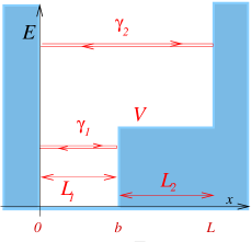
Figure 1: A simple modification of the infinite square well model - a square well with a potential step, along with the two apparent classical trajectories $\gamma_{1}$ and $\gamma_{1}$.

Seemingly the classical picture doesn’t change much. It appears that if the energy of the particle is higher than $V$, the particle will oscillate between the points $x=0$ and $x=L$ just as before, and if its energy is below the potential step hight, it will oscillate between $x=0$ and $x=b$. However, the reality turns out to be much more complicated than that.

Let us first give the quantum mechanical description of the problem. Suppose that the energy $E$ of the particle is above the potential height $V$. The momentum of the particle in the region $0\leq x\leq b$ is $k=\sqrt{E}$, and in the region $b\leq x\leq 1$ it is $\kappa=\sqrt{E-V}$, and its $\psi$ function consists of two parts,

$$\psi(x)=\cases{\sin(kx),&if $0\leq x\leq b$,\cr A\sin\left[\kappa\left(L-x\right)\right],&if $b\leq x\leq L$,\cr}$$ (7)

which match continuously at $x=b$.

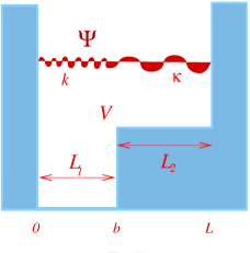
Figure 2: A quantum particle in a square well with a step.

From this continuity requirement one can determine the spectral equation for the spectrum of the problem,

$$\sin(L_{1}k+L_{2}\kappa)=r\sin\left[\left(L_{1}k-L_{2}\kappa\right)\right],\ \ \ E>V,$$ (8)

where $L_{1}=b$ and $L_{2}=L-b$ are correspondingly the lengths of the left and the right sides of the well (6) and $r$ is the reflection coefficient

$$r=\frac{k-\kappa}{k+\kappa}.$$ (9)

The $E<V$ case can be treated similarly and basically amounts to substituting $\kappa\rightarrow i\varkappa$, $\varkappa=\sqrt{V-E}$, in the expressions (8) and (9). After extracting the complex phase, the spectral equation becomes

$$\sin(L_{1}k)=\frac{(-1)^{n+1}k\left(1-e^{-2L_{2}\varkappa}\right)}{\sqrt{V\left(1+e^{-4L_{2}\varkappa}\right)+2(\varkappa^{2}-k^{2})e^{-2L_{2}\varkappa}}},\ \ \ E<V,$$ (10)

where $n=1$, $2$, …, is the root index.

There is an important analogy between (8), (10) and (3) - the arguments of the sine functions in the left hand sides of these equations are the action lengths $S(E)$ of the classically available regions in the well (6) for $E>V$ and $E<V$ correspondingly,

$$S(k)=\int_{\gamma}kdx=\cases{kL_{1}+\kappa L_{2},&if $E>V$,\cr kL_{1}&if $E<V$,\cr}$$ (11)

which is a continuous and monotonically increasing function of the energy.

On the other hand, it is interesting that unlike (3), the equations (8) for $E>V$ and (10) for $E<V$ are transcendental equations - that is substantially more difficult to solve. In fact, in absence of any analytical ways of solving the equation (8) and (10) explicitly, all the standard textbooks, e.g. Griffith ; Flugge ; Messiah ; LL , use graphical or numerical methods to approximate its roots, $k_{n}$.

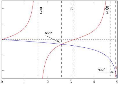
Figure 3: Typical appearance of the graphical methods currently used by the Quantum Mechanics textbooks. The roots are found as the intersection points of the graphs representing the right and the left hand sides of a suitable spectral equation, marked by the vertical dashed lines. For details see Griffith ; Flugge ; Messiah ; LL .

Notably, there are also no simple “semiclassical” interpretations similar to (4) for the results of such approximations, which, after all, does not appear important for the purpose of obtaining the numerical values for the roots of the spectral equations (8) and (10).

This is very similar to what happened to the Helium atom quantization problem - the “old quantum theory” treatment became unnecessary once the formalism of the “new” quantum mechanics of Schrödinger and Heisenberg was established and could be used. The problem of obtaining the energy spectrum of the Helium (or in principle any other atom) was reduced to a technical problem of diagonalizing the Hamiltonian matrix $H_{nm}$ by means of all sorts of numerical techniques and approximations.

Even without making any historical references, one can notice the obvious contrast in the level of complexity between the spectral equations (8), (10) and (3). What is the physical reason for it? Below we shall argue that the complexity of the spectral equations (8), (10) has a deep physical meaning and can be understood from analyzing the classical motion of a particle in the potential well (6).

III The classical limit

To start the discussion of the classical dynamics of a point particle in the potential (6), let us notice that the reflection coefficient (9) in (8) ($E>V$) does not depend on the Plank’s constant $\hbar$,

$$r=\frac{1-\sqrt{1-V/E}}{1+\sqrt{1-V/E}}.$$ (12)

Due to this circumstance this quantity (although obtained by purely quantum mechanical means LL ) is in fact quite classical, because one does not need to refer to any quantum mechanical concepts to evaluate $r$.

This curious fact can be easily interpreted and understood from general principles RS1 ; RS2 . Just as any other wave, the probability amplitude (2) gets reflected or diffracted when it encounters inhomogeneities on its way. It is important that the scale of these inhomogeneities should not be too big compared to the wavelength of the wave, otherwise the wave will “adjust” to the smooth changes of the properties of the media. It is fair to say that in order to induce reflections, the obstacle should appear somewhat “abruptly” in front of the wave, at a scale $d$ smaller than the characteristic wavelength, $d\ll\lambda$. In our case, since the potential step (6) is defined to be absolutely sharp, changing discontinuously at $x=b$ from $0$ to $V$, the quantum-mechanical wave will be always reflecting from its boundary at $x=b$ with the reflection probability $r^{2}$, no matter how small its wavelength is, even at the classical limit $\lambda=0$.

In other words, although intuitively one would expect the particle moving with the energy $E>V$ only to change its speed after passing over the point $x=b$, there actually exists a possibility of classical (the so called non-Newtonian, RS1 ; RS2 ) backward reflections from the sharp potential barrier edge.

This curious fact emphasizes an interesting aspect of the connection between the classical and quantum mechanics, known as the “Correspondence Principle”, which was first invoked by Niels Bohr in around 1923. This fundamental principle states that classical mechanics can be understood as a limiting case of quantum mechanics in the so called “classical limit”, i.e. in case when the motions are characterized by the actions much larger than the value of the Plank’s constant $h$.

At Bohr’s time, the fulfillment of such quantum-classical correspondence was viewed as a natural way to validate meaningfulness and physical consistency of the quantized analogs of familiar classical systems, such as atoms. Hence the correspondence principle is often understood as a naive requirement for the quantum system to reproduce the expected classical behavior in the limit $h\rightarrow 0$, whereas in fact, there is no such requirement. The appearance of Non-Newtonian scattering events is a curious example of a situation when quantum mechanics elucidates a certain implicit aspect of the corresponding classical dynamics, bringing up details that could have been easily overlooked.

Similar considerations can prove that non-Newtonian scattering phenomena can happen for every potential with sharp edges, as some kind of a reminder of quantum-mechanical legacy of classical mechanics. The fact that we never observe such events in every day life implies that in reality there are no potentials changes, sharp on the scale of the quantum wavelengths of the macroscopic objects.

IV Non-Newtonian Chaos

Because of the possibility of such classical non-Newtonian reflections, the classical dynamics of a particle in the potential (6) is far from trivial. Every time the particle approaches the boundary $x=b$ between the two regions in (6), it can be reflected from it with the probability $r^{2}$ and transmitted through it with the probability $t^{2}=1-r^{2}$. As a result, instead of a couple of back and forth oscillations which one would naively expect from a particle in the potential (6), the actual trajectories of such particle are far more complex. The particle can start, say, in the left side $L$ of the well, move to the boundary $x=b$, reflect back from it, reflect back from the rigid wall at $x=0$, do this several times, then transmit eventually to the right side $R$ of the well, where it can also perform a number of oscillations before returning to the left side of the well, etc. Any thinkable sequence of oscillations in the right and in the left sides of the potential well (6) represents a possible trajectory of the particle.

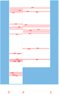
Figure 4: A storm in a coffee cup - non Newtonian chaos in a one dimensional step potential. The lines represent examples of non-Newtonian orbits in the potential (6). For illustration purposes different trajectories are shown at different energies, as well as different sections of same trajectories are shifted slightly up and down the energy axis, so that their parts are visible.

It should also be emphasized, that at every reflection or transmission (scattering) event, the particle completely looses its memory about the previous stage of its motion. Given the current position and the momentum of the particle, neither its previous evolution nor its state of motion after the next collision can be reconstructed. Hence, instead of the deterministic evolution we generated a fairly complicated stochastic dynamical process by considering a seemingly simple potential (6).

Obviously, there can be classical orbits of arbitrary length, and the bigger is the allowed length (or the period) of the trajectory, the larger are the numbers of nontrivial orbits that come into picture. Is there a way to enumerate all this variety the orbits? It turns out that the description of the general behavior of the orbits in this system can be conveniently formalized. Indeed, every orbit can be described by a two-letter code, which would simply tell us in what sequence the orbit swings through the left ($L$) or the right ($R$) sides of the well, as shown in (Fig. 4).

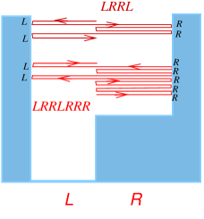
Figure 5: A couple of examples of a non-Newtonian orbits in the potential (6) marked by their R-L binary codes. Every left swing of the orbit contributes an “L” to its code and every right one contributes an “R”.

Periodic orbits are obviously represented by periodic sequences of symbols. Conversely, any periodic sequence of the symbols (for example, $RLRLRLRLRL...$ or just $(RL)$ for short), unambiguously describes a certain periodic orbit (note however, that two sequences which can be obtained from one another by a cyclical permutation of symbols, correspond to the same periodic orbit). If the orbit swings $n_{1}$ times in the left side of the well and $n_{2}$ in the right side, its action length is equal

$$S_{orb}=2n_{1}S_{1}+2n_{2}S_{2},$$ (13)

where $S_{1}=L_{1}k$ and $S_{2}=L_{2}\kappa$.

The number of the periodic orbits increases indefinitely. Their shapes (and correspondingly their $L-R$ binary codes) become more and more complicated, so the classical mechanics in the potential turns out to be surprisingly rich. In fact, the number of the geometrically different orbit shapes (or the number of the prime periodic orbits, the ones that never retrace themselves) that include up to $m$ scattering events grows exponentially as

$$N\approx\frac{e^{0.7m}}{m}.$$ (14)

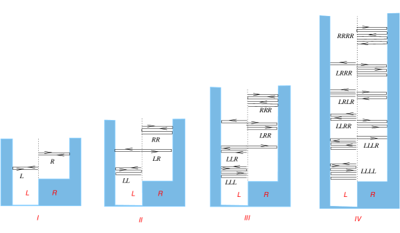
Figure 6: Exponential proliferation of the orbits in the potential (6). The orbits that undergo 1, 2, 3 and 4 scatterings marked by their R-L binary codes.

Such behavior closely resembles the periodic orbit proliferation scenario that takes place in classically nonintegrable chaotic systems. Hence a particle in the potential (6) can be viewed as a simple model of a classically chaotic system. This $L-R$ code representation of the orbits is a simple example of symbolic dynamics over a partition of the phase space Cvit ; Smale .

The difference between this and the simple back and forth motion in the square well potential is overwhelming, and provides a simple illustration to the difference between the dynamical behavior of the integrable and the nonintegrable systems, such as e.g. Hydrogen and Helium. The outburst of complexity that results after adding an extra potential step at the bottom of the potential (1) is similar to the situation with the Helium atom. An extra electron that is added to the two-body system of the nucleus and the electron in the Hydrogen atom totally destroys its integrability.

Of course the more complex is the orbit shape, the smaller is the probability that this particular orbit will be realized. This “complexity selection” can be easily understood from the point of view of the quantum mechanics, where the propagation of the particle is described by the normalized wave (2). It is clear that every reflection or transmission reduces its initial amplitude by the amount of the reflection or transmission coefficient. Hence, it is clear that if a certain prime periodic orbit $p$ (i.e. the one that can not be considered a repetition of a shorter orbit) reflects $\sigma(p)$ times from the either side of the potential barrier at $x=b$, and transmits $\tau(p)$ times through it, its initial amplitude will decrease

$$A_{p}=(-1)^{\chi(p)}r^{\sigma(p)}(1-r^{2})^{\tau(p)/2}$$ (15)

times Nova . Here the factor $(-1)^{\chi(p)}$ keeps track of the sign changes due to the wall reflections and the right reflections from the boundary. If the orbit $p$ is traced over itself $\nu$ times, then the corresponding amplitude will be $A_{p}^{\nu}$. So the quantity (15) is a certain quantum (and, since $r$ does not depend on $\hbar$, also classical) “weight” of the orbit.

V Classical Dynamics and Quantum Spectrum

In the case of the infinite square well potential the orbit bouncing back and forth between the walls of (1) completely exhausts all the classical dynamical possibilities of the particle in the infinite square well. This orbit also defines the quantum energy spectrum (4) of the particle via the relationship $S_{n}=\pi n$. This is analogous to the general quantization procedure of the so called integrable systems, i.e. the ones that have as many dynamically conserved quantities (e.g. angular momentum, etc.) as degrees of freedom Einstein ; Keller . These conserved quantities (the action integrals) $I_{i}$, $i=1,...,d$, are quantized according to

$$I_{i}=h(n_{i}+\mu_{i}),$$ (16)

where $n_{i}$s are natural numbers, $n_{i}=1,2,...$, and $\mu_{i}$ is a certain geometrical constant Maslov . The energy of these systems is a certain function of the $I_{i}$’s, $E=E(I_{1},...I_{N})$, and so the quantization rules (16) provide immediately the (semiclassical) energy spectrum. For example, for a particle moving in the infinite potential well (1), the magnitude of the momentum $|p|$, and hence the action, $I=2|p|L$, is conserved. It is then quantized as $|p|=\hbar\pi n/L$, and yields the quantum energy eigenvalues $E=(\hbar\pi n)^{2}/2mL^{2}$.

According to this scheme, the “quantum numbers” $n_{i}$ are naturally related to the classical integrals of motion $I_{i}$.

On the other hand, the classical behavior of the particle in the potential (6) is of manifestly nonintegrable type. The variety of possible dynamical orbits in the potential (6) is much richer than in (1), and we were able to describe all of them. What information is hidden in this variety of the orbits? Is it possible, after all, to use this knowledge to obtain the quantum energy spectrum? One should remember that most of these orbits appeared as some leftovers of purely quantum effects - the over-barrier reflections and under-barrier tunnelings. Do they carry through the complete quantum mechanical information about the particle?

As pointed out above, in the integrable systems there exists a convenient handle - the action integrals, which can be ascribed certain discrete values via the EBK semiclassical quantization procedure above Einstein ; Keller . What if the integrals do not exist? What is there in a nonintegrable system that can be used in order to quantize the system semiclassically?

The first answer to this question came in early 70s, when Gutzwiller Gutzwiller showed that a “handle” for semiclassical quantization of the systems without the sufficient number of the integrals of motion is provided by the so-called density of states - a functional that corresponds a $\delta$ -peak to every energy level $E_{n}$ of the quantum spectrum,

$$\rho(E)\equiv\sum_{n=1}^{\infty}\delta\left(E-E_{n}\right).$$ (17)

Gutzwiller provided a semiclassical expansion for $\rho(E)$ (the so-called Gutzwiller trace formula) in terms of the classical quantities related to the periodic orbits,

$$\rho(E)\approx\bar{\rho}(E)+\frac{1}{\pi}\mathop{\rm Re}\sum_{p}T_{p}\sum_{\nu=1}^{\infty}B_{p}^{\nu}\,e^{i\nu S_{p}(E)}.$$ (18)

Here $T_{p}$, $S_{p}$ and $B_{p}$ are correspondingly the period, the action and a certain weight factor (see below) of the prime periodic orbit $p$ (all classical quantities), and $\nu$ is the number of times the orbit $p$ repeats itself. The first term $\bar{\rho}(E)$ represents the non-oscillating part of the density of states.

The gist Gutzwiller’s trace formula is an (almost miraculous) interference effect, produced by the infinity of oscillating terms (one per each periodic orbit) in the sum (18). The statement made by (18) is that if the energy $E$ happens to coincide with a quantum energy level $E_{n}$, then all the terms in the sum (18) will interfere constructively and produce a peak, whereas if there are no quantum $E_{n}$’s there, they will interfere destructively and yield $0$.

This is a truly remarkable connection between the classical and the quantum properties of a system. After all, from a formal mathematical perspective, classical characteristics of a system should a priori describe only its $\hbar=0$ limit, whereas according to the trace formula one can use the classical properties of the system to extract the information about its quantum properties for $\hbar\neq 0$.

Gutzwiller’s formula can also be applied to the 1D system of a particle in the step potential (6). Moreover, it can be shown Nova that for the system (6) the expansion (18) is exact, although usually it provides only an approximate (with semiclassical accuracy) representation of $\rho(E)$. Another important characteristic of the spectrum is the “spectral staircase” $N(E)$,

$$N(E)\equiv\int_{0}^{E}\rho(E^{\prime})dE^{\prime}=\sum_{n}\Theta\left(E-E_{n}\right),$$ (19)

where $\Theta(x)$ is Heaviside’s theta function,

$$\Theta(x)=\cases{1,&if $x>0$,\cr 0&if $x<0$,\cr}$$ (20)

which gives the number of the energy levels on the interval between $0$ and $E$. $N(E)$ can also be expanded into a periodic orbit series,

$$N(E)=\bar{N}(E)+\frac{1}{\pi}\mathop{\rm Im}\sum_{p}\sum_{\nu=1}^{\infty}\frac{A_{p}^{\nu}}{\nu}\,e^{i\nu S_{p}(E)}.$$ (21)

What makes the expansion (21) particularly convenient for our use, is that the weight factors $A_{p}$ in it are explicitly given by (15). The first term of $N(E)$ (its non-oscillating part, also known as Weyl’s average) is given by

$$\bar{N}(E)=\frac{1}{\pi}S(E)-\gamma_{0},$$ (22)

where $S(E)$ is the action length (11) of the classically available region of the well, and $\gamma_{0}$ is a small correction term (almost a constant, see below).

The complexity of our task of describing the spectrum in (6) can already be appreciated from the expansions (18) and (21): every non-Newtonian orbit that exists in (6) explicitly contributes to these expansions.

In addition to the huge number of the periodic orbits, there are many other subtle dynamical effects that contribute to the complexity of the expansions (18) and (21). For instance, it was mentioned above that as the energy of the particle passes from above $V$ to a level below $V$, the particle becomes classically unable to penetrate into the right section of the well, $b<x<L$. However, there exists the possibility of quantum tunneling into the region $R$. This is manifested by the corresponding momentum becoming imaginary, $\kappa\rightarrow i\varkappa$. Hence, the contributions to the orbit actions (13) due to the “tunneling” through the step parts are also imaginary, $S_{orb}=2S_{1}n_{1}+i2n_{2}S_{2}$ (such orbits were called “ghost orbits” in Haake ).

That implies that as the energy of the particle changes, the physical characteristics of the orbits (and therefore of the expansion terms in (18)) may change (phenomenon known as the “phase space metamorphosis” PSM ). However, the formal structure of the Gutzwiller’s formula (at least in the case at hand) remains the same, and so the expansions (18) and (21) can be used, with due care, both for $E>V$ and for $E<V$.

VI Obtaining the spectrum

Since the right hand side of the expansion (18) can be obtained from considering the classical motion of the particle, the expansion (18) provides a clear connection between the dynamical characteristics of the system and its spectrum in quantum regime. The energy levels of the quantum system are obtained according to (18) as the poles (delta spikes) produced by the periodic orbit sum Gutzw ; Gutzwiller . It is important however, that by using this approach, one can not tell when these poles will appear prior to performing the summation of the periodic orbit series (18). Without having any extra information about the system, the only general strategy for obtaining $E_{n}$’s is to scan the energy axis by summing the series (18) for every value of $E$ to find out at what energies the sum produces a $\delta$-peak.

This illustrates the fact that $\rho(E)$ is a global characteristic of the spectrum. Both $\rho(E)$ and its expansion (18) describe the whole spectrum at once, rather than the specific individual energy levels, in contrast with the case of the integrable systems, where every action integral $I_{i}$ is quantized directly (16) and separately from the rest of the degrees of freedom.

Actually, it is possible to extract the information about the individual energy levels $E_{n}$ out of $\rho(k)$ without such tedious “energy axis scanning” - if only one knows (at least approximately) where to look. Indeed, if for instance we would happen to know that some energy level $E_{n}$ is the only level that lies between two points $\hat{E}_{n}^{+}$ and $\hat{E}_{n}^{-}$ (and hence $\rho(E)$ has only one $\delta$-peak between these points), then we could evaluate the integral

$$E_{n}=\int_{\hat{E}_{n}^{-}}^{\hat{E}_{n}^{+}}E\rho(E)dE,$$ (23)

and obtain the value of $E_{n}$. Since we know the expansion of $\rho(E)$ in terms of the periodic orbits (the right hand side of (18)), this integration (at least in principle) can be performed.

If our knowledge of a certain system would be so complete that we would be able to separate every energy level $E_{n}$ from its neighbors by two “separators” $\hat{E}_{n}^{+}$ and $\hat{E}_{n}^{-}$, $\hat{E}_{n}^{+}>E_{n}>\hat{E}_{n}^{-}$, then we could use (23) to obtain an exact numerical value of every energy level in the spectrum of our problem out of $\rho(E)$. Apparently, for the purpose of separating one level from another, it is enough to assume that $\hat{E}_{n-1}^{+}=\hat{E}_{n}^{-}$, so basically we are looking for a sequence of points $\hat{E}_{n}$ that interweaves the sequence of the energy levels and separates one energy level from another Opus ; Prima ; Sutra ; Stanza . In other words, in order to be able to obtain quantitatively any energy level $E_{n}$ out of $\rho(E)$, we need to establish a partition of the $E$-axis into the intervals $\left[\hat{E}_{n-1},\hat{E}_{n}\right]$, each one of which contains exactly one energy level.

Note, that even if that could be achieved, one would still have just an algorithmic recipe for evaluating $E_{n}$’s rather than a formula of the type $E_{n}=...$ . In order to get such a formula, we would need to find a global function $\hat{E}(n)$ that depends explicitly on $n$ and produces all the separating points in their natural sequence as a function of their index,

$$\hat{E}_{n}=\hat{E}(n).$$ (24)

Once such a functional dependence of the separators on their index is established, the integral (23) would turn the index $n$ into a quantum number and give us a complete solution to the spectral problem in the form $E_{n}=...$ .

The problem is that usually this is not an easy task. In order to establish a partition of the energy axis into the separating intervals $\left[\hat{E}_{n-1},\hat{E}_{n}\right]$ one needs to have some extra information about the behavior of the spectrum. Luckily, such information can be obtained for the particle in the potential (6).

VII Spectral equation

In order to get this information, let us examine closely the spectral equations (8) and (10). Since the quantity that we are after, the classical action $S(E)$ defined by (11) is in the arguments of the sines in the left hand sides of the equations (8) and (10), we can formally invert them to obtain

$$S=\pi\left(n-\frac{1}{2}\right)-\cases{(-1)^{n}\left(\arcsin\left(r\sin\left(S_{1}-S_{2}\right)+\frac{\pi}{2}\right)\right),&if $E>V$,\cr\arctan\left(\varkappa\left(1+e^{-2S_{2}}\right)/k\left(1-e^{-2S_{2}}\right)\right),&if $E<V$,\cr}$$ (25)

where $n=1,2,...\,$. This form of the spectral equation is particularly important for two reasons. First, we are getting an index $n$ which (one would assume) numbers the solutions $S_{n}$ - the discrete quantum values of action.

One can notice an interesting resemblance between the way the formulae (25) begin, $S=\pi\left(n-\frac{1}{2}\right)+...$, and the formula (16). One can speculate therefore that the first term, $\pi\left(n-\frac{1}{2}\right)$, expresses the regular part of the spectrum, and the second terms, which actually make the equation (25) transcendental, are introducing the irregularities into the spectrum, which are due to the classical non-integrability of the potential well (6).

This in fact turns out to be a very important observation. Is the spectrum defined by (25) more “regular” or “irregular”? Which one of these two terms contributes more to the solution, the regular $\pi\left(n-\frac{1}{2}\right)$ part or the irregular second term? Surprisingly, it turns out that in terms of the magnitudes the regular part wins. Indeed, it is well known that the inverse trigonometric functions are bounded, $-\frac{\pi}{2}\leq\arcsin(x),\arctan(x)\leq\frac{\pi}{2}$. On the other hand, when the index $n$ in the equation (25) changes by $1$ as we go from one level to another, the “regular term” increases by $\pi$, which is generically (that is almost always) more than what the arcsine or arctangent can provide.

Therefore, it is the regular first term $\pi\left(n-\frac{1}{2}\right)$ in (25) that contributes the most to the solution. If the step at the bottom of the well would disappear, so would the “transcendental” terms in (25), and a pure regular (periodic) spectrum (4) for $S$ would be recovered. Hence the second term in (25) can be regarded as the one responsible for the chaos induced spectral “fluctuations”.

The second important consequence of writing the equations (8) and (10) in the inverted form (25), is that it allows one to obtain the set of separating points discussed in the previous section, and hence to implement the solution to the spectral problem for the potential (6).

Indeed, since the irregular terms in (25) are different from $0$, the values $\hat{S}_{n}=\pi(n-1/2)$ themselves are never the solutions to (25). On the other hand, the difference between $\hat{S}_{n}$ and the roots $S_{n}$, which is due to the second term, is smaller than $\pi$, and as a result the roots $S_{n}$ of (25) will be locked inside of the intervals

$$\pi\left(n-\frac{1}{2}\right)<S_{n}<\pi\left(n+\frac{1}{2}\right).$$ (26)

Thus, the first discrete quantum action value will be locked between $\pi/2$ and $3\pi/2$, the second one between $3\pi/2$ and $5\pi/2$, and so on. In other words, we run immediately into the separating points for the quantum values of action,

$$\hat{S}_{n}=\pi(n-1/2),\ \ n=1,2,...\,,$$ (27)

or the action separators. These separators can be used to extract the energy separators $\hat{E}_{n}$ from $S(\hat{E}_{n})=\pi(n-1/2)$, which then can be used to obtain the energy spectrum via (23).

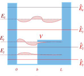
Figure 7: The energy separators $\hat{E}_{n}$ (their values on the energy scale are shown by solid lines) define the upper and the lower bounds for the quantum energy levels $E_{n}$, shown by the dashed lines.

Alternatively, rather than solving the equation $S(\hat{E}_{n})=\pi(n-1/2)$ for the $\hat{E}_{n}$’s in order to use them in the formula (23), one could introduce a “density of the action states”, $\rho(S)$, defined as $\rho(S)dS=\rho(E)dE$,

$$\rho(S)\equiv\sum_{n=1}^{\infty}\delta\left(S-S_{n}\right)\frac{dE}{dS},$$ (28)

to obtain the actual quantum levels of action first and then to extract the quantum energy levels from them. This would completely parallel the $\rho(E)$ approach outlined in the previous section. A simple change of variables will produce the periodic orbit expansion for $\rho(S)$. Hence it is possible, in accordance with the ideas outlined above, to obtain the discrete quantum action values $S_{n}$ via

$$S_{n}=\int_{\pi(n-1/2)}^{\pi(n+1/2)}S\rho(S)dS=S\,N(S)\Big{|}_{\pi(n-1/2)}^{\pi(n+1/2)}-\int_{\pi(n-1/2)}^{\pi(n+1/2)}N(S)\,dS,$$ (29)

where we used the identity

$$\rho(S)=\frac{dN(S)}{dS}.$$ (30)

Using the relationship $N(\hat{S}_{n})=n$ (there are exactly $n$ roots $s_{n}$ below the $n$th separator) and the expansion (21), we get

$$S_{n}=2\pi n-\frac{\pi}{2}-\int_{\pi(n-1/2)}^{\pi(n+1/2)}\bar{N}(S)dS-\frac{1}{\pi}\mathop{\rm Im}\sum_{p,\nu}\int_{\pi(n-1/2)}^{\pi(n+1/2)}\frac{A_{p}^{\nu}}{\nu}e^{i\nu S_{p}}dS,$$ (31)

where the weight factors $A_{p}$ are given by (15).

Note, that (4) is exactly the first term of the expansion (31). Hence the oscillatory terms in (31), with their amplitudes proportional to the non-Newtonian reflection amplitudes, are indeed due to the “nonintegrability” of (6).

Since all of the quantities on the right-hand side of (31) are known, this formula provides an explicit representation of the discrete quantum values of the action functional in terms of the geometric and dynamical characteristics of the potential (6). Formula (31) allows the computation of the action corresponding to every quantum level individually, explicitly and exactly in terms of the classical parameters, indexed by its “quantum number” $n$.

It should be mentioned however, that the quantum number $n$ in (4) and in (31) have rather different origins. Formula (31) does not have such a direct geometrical interpretation as (4). While in (4) the number $n$ is the number of waves that fit on the trajectory, in the case of the step potential (6) $n$ is the index of the cell (26) that contains the corresponding action value $S_{n}$.

So once again, we arrive at defining the quantum energy spectrum via a discrete set of allowed values of the action functional, $S_{n}=S(E_{n})$. This relationship (which is yet to be presented explicitly) can be viewed as a direct generalization of (4).

Of course, for using the periodic orbit expansions in practice, one needs to know how to truncate the series (18) or (31) to obtain finite order approximations to $S_{n}$. Since usually the periodic orbit series are not absolutely convergent, the order in which the expansion terms are incorporated into the sum (31) is important. It turns out Opus ; Prima ; Sutra ; Stanza , that the correct way to obtain $m$th approximation to the exact value of $S_{n}$ is to include into the sum (31) all the trajectories that reach the point $x=b$ $m$ times or less.

VIII Overview and an example

Let us summarize the steps for obtaining the $m$th correction to $S_{n}$ using the semiclassical periodic orbit expansion technique.

1. Write down all the $m$-letter sequences (words) $w_{m}$. For example, there are 2 words, $(L)$ and $(R)$, for $m=1$, 4 words $(LL)$, $(LR)$, $(RL)$ and $(RR)$ for $m=2$, 8 words $(LLL)$, $(LLR)$, $(LRL)$, $(RLL)$, $(RLR)$, $(RRL)$, $(LRR)$ and $(RRR)$ for $m=3$ and so on. (To do the same thing geometrically - draw all possible periodic orbits similar to the ones shown in Fig. 5 that include exactly $m$ transmissions and reflections).

2. Find which $w$’s are cyclic permutations of one another - all these sequences represent the same orbit, so pick one and discard its replicas. From the above examples, both $m=1$ orbits will remain, for $m=2$ we may keep $(LL)$, $(LR)$ and $(RR)$, for $m=3$ we keep $(LLL)$, $(LLR)$, $(RLR)$ and $(RRR)$. (Geometrically: find out which loops are representing the same sequence of left and right swings. Pick one and discard its replicas).

3. Count the number $n_{L}$ of $L$’s and $n_{R}$ of $R$’s in $w$ and find the action $S_{w}$ of the orbit $w$ according to

   $$S_{w}=2n_{R}S_{1}+2n_{L}S_{2}.$$ (32)

   Remember that if $E<V$ then $S_{2}=i\sqrt{V-E}L_{2}$.

4. Assuming that the first symbol in $w$ cyclically follows the last one, find out which of the remaining sequences $w$ are prime sequences and which ones are repetitions of a shorter code. Find the repetition number $\nu_{w}$ for each orbit (use $\nu_{w}=1$ if the orbit is prime). For example, for $m=2$ the orbit $\nu_{LR}=1$, $\nu_{RR}=\nu_{LL}=2$, and for $m=3$ $\nu_{LLL}=\nu_{RRR}=3$, $\nu_{LLR}=\nu_{RLR}=1$. (Geometrically, find out how many times each orbit traverses over itself).

5. Scan each word $w_{m}$ (again, the first symbol of $w$ follows the last one) and write down the weight $A_{w}$ according to the substitutions

   $$LR\rightarrow t,\ \ RL\rightarrow t,\ \ LL\rightarrow r,\ \ RR\rightarrow-r,$$ (33)

   plus each wall reflection contributes a sign change. For example, for $m=1$, $A_{L}=-r$, $A_{R}=r$, for $m=2$ $A_{LR}=t^{2}$, $A_{RR}=A_{LL}=r^{2}$, and for $m=3$ we have $A_{LLL}=-r^{3}$, $A_{RRR}=r^{3}$, $A_{LLR}=-rt^{2}$, $A_{RLR}=rt^{2}$. (Geometrically: assign a factor $t$ to every transmission, a factor $-1$ to every wall reflection, a factor $r$ to every left side reflection and a factor $-r$ to every right side reflection).

6. For every orbit, find out the corresponding term in the expansion (31),

   $$\int_{\pi(n-1/2)}^{\pi(n+1/2)}\frac{A_{w}}{\nu_{w}}e^{iS_{w}(S)}dS,$$ (34)

   and integrate.

If all the words up the length $m$ are considered, the result will produce $m$th approximation to the exact discrete sequence of actions.

All the non-Newtonian orbits described in the previous sections contribute to the expansion of each eigenvalue $S_{n}$. One can now appreciate the complexity of solving analytically the equations (8) and (10) compared to solving the simple equation (3), by comparing the complexities of the corresponding classical dynamics.

VIII.1 An example

As an example, let us compute the first three approximations to a a few momentum eigenvalues, using the orbits that include up to 3 scattering events, outlined in the summary and shown in Fig. 6.

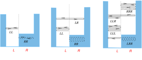
Figure 8: The orbits required for evaluating the first three periodic orbit expansion approximations to the $S_{n}$. Since the evaluation of the low levels which correspond to the energy $E<V$ will require ghost orbits, a few ghost orbits are also illustrated. The tunneling parts of the ghost orbits are shown with dashed lines.

We have according to (31) that the first three corrections will be:

$$S_{n} = 2\pi n-\frac{\pi}{2}-\int_{\pi(n-1/2)}^{\pi(n+1/2)}\bar{N}(S)dS$$ (35)

$$- \mathop{\rm Im}\int_{\pi(n-1/2)}^{\pi(n+1/2)}\left(re^{i2S_{1}k}-e^{i2S_{2}k}r\right)dS$$ (36)

$$- \mathop{\rm Im}\int_{\pi(n-1/2)}^{\pi(n+1/2)}\left(\frac{1}{2}r^{2}e^{4iS_{1}}+t^{2}e^{i2S_{1}+i2S_{2}}+\frac{1}{2}e^{4iS_{2}}r^{2}\right)dS$$ (37)

$$- \mathop{\rm Im}\int_{\pi(n-1/2)}^{\pi(n+1/2)}\left(\frac{1}{3}r^{3}e^{6iS_{1}}+t^{2}re^{i\left(2S_{2}+4S_{1}\right)}-t^{2}\allowbreak re^{i\left(2S_{1}+4S_{2}\right)}-\frac{1}{3}r^{3}e^{6iS_{2}}\right)dS.$$ (38)

In order to use the formula (38), one needs to specify the parameters of the potential well (6). In particular, it is a specific value of $V$ that determines at what energy the periodic orbits will acquire tunneling parts. For simplicity, let us consider the case of symmetrical well, when $L_{1}=L_{2}=1$. Then the action $S$ defined by (11) will be

$$S(E)=\cases{k+\kappa,&if $E>V$,\cr k&if $E<V$,\cr}$$ (39)

in terms of which

$$\cases{r=\frac{V}{S^{2}},\ \ t^{2}=\left(1-\frac{V^{2}}{S^{4}}\right),&if $E>V$,\cr r=e^{2i\pi\gamma_{0}},\ \ \gamma_{0}=\frac{1}{\pi}\arctan\frac{\sqrt{V-S^{2}}}{S},\ \ t^{2}=\left(1-e^{2i\pi\gamma_{0}}\right)&if $E<V$.\cr}$$ (40)

The phase $\gamma_{0}$ (which also appears in the Weyl’s average (22)) is $\gamma_{0}=1/2$ for $E>V$.

Next, let us pick a certain value for the potential step hight, say $V=25$. This will set the $E_{crit}=25$ and $k_{crit}=5$ to be the “critical values” of energy and the momentum - that is if we will be looking for an energy level below $E=V=25$, then the tunneling effects (ghost orbits, the restructuring of the periodic orbit sum (18)) have to be taken into account. Correspondingly, the critical value for the action will be $S_{crit}=k_{crit}L_{1}=5$, and so one should use different parts of formulae (39) to extract the $E_{n}$ or $k_{n}$ out of $S_{n}$, depending on whether a particular $s_{n}$ is smaller or greater than $5$.

After the height of the potential step has been chosen, certain general statements about the behavior of the quantum $S_{n}$ levels can be made. For the specific case $V=25$, the first and the second separators, $\hat{S}_{1}=\frac{\pi}{2}$ and $\hat{S}_{2}=\frac{3\pi}{2}$, will be smaller than $S_{crit}$, and so the level contained between them will correspond to the energy $E_{1}<V$. The third action separator is bigger than $k_{crit}$, $\hat{S}_{3}=5\pi/2>5$, so we will be in a better position to judge about the location of the second level $\hat{S}_{2}<S_{2}<\hat{S}_{3}$ after computing the corrections (38). All the other levels $S_{n}$, for $n>2$, have energies higher than $V$.

So let us find the discrete quantum action values $S_{1}$, $S_{2}$ and (for example) $S_{17}$, and the corresponding quantum momentum eigenvalues, $k_{1}$, $k_{2}$ and $k_{17}$. Using the expressions (38), (39), (40) and integrating from $\pi/2$ to $3\pi/2$, from $3\pi/2$ to $5\pi/2$ and from $33\pi/2$ to $35\pi/2$ (using some numerical integration software is highly recommended) we find the values shown in Table 1.

root	$m=0$	$m=0$	$m=2$	$m=3$		exact
$s_{1}$	2.4354	2.6198	2.6173	2.605		2.5958787201295728
$s_{2}$	6.1601	5.5789	5.2366	5.1434		4.9455316914381690
$s_{17}$	53.4071	53.405	53.404	53.406		53.403119615030526

Table 1: The results of the periodic orbit expansion approximations to the exact values of $s_{n}$. The first $m=0$ column gives the Weyl’s $s_{n}^{(m=0)}$ estimate for the roots of the spectral equation, and the following columns show the corrections to it due to the $m=1$, $m=2$ and $m=3$ code length orbits. Note that the third periodic orbit expansion approximation to $s_{2}$ comes out higher than the critical value, $s_{2}^{(m=3)}>s_{crit}=5$, whereas the actual root $s_{2}$ is smaller than $s_{crit}$. Hence more periodic orbit expansion terms are needed to capture the correct qualitative behavior of $s_{2}$.

Note that in the second case the integration in (38) should be split in two parts,

$$\int_{3\pi/2}^{5\pi/2}N(S)dS=\int_{3\pi/2}^{5}N^{(E<S)}(S)dS+\int_{5}^{5\pi/2}N^{(E>V)}(S)dS,$$ (41)

in order to follow the changes in the structure of the expansion terms described by (39) and (40). Note also that the column to column changes are more significant for the second root - this indicates that the “spectral fluctuations” for this root are high due to the orbit metamorphosis that takes place at $E=V$, inside of the integration interval $\hat{E}_{n-1}<E_{n}<\hat{E}_{n}$. This also indicates that more periodic orbit expansion terms are needed to get the more precise position of $s_{2}$ with respect to $V$.

After the allowed values $S_{n}$ for the action are found, the quantum levels of the momentum can be obtained by inverting the relationship (39),

$$k=\cases{\frac{s^{2}-V}{2s},&if $s_{n}<V$,\cr s&if $s_{n}<V$.\cr}$$ (42)

According to (1) one has from (42):

$$k_{1}=2.605,\ \ k_{2}=5.0020,\ \ k_{17}=26.4689.$$ (43)

(44)

This demonstrates how the periodic orbit expansion quantization rule (31) gives the explicit solution to our spectral problem.

IX A simplification - scaling potential

It is possible to simplify significantly the result by assuming that the hight of the potential step $V$ also grows (scales) with energy, $V=\lambda\,E$. This assumption is not as artificial as it may seem. Scaling (not necessarily in the $V=\lambda\,E$ form) is a common phenomenon that occurs in a variety of familiar physical systems PSM ; Tom , such as, e.g. the Hydrogen atom in a uniform magnetic field (also a nonintegrable system). Basically, the scaling eliminates the geometrical restructuring of the trajectories - i.e. in our case the transitions from classically allowed to “ghost” to orbits.

As soon as a certain value of the scaling coefficient $\lambda$ has been chosen, the orbits will either always hover above the potential step ($\lambda<1$) or sit below it ($\lambda>1$). The assumption $V=\lambda\,E$ also implies that the reflection coefficient $r_{sc}$ (and therefore the weight factors (15)) do not depend on energy,

$$r_{sc}=\frac{1-\beta}{1+\beta},$$ (45)

where $\beta=\sqrt{1-\lambda}$. In addition, the action lengths of the two parts of the potential (6) become simply proportional to $k$, $S_{1}=L_{1}k$ and $S_{2}=L_{2}\beta k$. The spectral equation for $\lambda<1$ is now

$$\sin(\Omega_{0}k)=r_{sc}\sin(\omega k)$$ (46)

where $\Omega_{0}=L_{1}+\beta L_{2}$ and $\omega=L_{1}-\beta L_{2}$ are constant frequencies, $\Omega_{0}>\omega$, and the roots of (46) are separated from one another by a periodic sequence of separators

$$\hat{k}_{n}=\frac{\pi}{\Omega_{0}}\left(n+\frac{1}{2}\right).$$ (47)

For a given $\lambda$, the coefficients $r_{sc}$, $\Omega_{0}$, $\omega$ and the separators (47) do not depend on energy anymore. The spectral equation (46) doesn’t change its functional form, and the tunneling (ghost) trajectories never appear in the system. This clearly illustrates the idea of the “structural freezing” of the dynamics due to the scaling.

With so many characteristics of the system becoming constant, the evaluation of the $k_{n}$ greatly simplifies and the integration in (31) can be carried out explicitly Opus ; Prima ; Sutra ; Stanza .

Let us assume that energy scales above the potential step, $\lambda<1$. The exact eigenvalues of the momentum in this case are

$$k_{n}=\frac{\pi}{\Omega_{0}}n-\frac{2}{\pi}\sum_{p}\frac{1}{S_{p}^{0}}\sum_{\nu=1}^{\infty}\frac{A_{p}^{\nu}}{\nu^{2}}\sin\left(\frac{\nu\omega_{p}}{2}\right)\,\sin\left(\nu\omega_{p}n\right),$$ (48)

where $S_{p}^{0}=S_{p}/k$, $\omega_{p}=\pi S_{p}^{0}/S_{0}$, and the weight factors $A_{p}$ are given by (15) in which $r=r_{sc}$. This expression clarifies the overall structure of the periodic orbit expansions for $k_{n}$.

X Discussion

We have studied an elementary example of a classically nonintegrable (quantum stochastic) system in the potential (6). Despite the simplicity of the setup, the classical dynamics of the particle in the potential (6) turns out to be extremely complicated, and this complexity is manifested in its spectral properties in quantum regime. Surprisingly, in studying this most elementary example, one runs into essentially all the dynamical and physical effects (integrability versus nonintegrability, the exponential proliferation of the periodic orbits in the nonintegrable case, periodic orbit expansions, the use of symbolic dynamics, phase space metamorphosis, tunneling, ray splitting, etc.) that appear in semiclassical analysis of more realistic physical systems. Usually these phenomena are investigated via a rather involved mathematical apparatus, whereas in our example they naturally come into play and can be analyzed by elementary means. Due to its illustrative simplicity, this and similar Anima ; Saga ; Fabula systems can be thought of as the “Harmonic oscillators” of quantum chaos. On the other hand, this problem is rich enough to illustrate the essence of the difficulties associated with the semiclassical quantization of chaotic dynamical systems, such as Helium atom.

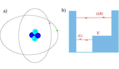
Figure 9: The familiar schematic picture of the Helium atom (Fig. 7a), which was also used as the physical model in 1920s, is analogous to using only Newtonian trajectories in the potential (6), shown in Fig. 7b. This scheme completely ignores the actual classical dynamical complexity. Compare the Fig. 7(b) to Fig. 3 and Fig. 5.

As mentioned above, the early attempts to quantize the Helium atom failed because the qualitative difference in the dynamical complexity between Hydrogen and Helium were overlooked. The attempts to quantize a chaotic system within the framework of Bohr-Sommerfeld or EBK quantization theory using only a few integrable-like trajectories can be compared to considering just the two “naive” (Newtonian) classical trajectories in the potential (6), $(L)$ for $E<V$ and $(LR)$ for $E>V$. From the structure of the exact result (31) it is clear that such consideration would produce only very approximate results, far from the real complexity of the problem.

Formula (31) represents the “modification” of the EBK quantization condition (4) mentioned in the Van Vleck citation above, for the simple case of the potential (6), in an explicit and self-contained form. It would be natural to expect that obtaining the semiclassical spectrum in the form $E_{n}=...$ for more complicated systems such as Helium atom should be a much more difficult task. However, this result creates an interesting precedent that may indicate new directions in the semiclassical quantization theory and related fields.

- (1) M. C. Gutzwiller, Chaos in Classical and Quantum Mechanics (Springer, New York, 1990).
- (2) P. Cvitanović, R. Artuso, R. Mainieri, G. Tanner and G. Vattay, Classical and Quantum Chaos, www.nbi.dk/ChaosBook/, Niels Bohr Institute (Copenhagen 2001)
- (3) K. G. Kay, Phys. Rev. Lett. 83 n. 25 p. 5190 (1999); K. G. Kay, Phys. Rev. A, 63, 042110 (2001) and 65, 032101 (2002)
- (4) N. Bohr, On the application of the quantum theory to atomic structure Cambridge [Eng.] The University press, (1924).
- (5) J. H. van Vleck, Philos. Mag. 44 p. 842 (1922).
- (6) M. Born, Vorlesungen über Atommechanik Springer, Berlin, (1925) translated in Mechanics of the Atom, Ungar, New York, (1927).
- (7) A. M. Lyapunov, General motion stability problem Doctoral dissertation (1890), in Russian; Recherches dans la theorie des corps celestes (1903).
- (8) H. Poincaré, Les méthodes nouvelles de la mécanique céleste, translated in New methods of celestial mechanics, AIP, Woodbury, NY, (1992).
- (9) J. Hadamard, OEuvres de Jacques Hadamard Paris, Éditions du Centre national de la recherche scientifique (1968).
- (10) G. D. Birkhoff, Dynamical systems AMS, New York, (1927), Proc. Natl. Acad. Sci. USA 17, 656 (1931).
- (11) A. Einstein, Zum Quantensatz von Sommerfeld und Epstein Deutsche Physikalische Gesellschaft, Verhandlungen 19, 82-92 (1917).
- (12) D. Wintgen, K. Richter and G. Tanner, CHAOS 2,(1), p.19, (1992)
- (13) D. J. Griffith, Introduction to Quantum Mechanics, Prentice Hall, Inc. (1995).
- (14) S. Flügge, Practical Quantum Mechanics (Berlin, Springer, 1999).
- (15) A. Messiah, Quantum Mechanics, (North-Holland, New York, 1961).
- (16) L. D. Landau and E. M. Lifshitz, Quantum Mechanics (Pergamon Press, New York, 1977).
- (17) R. E. Prange, E. Ott, T. M. Antonsen, B. Georgeot, and R. Blümel, Phys. Rev. E 53, 207 (1996).
- (18) R. Blümel, T. M. Antonsen, Jr., B. Georgeot, E. Ott, and R. E. Prange, Phys. Rev. Lett. 76, 2476 (1996); Phys. Rev. E 53, 3284 (1996).
- (19) V. P. Maslov and M. V. Fedoriuk, Kvaziklassicheskoe priblizhenie dlia uravnenii kvantovoi mekhaniki, Nauka, Moscow (1976), translated in Semiclassical Approximation in Quantum Mechanics, D. Reidel Pub. Co., Dordrecht, Holland (1981).
- (20) M. C. Gutzwiller, J. Math. Phys., 8 p. 1979 (1967); 10 p. 1004 (1969); 11 p. 1791 (1970); 12 343 (1971); 14 p. 139 (1973).
- (21) M. Kuś, F. Haake, Prebifurcation Periodic Ghost Orbits in Semiclassical Quantization, Phys. Rev. Lett, 71, 2167, (1993).
- (22) Y. C. Lai, C. Grebogi, R. Blümel, and M. Ding, Phys. Rev. A 45, 8284 (1992).
- (23) M. Keeler and T. J. Morgan, Phys. Rev. Lett. 80, 5726 (1998).
- (24) S. Smale, Differentiable Dynamical Systems, Bull AMS 73, p. 747.
- (25) J. B. Keller Ann. Phys. (N.Y.) 4, 180 (1958).
- (26) Y. Dabaghian, R. V. Jensen and R. Blümel, Phys. Rev. E 63, 066201 (2001).
- (27) Y. Dabaghian, R. V. Jensen and R. Blümel, Pis’ma v ZhETF 74, 258 (2001), JETP Letters 74 (4) 235 (2001).
- (28) R. Blümel, Y. Dabaghian and R. V. Jensen, Phys. Rev. Lett. 88, 044101 (2002).
- (29) R. Blümel, Y. Dabaghian and R. V. Jensen, Phys. Rev. E 65, 046222 (2002)
- (30) Y. Dabaghian, R. V. Jensen and R. Blümel, ZhETF, 121, N 6 (2002).
- (31) Y. Dabaghian and Blümel, JETP Letters, Vol 77, No 9, pp 530-533 (2003)
- (32) Yu. Dabaghian and R. Bl mel, Explicit, Phys. Rev. E 68, 055201(R) (2003).
- (33) Y. Dabaghian, Blümel, submitted to PRE (2004).