Analytical results for entanglement in the five-qubit anisotropic Heisenberg model

Abstract

We solve the eigenvalue problem of the five-qubit anisotropic Heisenberg model, without use of Bethe’s Ansatz, and give analytical results for entanglement and mixedness of two nearest-neighbor qubits. The entanglement takes its maximum at $\Delta=1$ ($\Delta>1$) for the case of zero (finite) temperature with $\Delta$ being the anisotropic parameter. In contrast, the mixedness takes its minimum at $\Delta=1$ ($\Delta>1$) for the case of zero (finite) temperature.

Recently, the study of entanglement properties of many-body systems has received much attention M_Nielsen -QPT_GVidal . To obtain analytical results for entanglement, one may consider the case of infinite lattice or a small lattice with a few qubits. It is hard to get some analytical results between these two extreme cases.

It was well-known that the anisotropic Heisenberg model can be solved formally by Bethe’s Ansatz method Bethe ; Yang for arbitrary number of qubits $N$, however, we have to solve a set of transcendental equations. For $N\leq 7$, the isotropic Heisenberg Hamiltonian can be analytically solved Kouzoudis ; Schnack . Here, we give the analytical results of the eigenvalues of the anisotropic Heisenberg model with $N=5$, without use of Bethe’s Ansatz, from which the analytical expressions for entanglement and mixedness of two nearest-neighbor qubits are readily obtained.

It is interesting to see that the entanglement properties of a pair of nearest-neighbor qubits at a finite temperature is completely determined by the partition function. The entanglement, quantified by the concurrence Conc , relates to the partition function $Z$ via Glaser ; Gu ; WangPaolo

$$C=\max\left(0,\Big{|}\frac{U}{N}-\frac{1}{2}-\frac{\Delta G_{zz}}{2}\Big{|}-\frac{G_{zz}}{2}-\frac{1}{2}\right)$$ (1)

with

$$U=-\frac{\partial\ln Z}{\partial\beta}$$ (2)

being the internal energy, and

$$G_{zz}=\text{Tr}[\exp(-\beta H)\sigma_{iz}\sigma_{i+1z}]/Z=-\frac{2}{N\beta}\frac{\partial\ln Z}{\partial\Delta}$$ (3)

being the correlation function. Here, $\beta=1/T$ and the Boltzmann’s constant $k=1$. Thus, once we know the eigenenergies versus the temperature and the anisotropic parameter, we can completely determine the entanglement.

There exists another concept, the mixedness of a state, is central in quantum information theory Jaeger . For instance, Bose and Vedral have shown that entangled states become useless for quantum teleportation on exceeding a certain degree of mixedness Bose . Mixedness is also related to quantum entanglement. We will study both the entanglement and mixedness properties.

Eigenvalue problem. The anisotropic Heisenberg Hamiltonian is given by

$$H= \frac{J}{2}\sum_{i=1}^{N}\left(1+\sigma_{ix}\sigma_{i+1x}+\sigma_{iy}\sigma_{i+1y}+\Delta\sigma_{iz}\sigma_{i+1z}\right)$$

$$= J\sum_{i=1}^{N}\left(S_{i,i+1}+\frac{\Delta-1}{2}\sigma_{iz}\sigma_{i+1z}\right),$$ (4)

where $S_{j,j+1}=$$\frac{1}{2}\left(1+\vec{\sigma}_{i}\cdot\vec{\sigma}_{i+1}\right)$ is the swap operator between qubit $i$ and $j$, $\vec{\sigma}_{i}=(\sigma_{ix},\sigma_{iy},\sigma_{iz})$ is the vector of Pauli matrices, and $J$ is the exchange constant. We have assumed the periodic boundary condition, i.e., $N+1\equiv 1$. In the following discussions, we also assume $J=1$ (antiferromagnetic case) and $\Delta\geq 0$.

Since we impose the periodic boundary condition, the Hamiltonian is translational invariant, i.e., $[H,T]=0$, where $T$ is the cyclic right shift operator defined as

$$T|m_{1},\cdots,m_{N-1},m_{N}\rangle=|m_{N},m_{1},\cdots,m_{N-1}\rangle.$$ (5)

The translational invariant symmetry can be used to reduce the Hamiltonian matrix to smaller submatrices by a factor of $N$ Lin .

Now we focus our attention to five-qubit settings, and solve the eigenvalue problem of the anisotropic Heisenberg model. Since $[H,J_{z}]=0$, the whole 32-dimentional Hilbert space can be divided into invariant subspaces spanned by vectors with a fixed number of reversed spins. Then, the largest subspace is 10-dimensional with 2 or 3 reversed spins. Here, $J_{z}=\sum_{i=1}^{5}\sigma_{iz}/2$. Due to the symmetry $[H,\Sigma_{x}]=0$, it is sufficient to solve the eigenvalue problems in the subspaces with $r$ reversed spins, where $r\in\{0,1,2\}$ and $\Sigma_{x}=\sigma_{x}\otimes\sigma_{x}\otimes\sigma_{x}\otimes\sigma_{x}\otimes\sigma_{x}.$ By using the translational invariance, we can further reduce the Hamiltonian matrix to $2\times 2$ submatrices, and the eigenvalue problem can be readily solved.

The subspace with $r=0$ only contains one vector $|00000\rangle$, which is the eigenvector with eigenvalue

$$E_{0}=5[1+(\Delta-1)/2].$$ (6)

The subspace with $r=1$ is spanned by five basis vectors $\{T^{n}|10000\rangle,n\in\{0,1,2,3,4\}\}$. Considering the translational invariance of the Hamiltonian, we choose another basis given by

$$|\varphi_{k}\rangle=\sum_{n=0}^{4}\omega^{n}_{k}T^{n}|10000\rangle,$$ (7)

where $\omega_{k}=e^{\frac{i2k\pi}{5}},k\in\{1,2,3,4,5\}$. It can be checked that states $|\varphi_{k}\rangle$ are eigenstates of $T$ with eigenvalues $\omega_{k}^{-1}$, and are also eigenstates of Hamiltonian $H$ with eigenvalues given by

$$E_{1,k}=3+\frac{\Delta-1}{2}+2\cos(2k\pi/5).$$ (8)

For the case of $r=2$, we choose the following basis for 10-dimensional subspace

$$|\psi_{k}\rangle=\sum_{n=0}^{4}\omega_{k}^{n}T^{n}|11000\rangle,$$

$$|\phi_{k}\rangle=\sum_{n=0}^{4}\omega_{k}^{n}T^{n}|10100\rangle.$$ (9)

States $|\psi_{k}\rangle$ and $|\phi_{k}\rangle$ span an invariant $2\times 2$ subspace under the action of Hamiltonian $H$. In this subspace, the Hamiltonian can be written as

$$H_{k}=\left(\begin{array}[]{ll}3+\frac{\Delta-1}{2}&1+\omega_{k}^{-1}\\ 1+\omega_{k}&1-\frac{3(\Delta-1)}{2}+\omega_{k}^{2}+\omega_{k}^{-2}\end{array}\right).$$ (10)

Then, from the above equation, the eigenvalues are obtained as

$$E_{2,k\pm}= \frac{5-\Delta+2\cos(4k\pi/5)}{2}$$

$$\pm \sqrt{[\Delta-\cos(4k\pi/5)]^{2}+2[1+\cos(2k\pi/5)]}.$$ (11)

Thus, all eigenvalues are obtained for the five-spin anisotropic Heisenberg models. We see that eigenstates are at least two-fold degenerate due to the symmetry $[H,\Sigma_{x}]=0$. Although the eigenstates can be easily obtained, they are not given explicitly here as the knowledge of eigenvalues is sufficient for discussions of entanglement and mixedness properties.

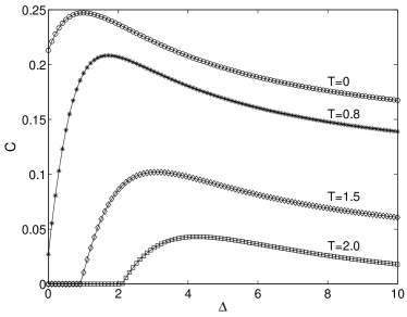
Figure 1: The concurrence versus $\Delta$ for different temperatures.

Entanglement and mixedness. From Eqs. (1)–(3), the concurrence is determined by the partition function and its derivative with respect to the anisotropic parameter $\Delta$. As we have obtained all eigenvalues of five-spin Hamiltonian $H$, from Eqs. (6)-(8), it follows that

$$Z=2\left[e^{-\beta E_{0}}+\sum_{k=1}^{5}\left(e^{-\beta E_{1,k}}+e^{-\beta E_{2,k+}}+e^{-\beta E_{2,k-}}\right)\right].$$ (12)

Substituting the above equation into Eqs. (2) and (3) yields

$$U= \frac{2}{Z}\Big{[}E_{0}e^{-\beta E_{0}}+\sum_{k=1}^{5}(E_{1,k}e^{-\beta E_{1,k}}$$

$$+E_{2,k+}e^{-\beta E_{2,k+}}+E_{2,k-}e^{-\beta E_{2,k-}})\big{]},$$ (13)

and

$$G_{zz}= \frac{2}{5Z}\Big{[}\frac{5}{2}e^{-\beta E_{0}}+\sum_{k=1}^{5}\big{(}\frac{1}{2}e^{-\beta E_{1,k}}$$

$$+ \frac{\partial E_{2,k+}}{\partial\Delta}e^{-\beta E_{2,k+}}+\frac{\partial E_{2,k-}}{\partial\Delta}e^{-\beta E_{2,k-}}\big{)}\Big{]}.$$ (14)

with

$$\frac{\partial E_{2,k\pm}}{\partial\Delta}=-\frac{1}{2}\pm\frac{\Delta-\cos(4k\pi/5)}{\sqrt{[\Delta-\cos(4k\pi/5)]^{2}+2[1+\cos(2k\pi/5)]}}.$$ (15)

Then, the analytical expressions of the internal engery $U$ and the correlation function $G_{zz}$ are obtained, and thus, according to Eq. (1), we get the analytical expression of the concurrence for the thermal state.

At zero temperature, the system is in the ground state, and for this case, Eq. (1) reduces to

$$C=\max\left(0,\big{|}\frac{E_{gs}}{N}-\frac{1}{2}-\frac{\Delta}{N}\frac{\partial E_{gs}}{\partial\Delta}\big{|}-\frac{1}{N}\frac{\partial E_{gs}}{\partial\Delta}-\frac{1}{2}\right),$$ (16)

where $E_{gs}$ denotes the ground-state energy and $N=5$. In the derivation of the above equation, we have used the relation

$$G_{zz}=\frac{2}{N}\langle\frac{\partial H}{\partial\Delta}\rangle=\frac{2}{N}\frac{\partial E_{gs}}{\partial\Delta},$$ (17)

which is valid for the ground state. For our five-qubit model, $E_{gs}=E_{2,1-}$ and the derivative of $E_{gs}$ with respect to $\Delta$ is given by Eq. (15). Thus, the analytical expression for the entanglement of ground state is obtained. If $\frac{E_{gs}}{N}-\frac{1}{2}-\frac{\Delta}{N}\frac{\partial E_{gs}}{\partial\Delta}\leq 0$, then Eq. (16) reduces to

$$C=-\frac{E_{gs}}{N}+\frac{\Delta-1}{N}\frac{\partial E_{gs}}{\partial\Delta},$$ (18)

where we have ignored the max function. Taking derivative with respect to $\Delta$ on both sides of the above equation leads to

$$\frac{\partial C}{\partial\Delta}=\frac{\Delta-1}{N}\frac{\partial^{2}E_{gs}}{\partial^{2}\Delta}.$$ (19)

Then, it is direct to check from the above equation and the ground state energy $E_{2,1-}$ (11) that the derivative is zero when $\Delta=1$. Thus, the concurrence takes its extreme value at the point of $\Delta=1$ for the ground state.

From the analytical results for the concurrence, we numerically plot the concurrence versus the anisotropic parameter for different temperatures in Fig. 1. We observe that the concurrence takes its maximum when $\Delta=1$. This point correspond to the critical point of metal-insulation transition Gu . However, for finite temperature, the concurrence reaches its maximum when $\Delta>1$. For finite temperatures (for instance, $T=2.0$), we find a threshold value of the anisotropic parameter $\Delta_{\text{th}}$, before which there is no pairwise entanglement. The threshold value increase as temperature increases.

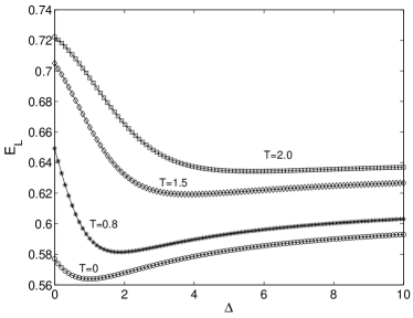
Figure 2: The linear entropy versus $\Delta$ for different temperatures.

Next, we study mixedness properties of the thermal state and ground state. The mixedness of a state $\varrho$ can be quantified by the linear entropy given by $E_{L}=1-\text{Tr}(\varrho^{2}).$ Then, for arbitrary number of qubits, the linear entropy of the state of two nearest qubits is given by

$$E_{L}(T)=1-\frac{1}{4}\left[2\Big{(}\frac{U}{N}-\frac{1}{2}-\frac{\Delta G_{zz}}{2}\Big{)}^{2}+{G_{zz}}^{2}+{1}\right]$$ (20)

for the thermal state, and

$$E_{L}(T=0)= 1-\frac{1}{4}\Big{[}2\Big{(}\frac{E_{gs}}{N}-\frac{1}{2}-\frac{\Delta}{N}\frac{\partial E_{gs}}{\partial\Delta}\Big{)}^{2}$$

$$+\frac{4}{N^{2}}\Big{(}\frac{\partial E_{gs}}{\partial\Delta}\Big{)}^{2}+{1}\Big{]}$$ (21)

for the ground state, respectively. We see that the mixedness of the thermal state is also completely determined by the partition function, and the mixedness of the ground state is determined by the ground-state energy and its first-order derivative with respect to the anisotropic parameter. Thus, the analytical expressions of the linear entropy are obtained.

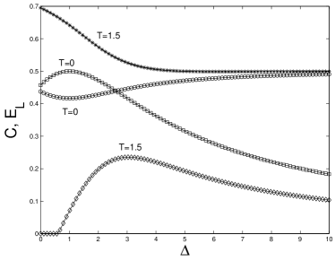
Figure 3: The concurrence (square and diamond lines) and linear entropy (circle and star lines) versus $\Delta$ for different temperatures in the four-qubit model.

In Fig. 2, we numerically calculated the linear entropy versus $\Delta$ for different temperatures. In contrast to the entanglement, the mixedness of the ground state displays a minimum when $\Delta=1$. For the case of finite temperatures, the mixedness takes its minimum when $\Delta>1$. For lower temperatures (for instance, $T\leq 0.2$), numerical results show that the maximum of the concurrence occurs nearly at the same value of $\Delta$ as the minimum of the mixedness. It seems that the more the pairwise entanglement, the less the mixedness. However, for higher temperatures, the maximum of the concurrence and the minimum of the mixedness do not occur at the same $\Delta$. For instance, when $T=1.5$, the concurrence takes its maximum at $\Delta=3.1037$, and the mixedness takes its minimum at $\Delta=3.8525$. This signifies that it is not always true that the more the pairwise entanglement and the less the mixedness.

For the case of four qubits, the anisotropic Heisenberg model is also exactly solvable using the same method as above. Here, we make a comparison of the four-qubit and five-qubit cases. The exact ground-state energy and its derivative with respect to $\Delta$ are given by

$$E_{gs}=2-\Delta-\sqrt{\Delta^{2}+8},\;\frac{\partial E_{gs}}{\partial\Delta}=-1-\frac{\Delta}{\sqrt{\Delta^{2}+8}}.$$ (22)

Substituting the above equation into Eqs. (16) and (21), we obtain the ground-state concurrence and linear entropy as

$$C(T=0)= \frac{\Delta+8}{4\sqrt{\Delta^{2}+8}}-\frac{1}{4},$$

$$E_{L}(T=0)= \frac{11}{16}-\frac{\Delta}{8\sqrt{\Delta^{2}+8}}-\frac{\Delta^{2}+32}{16(\Delta^{2}+8)}.$$ (23)

From the above analytical expressions, it is straightforward to check that the concurrence takes its maximum and the linear entropy takes its minimum at the point of $\Delta=1$, which is exactly the same feature as that in the five-qubit model. For finite temperatures, in Fig. 3, we give numerical calculations of the concurrence and the linear entropy. We see that they displays similar behaviours as those in the five-qubit model. For instance, for $T>0$, the maximum pairwise entanglement and the minimum mixedness occur at $\Delta>1$.

Conclusion. In conclusion, we have obtained the analytical results for the entanglement and mixedness in the five-qubit anisotropic Heisenberg model. The exact eigenspectrum is obtained, and entanglement and mixedness properties can be completely determined by the eigenvalues of the system, irrespective of the eigenstates. The method adopted here can be applied to the anisotropic Heisenberg model with more than five qubits (for instance, 6 or 7 qubits). However, the analytical expressions for eigenvalues, entanglement, and mixedness are expected to be more complicated.

We have made numerical calculations, and show that the entanglement takes its maximum at $\Delta=1$ ($\Delta>1$) for the case of zero (finite) temperature. In contrast, the mixedness takes its minimum at $\Delta=1$ ($\Delta>1$) for the case of zero (finite) temperature. From our analysis, we conjecture that it is a general feature that at zero temperature the entanglement takes its maximum and the mixedness takes its minimum when $\Delta=1$ for any number of qubits. This conjecture is supported by our analytical results for four and five qubits, and by numerical results for the number of qubits being as large as 1280 Gu . The Heisenberg chains not only displays rich entanglement features, but also have useful applications such as the quantum state transfer M_Sub . Experimentally, it was found that entanglement is crucial to describing magnetic behaviors in a quantum spin system Exp . So, the study of entanglement and mixedness properties in the Heisenberg models will strength our understanding of other quantum features of magnetic systems.

- (1) M. A. Nielsen, Ph. D thesis, University of Mexico, 1998, quant-ph/0011036;
- (2) M. C. Arnesen, S. Bose, and V. Vedral, Phys. Rev. Lett. 87, 017901 (2001).
- (3) D. Gunlycke, V. M. Kendon, V. Vedral, and S. Bose, Phys. Rev. A64, 042302 (2001).
- (4) X. Wang, Phys. Rev. A 64, 012313 (2001); Phys. Lett. A 281, 101 (2001).
- (5) X. Wang, H. Fu, and A. I. Solomon, J. Phys. A: Math. Gen. 34, 11307(2001); X. Wang and K. Mølmer, Eur. Phys. J. D 18, 385(2002).
- (6) G. L. Kamta and A. F. Starace, Phys. Rev. Lett. 88, 107901 (2002).
- (7) K. M. O’Connor and W. K. Wootters, Phys. Rev. A63, 0520302 (2001).
- (8) D. A. Meyer and N. R. Wallach, quant-ph/0108104.
- (9) T. J. Osborne and M. A. Nielsen, Phys. Rev. A66, 032110 (2002).
- (10) A. Osterloh, L. Amico, G. Falci and R. Fazio, Nature 416, 608 (2002).
- (11) Y. Sun, Y. G. Chen, and H. Chen, Phys. Rev. A 68, 044301 (2003).
- (12) L. F. Santos, Phys. Rev. A67, 062306 (2003).
- (13) Y. Yeo, Phys. Rev. A66, 062312 (2002).
- (14) D. V. Khveshchenko, Phys. Rev. B68, 193307 (2003).
- (15) L. Zhou, H. S. Song, Y. Q. Guo, and C. Li, Phys. Rev. A68, 024301 (2003).
- (16) G. K. Brennen, S. S. Bullock, quant-ph/0406064.
- (17) G. Tóth and J. I. Cirac, quant-ph/0406061.
- (18) F. Verstraete, M. Popp, and J. I. Cirac, Phys. Rev. Lett. 92, 027901 (2004).
- (19) F. Verstraete, M. A. Martin-Delgado, J. I. Cirac, Phys. Rev. Lett. 92, 087201 (2004).
- (20) J. Vidal, G. Palacios, and R. Mosseri, Phys. Rev. A 69, 022107 (2004).
- (21) N. Lambert, C. Emary, and T. Brandes, Phys. Rev. Lett. 92, 073602 (2004).
- (22) G. Vidal, J. I. Latorre, E. Rico, and A. Kitaev Phys. Rev. Lett. 90, 227902 (2003)
- (23) H. A. Bethe, Z. Phys. 71, 205 (1931).
- (24) C. N. Yang and C. P. Yang, Phys. Rev. 150, 321 (1966).
- (25) D. Kouzoudis, J. Magn. Magn. Mater. 173, 259 (1997); ibid 189, 366 (1998).
- (26) K. Bärwinkel, H.-J. Schmidt, and J. Schnack, J. Magn. Magn. Mater. 220, 227 (2000).
- (27) W. K. Wootters, Phys. Rev. Lett. 80, 2245 (1998).
- (28) U. Glaser, H. Büttner, and H. Fehske, Phys. Rev. A68, 032318 (2003).
- (29) S. J. Gu, H. Q. Lin, and Y. Q. Li, Phys. Rev. A68, 042330 (2003).
- (30) X. Wang and P. Zanardi, Phys. Lett. A 301, 1 (2002); X. Wang, Phys. Rev. A 66, 044305 (2002).
- (31) G. Jaeger, A. V. Sergienko, B. E. A. Saleh, and M. C. Teich, Phys. Rev. A68, 022318 (2003).
- (32) S. Bose and V. Vedral, Phys. Rev. A61, 040101 (2000).
- (33) H. Q. Lin, Phys. Rev. B42, 6561 (1990).
- (34) S. Bose, Phys. Rev. Lett. 91, 207901 (2003); V. Subrahmanyam, Phys. Rev. A69, 034304 (2004); M. Christandl, N. Datta, A. Ekert, and A. J. Landahl, Phys. Rev. Lett. 92, 187902 (2004); Y. Li, T. Shi, Z. Song, and C. P. Sun, quant-ph/0406159; M. B. Plenio and F. L Semião, quant-ph/0407034.
- (35) S. Ghose, T. F. Rosenbaum, G. Aeppli, and S. N. Coppersmith, Nature (London) 425, 48 (2003).