Incoherent coincidence imaging and its applicability in X-ray diffraction

Abstract

Entangled-photon coincidence imaging is a method to nonlocally image an object by transmitting a pair of entangled photons through the object and a reference optical system respectively. The image of the object can be extracted from the coincidence rate of these two photons. From a classical perspective, the image is proportional to the fourth-order correlation function of the wave field. Using classical statistical optics, we study a particular aspect of coincidence imaging with incoherent sources. As an application, we give a proposal to realize lensless Fourier-transform imaging, and discuss its applicability in X-ray diffraction.

Optical imaging techniques using classic light sources have been the primary tools for scientific research and industrial applications. In recent years, there has been an increasing interest in the field of quantum imaging, in which nonclassical states of light are used as light sources epjdsyh ; rev ; jetp ; init ; entangle ; theory ; retrodic ; macro ; qlith ; qoct ; qholo ; amp . Special attentions are focused on entangled-photon coincidence imaging epjdsyh ; rev ; jetp ; init ; entangle ; theory ; retrodic ; macro .

The role of entanglement in coincidence imaging leads to some debates now. The authors in Ref entangle stated that only quantum entangled sources can be used to realize coincidence imaging, and using classical light sources can not produce the image of the object. However, using classically correlated beams, the experiment performed in classic also produced a coincidence image. Moreover, in a recent preprint bsincoh , it was shown using quantum theory that an object can be imaged via coincidence imaging with split incoherent thermal radiation. In this letter, we give a completely classical description of coincidence imaging and obtain a relationship between the intensity correlation in the detectors and the source. Especially, with a proper choice of the imaging geometry, we find it is possible to realize a kind of lensless Fourier-transform imaging by using an incoherent light source, which may be applicable for X-ray diffraction.

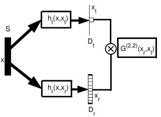
Figure 1: A setup of entangled-photon coincidence imaging. The source $S$ emits pairs of entangled photons. One of the photons transmits through the test system $h_{t}(x,x_{t})$ which contains an unknown object, and the other photon transmits through a known reference system $h_{r}(x,x_{r})$. Two detectors $D_{t}$ and $D_{r}$ record the intensity distribution. The coincidence rate $G^{(2,2)}(x_{r},x_{t})$ is measured to give a image of the object.

An example of the setup of a coincidence imaging system is shown in Fig (1) theory ; retrodic . If the source $S$ produces pairs of entangled photons, the produced photons are transmitted through a known (reference) optical system and an unknown optical system (test) which contains the object to be imaged. These two optical systems are characterized by their impulse response function $h_{r}(x,x_{r})$ and $h_{t}(x,x_{t})$ respectively. Two detectors $D_{1}$ and $D_{2}$ record the intensity distribution of the test and reference photons. The coincidence rate of photon pairs at these two detectors ($G^{(2,2)}(x_{r},x_{t})$) is proportional to the fourth-order correlation function of the optical fields,

$$G^{(2,2)}(x_{r},x_{t})=<I(x_{r})I(x_{t})>,$$ (1)

where $<...>$ means the ensemble average. In entangled-photon imaging, the object can be extracted from the marginal coincidence rate ($I^{(2)}(x_{r})=\int\!dx_{t}\,G^{(2,2)}(x_{r},x_{t})$) or the conditional coincidence rate ($I_{0}^{(2)}(x_{r})=G^{(2,2)}(x_{r},0)$) theory . Although the reference photons do not pass through the object, the object contained in the test system can be imaged at the reference detector. Such a nonlocal imaging technique may be useful for secure information transfer.

Now, suppose the light source $S$ is a classical light source, we use classically statistical optics to describe the coincidence imaging process. In the framework of fluctuating optical fields goodman , the forth-order correlation function $G^{(2,2)}(x_{r},x_{t})$ relates to the optical fields in the reference and test detectors by

$$G^{(2,2)}(x_{r},x_{t})=<E_{r}^{*}(x_{r})E_{t}^{*}(x_{t})E_{r}(x_{r})E_{t}(x_{t})>,$$ (2)

where $E_{r}(x_{r})$ is the optical field in the reference detector and $E_{t}(x_{t})$ is the optical field in the test detector. For simplicity, we assume the source is quasi-monochromatic with a mean wavelength $\lambda$. Only one transverse dimension ($x$) is considered though the generalization to two transverse dimension is straightforward.

If the optical field in the source is represented by $E(x)$, the propagation of $E(x)$ through two different optical systems leads to

$$E_{k}(x_{k})=\int\!dx\,E(x)h_{k}(x,x_{k}),$$ (3)

where $k=r,t$. Note that $h_{r}$, $h_{t}$ are deterministic functions, by substituting Eq. (3) into Eq. (2), we have

$$G^{(2,2)}(x_{r},x_{t})$$ (4)

$$= \int\!dx_{1}dx_{1}^{\prime}dx_{2}dx_{2}^{\prime}\,G^{(2,2)}(x_{1},x_{1}^{\prime},x_{2},x_{2}^{\prime})$$

$$\times h_{r}(x_{1},x_{r})h_{r}^{*}(x_{1}^{\prime},x_{r})h_{t}(x_{2},x_{t})h_{t}^{*}(x_{2}^{\prime},x_{t}).$$

where

$$G^{(2,2)}(x_{1},x_{1}^{\prime},x_{2},x_{2}^{\prime})=<E^{*}(x_{1}^{\prime})E^{*}(x_{2}^{\prime})E(x_{1})E(x_{2})>$$ (5)

is the fourth-order correlation function of the optical fields at the light source.

Eq. (4) establishes the relation between the coincidence rate at the detectors and the correlation at the source. We need to know the properties of the light source to go further. In many cases, the field fluctuations of a classical light source can be modeled by a complex circular Gaussian random process with zero mean goodman , then

$$G^{(2,2)}(x_{1},x_{1}^{\prime},x_{2},x_{2}^{\prime}) = G^{(1,1)}(x_{1},x_{1}^{\prime})G^{(1,1)}(x_{2},x_{2}^{\prime})+$$ (6)

$$G^{(1,1)}(x_{1},x_{2}^{\prime})G^{(1,1)}(x_{2},x_{1}^{\prime}),$$

where $G^{(1,1)}(x_{i},x_{j})$ is the second-order correlation function of the fluctuating source field, represented by $G^{(1,1)}(x_{i},x_{j})=<E^{*}(x_{i})E(x_{j})>$, and satisfies $G^{(1,1)}(x_{i},x_{j})=\left[G^{(1,1)}(x_{j},x_{i})\right]^{*}$.

Substituting Eq. (6) into Eq. (4), we get

$$G^{(2,2)}(x_{r},x_{t}) = \left(\int\!dx_{1}dx_{1}^{\prime}\,G^{(1,1)}(x_{1},x_{1}^{\prime})h_{r}(x_{1},x_{r})h_{r}^{*}(x_{1}^{\prime},x_{r})\right)\times\left(\int\!dx_{2}dx_{2}^{\prime}\,G^{(1,1)}(x_{2},x_{2}^{\prime})h_{t}(x_{2},x_{t})h_{t}^{*}(x_{2}^{\prime},x_{t})\right)$$ (7)

$$+\left(\int\!dx_{1}dx_{2}^{\prime}\,G^{(1,1)}(x_{1},x_{2}^{\prime})h_{r}(x_{1},x_{r})h_{t}^{*}(x_{2}^{\prime},x_{t})\right)\times\left(\int\!dx_{2}dx_{1}^{\prime}\,G^{(1,1)}(x_{2},x_{1}^{\prime})h_{t}(x_{2},x_{t})h_{r}^{*}(x_{1}^{\prime},x_{r})\right)$$

$$= <I_{r}(x_{r})><I_{t}(x_{t})>+\left|\int\!dx_{1}dx_{2}^{\prime}\,G^{(1,1)}(x_{1},x_{2}^{\prime})h_{r}(x_{1},x_{r})h_{t}^{*}(x_{2}^{\prime},x_{t})\right|^{2},$$

The first term in the right side of Eq. (7) is the multiplication of the intensity distribution at the reference and test detectors, and cannot be used to realize the coincidence imaging entangle ; theory . However, if $G^{(1,1)}(x_{1},x_{2})$ is not factorable, the second term in the right side of Eq. (7) has the similar form as in the entangled-photon coincidence imaging, apart from the presence of a phase conjugated $h_{t}^{*}$ instead of $h_{t}$. Since a second-order correlation function of a classical light source is factorable only when the source is fully coherent, we can perform the coincidence imaging using partially coherent or incoherent light sources.

Let us introduce the intensity fluctuations in the two detectors

$$\Delta I_{k}(x_{k})=I_{k}(x_{k})-<I_{k}(x_{k})>,$$ (8)

in which $k=r,t$. The correlation between the intensity fluctuations at the reference and test detectors is

$$<\Delta I_{r}(x_{r})\Delta I_{t}(x_{t})>$$ (9)

$$= \left|\int\!dx_{1}dx_{2}^{\prime}\,G^{(1,1)}(x_{1},x_{2}^{\prime})h_{r}(x_{1},x_{r})h_{t}^{*}(x_{2}^{\prime},x_{t})\right|^{2}.$$

This correlation function is experimentally measurable. A similar result has been derived in Ref. bsincoh , but quantum theory is used in the derivation.

Based on Eq. (9), we propose a scheme to realize lensless Fourier-transform imaging by selecting proper $h_{r}$ and $h_{t}$.

Suppose the light source is fully spatially incoherent, then

$$G^{(1,1)}(x_{1},x_{2})=I(x_{1})\delta(x_{1}-x_{2}),$$ (10)

where $I(x)$ is the intensity distribution of the source and $\delta(x)$ is the Dirac delta function.

Further, the reference system contains nothing but free-space propagation from $S$ to $D_{r}$. Under the paraxial approximation, the impulse response function of the reference system is

$$h_{r}(x,x_{r})=\frac{e^{-ikd_{r}}}{i\lambda d_{r}}\exp\left\{\frac{-i\pi}{\lambda d_{r}}(x-x_{r})^{2}\right\}.$$ (11)

where $\lambda$ is the source wavelength and $k=2\pi/\lambda$ is the wave number, $d_{r}$ is the distance between $S$ and $D_{r}$.

The test system comprises an object at a distance $d_{1}$ from $S$ and a distance $d_{2}$ from $D_{t}$. The wave emitted from the source propagates freely to the object characterized by the transmittance $t(x^{\prime})$, then after transmission, it propagates freely to the test detector. The impulse response function of such a test system is

$$h_{t}(x,x_{t})=\int\!dx^{\prime}\,\frac{e^{-ikd_{1}}}{i\lambda d_{1}}\exp\left\{\frac{-i\pi}{\lambda d_{1}}(x-x^{\prime})^{2}\right\}t(x^{\prime})\frac{e^{-ikd_{2}}}{i\lambda d_{2}}\exp\left\{\frac{-i\pi}{\lambda d_{2}}(x_{t}-x^{\prime})^{2}\right\}.$$ (12)

Substituting Eqs. (10,11,12) into Eq. (9), after some calculations, we have

$$<\Delta I_{r}(x_{r})\Delta I_{t}(x_{t})>$$ (13)

$$= \left|\int\!dx^{\prime}dx\,I(x)\frac{e^{ikd_{r}}}{-i\lambda d_{r}}\exp\left\{\frac{i\pi}{\lambda d_{r}}(x-x_{r})^{2}\right\}\frac{e^{-ikd_{1}}}{i\lambda d_{1}}\exp\left\{\frac{-i\pi}{\lambda d_{1}}(x-x^{\prime})^{2}\right\}t(x^{\prime})\frac{e^{-ikd_{2}}}{i\lambda d_{2}}\exp\left\{\frac{-i\pi}{\lambda d_{2}}(x_{t}-x^{\prime})^{2}\right\}\right|^{2}.$$

If the source is large enough and the intensity distribution is uniform, we can regard $I(x)=I_{0}$, then Eq. (13) becomes

$$<\Delta I_{r}(x_{r})\Delta I_{t}(x_{t})>=\left|\int\!dx^{\prime}\,I_{0}\frac{e^{-ik(d_{1}-d_{r})}}{i\lambda(d_{1}-d_{r})}\exp\left\{\frac{-i\pi}{\lambda(d_{1}-d_{r})}(x_{r}-x^{\prime})^{2}\right\}t(x^{\prime})\frac{e^{-ikd_{2}}}{i\lambda d_{2}}\exp\left\{\frac{-i\pi}{\lambda d_{2}}(x_{t}-x^{\prime})^{2}\right\}\right|^{2}.$$ (14)

Selecting $d_{1}$, $d_{2}$ and $d_{r}$ to satisfy $d_{1}-d_{r}=-d_{2}$, the quadratic terms of $x^{\prime}$ can be canceled, Eq. (14) has the form

$$<\Delta I_{r}(x_{r})\Delta I_{t}(x_{t})> = \left|\int\!dx^{\prime}\,\frac{I_{0}}{\lambda^{2}d_{2}^{2}}\exp\left\{\frac{-i\pi}{\lambda d_{2}}(x_{t}^{2}-x_{r}^{2})\right\}t(x^{\prime})\exp\left\{\frac{i2\pi(x_{t}-x_{r})x^{\prime}}{\lambda d_{2}}\right\}\right|^{2}$$ (15)

$$= \frac{I_{0}^{2}}{\lambda^{4}d_{2}^{4}}\left|T\left(\frac{2\pi(x_{t}-x_{r})}{\lambda d_{2}}\right)\right|^{2},$$

where $T(q)$ is the Fourier transformation of $t(x^{\prime})$. So the correlation function between the intensity fluctuations at the reference and test detectors is the Fourier transformation of the transmittance of the object. We note that the appearance of $h^{*}_{t}$ rather than $h_{t}$ in Eq. (7) allows this particular result to be obtained without the use of a lens anywhere in the system.

If we measure the conditional correlation function of the intensity fluctuations by using a point-like test detector located at $x_{t}=0$,

$$\Delta I_{0}^{(2)}(x_{r})=<\Delta I_{r}(x_{r})\Delta I_{t}(0)>,$$ (16)

it will generate a image recorded in the reference detector but contains the information of the object. Equations (15) and (16) then yield

$$\Delta I_{0}^{(2)}(x_{r})=\frac{I_{0}^{2}}{\lambda^{4}d_{2}^{4}}\left|T\left(\frac{-2\pi x_{r}}{\lambda d_{2}}\right)\right|^{2}.$$ (17)

So we found that, under the conditions of a large, uniform, fully incoherent light source, without any optical instruments (such as lens) in the reference and test systems, using a point-like detector $D_{t}$ and an array of pixel detectors $D_{r}$, such a coincidence imaging system realizes the function of Fourier-transform imaging.

Due to the success of the oversampling approach, coherent X-ray diffraction imaging has attracted much attention recently [16-18]. However, several factors still limit the imaging quality. Because it is very difficult to fabricate optical components (such as lenses) that function in the X-ray regime, free-space propagation is used to obtain the diffraction pattern. Also, it is well known that currently used X-ray sources are generally incoherent. To achieve the spatial coherence needed to form high-quality diffraction patterns, such X-ray sources must be small and far from the object [19]. These requirements decrease the illumination efficiency and necessitate the use of high brightness sources such as synchrotron sources.

The lensless Fourier-transform imaging proposal given in this letter can overcome these difficulties. In fact, the image obtained in Eq. (17) is exactly the diffraction intensity pattern of the object. Since there is no requirement on the fully coherence, any kind of X-ray source can be used to realize X-ray diffraction imaging. As our method is insensitive to phase fluctuations of the source, the signal-to-noise ratio will be better than that achieved in direct diffraction imaging with an incoherent (or perhaps even partially coherent) source. So the incoherent coincidence imaging technique is applicable for X-ray diffraction.

Finally, we would like to discuss the effects of the time response of the detectors on our new imaging scheme. Generally, the intensity correlation $<I_{r}(x_{r})I_{t}(x_{t})>$ is not exactly measurable due to the finite time response of the detectors. Instead, we can only measure

$$<I^{\prime}_{r}(x_{r},t)I^{\prime}_{t}(x_{t},t+\tau)>$$ (18)

$$= \eta\int_{t-T_{R}/2}^{t+T_{R}/2}\int_{t+\tau-T_{R}/2}^{t+\tau+T_{R}/2}<I_{r}(x_{r},t^{\prime})I_{t}(x_{t},t^{\prime\prime})>$$

$$\times dt^{\prime}dt^{\prime\prime}.$$

where we write down the time dependence explicitly. In Eq. (18), $\eta$ is a coefficient and $T_{R}$ is the average time response of the detectors. Since in our imaging scheme, the free space propagation distance in $h_{r}$ and $h_{t}$ are equal, the time delay $\tau\approx 0$. In X-ray range, $T_{R}$ is much larger than the coherent time of the fluctuated fields, so the integration of Eq. (18) will be proportional to the equal-time intensity correlation $<I_{r}(x_{r})I_{t}(x_{t})>$ tai . Actually, in recent synchrotron radiation experiments, spatial intensity correlation have been measured by using slowly response detectors SRcorr . The key point is that, since only spatial intensity correlation is concerned in our imaging scheme, using slowly response detectors will screen the temporal fluctuation and measure the spatial intensity correlation only.

In conclusion, we have shown that a classically incoherent light source can be used to realize coincidence imaging based on the measurement of the correlation between the intensity fluctuations. Our treatments are fully classical and do not use quantum theory. As an application, a scheme to realize lensless Fourier-transform imaging is described, which may be very useful in X-ray diffraction imaging. These results will be generalized to three dimensional and the effects of source distribution or other imperfections will be considered in future works.

The authors are grateful to the reviewers for their helpful comments. This work was partly supported by the National Natural Science Foundation of China under Grant 69978023.

References

• (1) Y. Shih, Eur. Phys. J. D 22 485 (2003).
• (2) L.A. Lugiato, A. Gatti, and E. Brambilla, J. Opt. B 4 S176 (2002).
• (3) A.V.Β Belinsky and D.N.Β Klyshko, Sov.Β Phys JETP 78, 259 (1994).
• (4) D.V. Strekalov, A.V. Sergienko, D.N. Klyshko and Y.H. Shih, Phys. Rev. Lett. 74, 3600 (1995); T.B. Pittman, Y.H. Shih, D.V. Strekalov and A.V. Sergienko, Phys. Rev. A 52, R3429 (1995); P.H.S. Ribeiro, S.Padua, J.C.Machado da Silva and G.A. Barbosa, Phys. Rev. A 49 4176 (1994).
• (5) A.F. Abouraddy, B.E.A. Saleh, A.V. Sergienko, and M.C. Teich Phys.Β Rev.Β Lett.Β 87, 123602 (2001);
• (6) A.F. Abouraddy, B.E.A. Saleh, A.V. Sergienko, and M.C. Teich J. Opt. Soc. Am. B 19, 1174 (2002).
• (7) E.-K. Tan, J. Jeffers, S.M. Barnett, and D.T. Pegg, Eur. Phys. J. D 22 495 (2003).
• (8) A.Gatti, E. Brambilla,L.A. Lugiato, Phys.Rev.Lett. 90, 133603-1 (2003)
• (9) A.N. Boto, P. Kok, D.S. Abrams, S.L. Braunstein, C.P. Williams, and J.P. Dowling, Phys. Rev. Lett. 85 2733 (2000); M. D’Angelo, M.V. Cwckhova, and Y.H. Shih, Phys. Rev. Lett. 87 013602 (2001).
• (10) M.B. Nasr, B.E.A. Saleh, A.V. Sergienko, and M.C. Teich, Phys. Rev. Lett. 91 083601 (2003); A.F. Abouraddy, M.B. Nasr, B.E.A. Saleh, A.V. Sergienko, and M.C. Teich, Phys. Rev. A 65 053817 (2002).
• (11) A.F. Abouraddy, B.E.A. Saleh, A.V. Sergienko, and M.C. Teich, Opt. Express 9 498 (2001).
• (12) S-K. Choi, M. Vasilyev, and P. Kumar, Phys. Rev. Lett. 83 1938 (1999).
• (13) R.S. Bennink, S.J. Bentley and R.W. Boyd, Phys. Rev. Lett 89 113601 (2002).
• (14) A. Gatti, E. Brambilla, M. Bache and L.A. Lugiato, e-print quanth-ph/0307187.
• (15) J.W. Goodman, Statistical optics (Wiley, New York, 1985).
• (16) J. Miao, D. Sayre, and H.N. Chapman, J. Opt. Soc. Am. A 15 1662 (1998).
• (17) J. Miao, P. Charalambous, J. Kirz, and D. Sayre, Nature (London) 400 342 (1999).
• (18) I.K. Robinson, I.A. Vartanyants, G.J. Williams, M.A. Pfeifer, J.A. Pitney, Phys. Rev. Lett. 87 195505 (2001); J. Miao, T. Ishikawa, B. Johnson, E.H. Anderson, B. Lai, and K.O. Hodgson, Phys. Rev. Lett. 89 088303 (2002); G.J. Williams, M.A. Pfeifer, I.A. Vartanyants, and I.K. Robinson, Phys. Rev. Lett. 90 175501 (2003).
• (19) I.A. Vartanyants and I.K. Robinson, J. Phys.: Condens. Matter 13 10593 (2001).
• (20) R.Z. Tai, Y. Takayama, N. Takaya, T. Miyahara, S. Yamamoto, H. Sugiyama, J. Urakawa, H. Hayano, and M. Ando, Rev. Sci. Instrum. 71 1256 (2000).
• (21) R.Z. Tai, Y. Takayama, N. Takaya, T. Miyahara, S. Yamamoto, H. Sugiyama, J. Urakawa, H. Hayano, and M. Ando, Phys. Rev. A 60 3262 (1999); M. Yabashi, K. Tamasaku, and T. Ishikawa, Phys. Rev. Lett. 87 140801 (2001); K. Tamasaku, M. Yabashi, and T. Ishikawa. Phys. Rev. Lett. 88 044801 (2002).