Atomic diffraction by a thin phase grating

Abstract

We present a semiclassical perturbation method for the description of atomic diffraction by a weakly modulated potential. It proceeds in a way similar to the treatment of light diffraction by a thin phase grating, and consists in calculating the atomic wavefunction by means of action integrals along the classical trajectories of the atoms in the absence of the modulated part of the potential. The capabilities and the validity condition of the method are illustrated on the well-known case of atomic diffraction by a Gaussian standing wave. We prove that in this situation the perturbation method is equivalent to the Raman-Nath approximation, and we point out that the usually-considered Raman-Nath validity condition can lead to inaccuracies in the evaluation of the phases of the diffraction amplitudes. The method is also applied to the case of an evanescent wave reflection grating, and an analytical expression for the diffraction pattern at any incidence angle is obtained for the first time. Finally, the application of the method to other situations is briefly discussed.

1 Introduction.

The diffraction of atomic de Broglie waves by standing wave light fields [1-4] or mechanical microstructures [5] has recently received considerable interest because of its potential application as an atomic beam splitter, one of the key components for the development of atom optics and interferometry [6]. Among the different realizations of atom diffraction gratings proposed to date, the near-resonant Kapitza-Dirac effect [7] (the diffraction of atom from a standing laser field) has led by far to the most theoretical work [8]. Widespread interest in this effect arose because the phenomenon is the quantum mechanical analog of diffraction of light waves by a matter grating and also because it is conceptually one of the simplest examples of stimulated momentum transfer between atoms and light. The theoretical description of such a transmission diffraction is greatly simplified in the Raman-Nath regime of diffraction [1] where the change in kinetic energy of the atoms due to diffraction is neglected compared to the atom-field coupling. The problem then reduces to one dimension and the diffraction grating acts as a thin phase grating (the interaction between the atoms and the stationary laser wave only affects the phase of the atomic wavefunction). In contrast, the theoretical treatment of atomic diffraction by an evanescent wave reflection grating [3, 4] is known to lead to several unusual problems, which are related to the fact that the motion perpendicular to the diffraction grating can no longer be eliminated in a constant motion approximation. Indeed, the slowing down and eventually the reversal of the atomic motion is intrinsically associated with the reflection grating, and the problem remains necessarily two-dimensional. As a consequence, only a few attempts [3, 4] have been made to describe this diffraction process, and to our knowledge, no theoretical treatment provides a clear physical picture of atomic diffraction in the limit of small saturation of the atomic transition (a regime of great interest in atom optics experiments).

We present in this paper a semiclassical perturbation method which permits the treatment of atomic diffraction by a weakly modulated potential. The method applies both for transmission and reflection gratings, and proceeds in a way similar to the treatment of light diffraction by a thin phase grating. It is based on the evaluation of the atomic wavefunction by means of action integrals along the classical trajectories of the atoms calculated in the absence of the modulated part of the potential. In order to illustrate the capabilities and the limits of the perturbation method, we first consider the well-known near-resonant Kapitza-Dirac effect for which we prove the equivalence between our method and the Raman-Nath approximation. Furthermore, we show that the commonly-accepted validity condition of the latter actually leads to inaccuracies in the phases of the diffraction amplitudes. The case of atomic diffraction by a weakly modulated evanescent wave grating is then investigated and an analytical expression for the diffraction pattern at any incidence angle is derived for the first time. Finally, we discuss the application of the method to the situation of time-modulated potentials and to the case of multilevel atoms.

2 Semiclassical perturbative calculation of the diffraction spectrum.

We present in this section the principle of the semiclassical perturbation method for calculating the diffraction spectrum of an atomic de Broglie wave interacting with a weakly modulated potential. For illustration purposes, we will here restrict the discussion to the case of a spatially modulated potential (the discussion of a time-modulated potential is postponed to section 5).

2.1 Description of the model

We consider the simple case of a two-level atom incident on the optical diffraction grating provided by an appropriate arrangement of laser beams. Because we are interested in the regime of coherent atom optics (limit of negligible spontaneous emission), we restrict ourselves to the case of low saturation of the atomic transition where the reactive part of the atom-laser wave coupling (light-shifts) is predominant over the dissipative part. We also assume that the detuning between the laser waves and the atomic frequency is properly chosen so that the atoms follow adiabatically the optical potential associated with the light-shifted ground-state level, and that any Doppler effect can be neglected. The Lagrangian of the atomic system is then of the form:

$$L({\bf r},{\bf\dot{r}})=L_{0}({\bf r},{\bf\dot{r}})-\varepsilon V({\bf r})$$ (1)

where $\bf r$ stands for the position of the atomic centre of mass, and $\bf\dot{r}$ for its velocity. In equation (1), $\varepsilon V({\bf r})$ denotes the spatially modulated part of the optical potential responsible for atomic diffraction.This potential is assumed to be a small perturbation ($\varepsilon\ll 1$ is the perturbation parameter) compared to the non spatially modulated Lagrangian $L_{0}$ which contains the kinetic energy term.

2.2 Calculation of the atomic wavefunction

2.2.1 The WKB method

In the framework of a semiclassical (WKB) treatment of the atomic center of mass motion, the atomic wavefunction is evaluated by means of action integrals along classical

atomic trajectories. As shown in Appendix A, assuming that at time $t=t_{\rm i}$, the atoms have not yet interacted with the diffraction grating and that the atomic wavefunction corresponds to a plane wave of momentum ${\bf p}_{\rm i}$, the wavefunction at position ${\bf r}_{\rm f}$ and time $t_{\rm f}$ is given by:

$$\psi({\bf r}_{\rm f},t_{\rm f})=\exp\left[\frac{i}{\hbar}S({\bf r}_{\rm f},t_{\rm f}|{\bf p}_{\rm i},t_{\rm i})\right]$$ (2)

where:

$$S({\bf r}_{\rm f},t_{\rm f}|{\bf p}_{\rm i},t_{\rm i})={\bf p}_{\rm i}\cdot{\bf r}(t_{\rm i})+\int_{t_{\rm i}}^{t_{\rm f}}{\rm d}tL[{\bf r}(t),{\bf\dot{r}}(t)]$$ (3)

is the action integral along the classical trajectory ${\bf r}(t)$ solution of the Euler-Lagrange equations associated with the Lagrangian $L$ (Eq.(1)), given the boundary conditions:

$$\left\{\begin{array}[]{rcl}{\bf p}(t_{\rm i})&=&{\bf p}_{\rm i}\\ {\bf r}(t_{\rm f})&=&{\bf r}_{\rm f}\end{array}\right.$$ (4)

with $M$ the atomic mass, and the requirement that ${\bf r}(t_{\rm i})$ be situated outside the interaction region. Note that the first term in the right-hand side of equation (3) takes into account the fact that the boundary conditions (4) differ from the usual case where the initial and final positions of the trajectory are specified. This term is associated with the phase of the atomic wavefunction at the position ${\bf r}(t_{\rm i})$.

It is interesting to note that the above-described method for evaluating the atomic wavefunction closely resembles the way one accounts for interference or diffraction effects in conventional optics (where optical paths are calculated along light rays derived from Fermat s principle), and therefore is subject to the same validity conditions. More precisely, it requires that both the amplitude of the wavefunction and the optical potential vary slowly on the scale of the atomic de Broglie wavelength. It thus breaks down near the points where classical trajectories cross each other, e.g., near caustics or focal points. Another characteristics of the WKB method is that it requires the knowledge of the classical trajectories for the total Lagrangian $L$, which in practical application requires a numerical integration of the Euler-Lagrange equations.

2.2.2 The perturbation method

We show here that by taking advantage of the weakness of the spatially modulated potential $\varepsilon V({\bf r})$, it is in fact possible to evaluate the action integral (3) perturbatively up to leading order in $\varepsilon$ using only the classical atomic trajectories for the unperturbed Lagrangian $L$ [9, 10]. The interest of this method is that the unperturbed trajectories are often known analytically, and therefore allow for analytical derivations of the diffraction spectrum.

The perturbation method proceeds as follows. We expand the action integral (3) and the actual atomic trajectories ${\bf r}(t)$, solutions of the Euler-Lagrange equations for the perturbed Langrangian $L$, in powers of the small parameter $\varepsilon$:

$$\left\{\begin{array}[]{rcl}{\bf r}(t)&=&{\bf r}_{0}(t)+\varepsilon{\bf r}_{1}(t)+\varepsilon^{2}{\bf r}_{2}(t)+\cdots\\ S({\bf r}_{\rm f},t_{\rm f}|{\bf p}_{\rm i},t_{\rm i})&=&S_{0}+\varepsilon S_{1}+\varepsilon^{2}S_{2}+\cdots\end{array}\right.$$ (5)

Note that ${\bf r}_{0}(t)$ corresponds to the unperturbed classical trajectories, solutions of the equations of motion for the unperturbed Lagrangian $L_{0}$. Substituting equation (5) into (3), using equation (1) and

separating the different orders in $\varepsilon$, we get a set of equations the three first of which are (see Appendix A):

$$S_{0} = {\bf p}_{\rm i}\cdot{\bf r}_{0}(t_{\rm i})+\int_{t_{\rm i}}^{t_{\rm f}}{\rm d}tL_{0}[{\bf r}_{0}(t),{\bf\dot{r}}_{0}(t)]$$ (7)

$$S_{1} = -\int_{t_{\rm i}}^{t_{\rm f}}{\rm d}tV[{\bf r}_{0}(t)]$$ (8)

$$S_{2} = -\frac{1}{2}\int_{t_{\rm i}}^{t_{\rm f}}\!{\rm d}t\,{\bf r}_{1}(t)\cdot\nabla V[{\bf r}_{0}(t)]$$ (9)

Equation (6a) is nothing but the exact action integral (3) in the limiting case $\varepsilon=0$ where the modulated part of the optical potential vanishes (no atomic diffraction). As a result, even though $S_{0}$ is generally known analytically, it plays no role in the characterization of the diffraction spectrum and therefore will not be considered in the following. More relvant is equation (6b) which describes the phase-shift accumulated by the atom along its unperturbed trajectory ${\bf r}_{0}(t)$, due to the presence of the modulated part of the optical potential. $S_{1}$ actually contains the first order information about the distortion of the atomic wavefront by the diffraction grating, and can thus be used to derive the diffraction spectrum. This is the central point of our perturbation treatment of atomic diffraction. It is clear however that such a method will only be accurate in the limit of small $\varepsilon$, and we now discuss its validity range. Consindering equations (2) and (5), it appears that an appropriate condition is that $\varepsilon^{2}S_{2}$ be sufficiently small compared to $\hbar$, in other words that the higher perturbation orders do not significantly affect the atomic wavefunction. Using equation (6c), the validity condition of our perturbation method thus reads:

$$\frac{1}{2}\varepsilon^{2}\left|\int_{t_{\rm i}}^{t_{\rm f}}{\rm d}t{\bf r}_{1}(t)\cdot\nabla V[{\bf r}_{0}(t)]\right|\ll\hbar$$ (10)

for all possible trajectories. In fact, it is interesting to find an upper limit for the left-hand side of equation (7) which permits a more transparent physical interpretation of the validity condition. Note first that the gradient $-\varepsilon\nabla V$ is the additional force acting on the atom due to the modulated part of the potential. From the classical point of view, this force is responsible for the momentum transfer involved in the diffraction process. As a result, the time integral of the force will be of the order of the maximum momentum transfer $\Delta p_{max}$ observed in the diffraction spectrum (see Fig. 1). Second $|\varepsilon{\bf r}_{1}(t)|$ corresponds to the deviation of the atom from its unperturbed trajectory. Its maximum is $\Delta r_{max}$, the largest displacement observed after the atoms have excited the interaction region with the light grating (see Fig. 1). One thus obtains a condition for the validity of the perturbation method:

$$\frac{1}{2}\Delta p_{max}\Delta r_{max}\ll\hbar$$ (11)

which states that the error in the atomic phase due to the integration of the classical action along the unperturbed trajectory must be smaller than 1, in other words that our approximate semiclassical estimate of the atomic wavefunction be essentially the same as in the WKB method.

For illustration, let us consider the situation of a phase grating modulated along a single direction in space with a period $a$, and let $n_{max}$ be the maximum diffraction order observed in the experiment. Condition (8) then reads:

$$\Delta r_{max}\ll 2a/n_{max}$$ (12)

which means that the deviation of the atoms from their unperturbed trajectories must be small compared to the grating period divided by the maximum diffraction order. Note in particular that condition (9) is stronger than the validity condition of the WKB method, which requires that no caustics or focus points appear inside the interaction region between atoms and laser, and which reads:

$$\Delta r_{max}\ll a$$ (13)

As it happens, the validity condition (8) of the perturbation method embodies the range of applicability of the semiclassical method, provided however that the incident atomic de Broglie wavelength remains small compared to the spatial variation scale of the optical potential. Finally, it is possible to transport condition (8) from the spatial to the time domain by noticing that $\Delta r_{max}$ is of the order of $\Delta p_{max}/M$ times the typical interaction time $\tau$ between the atoms and the light grating. In this way, one obtains a validity condition equivalent to (8) which reads:

$$\frac{\Delta p_{max}^{2}}{2M}\tau\ll\hbar$$ (14)

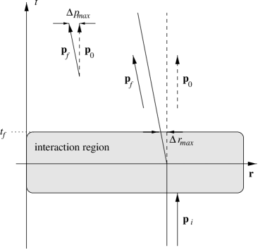
Fig. 1.—: Perturbed (solid line) versus unperturbed (dashed line) atomic trajectories. At time $t=t_{\rm f}$ where the atoms exit the interaction region with the diffraction grating, the maximum deviation in momentum (resp. in position) between the perturbed and unperturbed atomic trajectories is $\Delta p_{max}$ (resp. $\Delta r_{max}$).

To conclude, we point out some important features of the above perturbative method. First, the method clearly establishes an analogy between atomic diffraction by a weakly modulated optical potential, and light diffraction by a thin phase grating. Second, it is valid no matter the form of the unperturbed atomic trajectories, and thus identically applies to transmission and reflection gratings. Third, as will be shown in the following, it generally leads to analytical expressions of the diffraction amplitudes because $S_{1}$ only involves the unperturbed atomic trajectories which are often known analytically.

2.3 Calculation of the atomic diffraction spectrum

In a real experiment, atomic diffraction is observed at a distance from the grating much larger than its typical spatial modulation scale (generally of the order of a micron). As a result, the atomic wavefunction (2) evaluated just at the exit of the interaction region with the grating does not properly account for the observed diffraction pattern. In fact, it is necessary to propagate the atomic wavefunction in the far-field region for obtaining the appropriate diffraction spectrum. Here are summarized the main results of Appendix B, where the detailed derivation of the diffraction spectrum is presented.

For illustration purposes, we consider a two-dimensional geometry ($x$-$z$-plane) where atoms are incident from $z=-\infty$ with momentum ${\bf p}_{\rm i}$ on a diffraction grating with spatial modulation of period $a$ in the $x$ direction (the formalism can be generalized straightforwardly to a three-dimensional situation). Because of the periodicity of the grating, the atomic diffraction spectrum displays a discrete pattern. The diffraction orders are labeled by an integer number $n$ which denotes the momentum transfer $n\hbar q$ (with $q=2\pi/a$) from the grating to the atoms in the $x$ direction. It follows from energy conservation during the diffraction process that the atomic momentum ${\bf p}^{(n)}=(p_{x}^{(n)},p_{z}^{(n)})$ associated with the $n$-th diffraction order reads:

$$\left\{\begin{array}[]{rcl}p_{x}^{(n)}&=&p_{{\rm i},x}+n\hbar q\\ p_{z}^{(n)}&=&\sqrt{p_{\rm i}^{2}-(p_{x}^{(n)})^{2}}\end{array}\right.$$ (15)

where $p_{{\rm i},x}$ is the component of the incident atomic momentum along the $x$ axis. As shown in Appendix B, the diffraction amplitude $a_{n}$ associated with the $n$-th diffraction order can be evaluated from the value of the atomic wavefunction on a surface $z=z_{\rm f}$ located at the exit of the interaction region between the atoms and the light grating. More precisely, two situations can be distinguished depending on the way the atomic wavefunction is evaluated.

$\bullet$ Derivation from the WKB wavefunction. — In the case where the atomic wavefunction is evaluated following the WKB method (Sect. 2.2.1), the diffraction amplitudes are given by (see Appendix B):

$$a_{n}=\frac{1}{2a}\int_{0}^{a}{\rm d}x_{\rm f}\left[1+\frac{p_{{\rm f},z}(x_{\rm f})}{p_{z}^{(n)}}\right]\psi({\bf r}_{\rm f})\exp\left(-\frac{i}{\hbar}{\bf p}^{(n)}\cdot{\bf r}_{\rm f}\right)$$ (16)

where ${\bf r}_{\rm f}=(x_{\rm f},z_{\rm f})$ belongs to the ideally infinite surface $z=z_{\rm f}$ and $p_{{\rm f},z}(x_{\rm f})$ denotes the $z$-component of the atomic momentum associated with the classical perturbed trajectory ${\bf r}(t)$ satisfying the boundary conditions (4). It is important to note that equation (13) does not merely correspond to the Fourier transform of the atomic wavefunction after the interaction with the diffraction grating. A difference indeed arises due to the supplementary factor in square brackets, which accounts for the angle of inclination of the trajectories with respect to the normal of the surface $z=z_{\rm f}$.

$\bullet$ Derivation from the perturbation method. — In the case where the atomic wavefunction is evaluated following the perturbation method described in section 2.2.2, it is consistent to evaluate the diffraction amplitudes by substituting condition (11) into equation (13). As shown in Appendix B, this yields:

$$a_{n}=\frac{1}{a}\int_{0}^{a}{\rm d}x_{\rm f}\psi({\bf r}_{\rm f})\exp\left(-\frac{i}{\hbar}{\bf p}^{(n)}\cdot{\bf r}_{\rm f}\right)$$ (17)

which is the simple Fourier transform of the atomic wavefunction after the atom-grating interaction.

3 Illustration example: diffraction by a Gaussian standing wave.

We illustrate in this section the capabilities of our perturbation method by considering the well-known case of atomic diffraction by a Gaussian standing wave, leading to the nearly-resonant Kapitza-Dirac effect. We show that our method recovers the analytical expression for the diffraction orders [1, 2] at any incident angle, and we prove its equivalence to the Raman-Nath approximation. The validity condition (8) of the method is verified by comparison with numerical WKB calculations, and we show that the accepted validity conditon of the Ranam-Nath approximation can lead to inaccuracies in the evaluation of the phases of the diffraction amplitudes.

3.1 Calculation of the diffraction spectrum

Consider a two-dimensional geometry where an atomic beam of momentum ${\bf p}_{\rm i}$ crosses the waist $w$ of a Gaussian standing wave at the incidence angle $\theta$ ($\theta=0$ at normal incidence), and assume that the atomic kinetic energy is much larger than the height of the optical potential provided by the light field. The Lagrangian describing the atom dynamics thus takes the form (1) with:

$$\displaystyle L_{0} = \frac{1}{2}M{\bf\dot{r}}^{2}$$ (19)

$$\varepsilon V({\bf r}) = {\displaystyle\frac{\varepsilon}{\sqrt{2\pi}}}V_{1}\exp(-2z^{2}/w^{2})(1+\cos 2kx)$$ (20)

where $k=2\pi/\lambda$ is the wavevector associated with the laser wavelength $\lambda$. As described in section 2.2.2, the perturbation method is based on the evaluation of the action integral $S_{1}$ (Eq. (6b)) describing the phase-shift undergone by the atoms along their unperturbed trajectories ${\bf r}_{0}(t)=(x_{0}(t),z_{0}(t))$ which read:

$$\left\{\begin{array}[]{rcl}x_{0}(t)&=&x_{\rm i}+{\displaystyle\frac{p_{{\rm i},x}}{M}}t\\ z_{0}(t)&=&{\displaystyle\frac{p_{{\rm i},z}}{M}}t\end{array}\right.$$ (21)

The physical origin of the phase-shift can be visualized in figure 2a where we have projected the trajectories (16) onto the perturbation potenial (15b). More precisely, $S_{1}$ is evaluated by substituting equations (15b) and (16) into (6b). One thus gets:

$$S_{1}=-\frac{1}{2}V_{1}\tau(1+\beta_{KD}(\theta)\cos 2kx_{\rm i})$$ (22)

where $\tau=Mw/p_{{\rm i},z}$ is the typical interaction time between the atoms and the laser wave, and $\beta_{KD}(\theta)$ is a real parameter describing the amplitude of the phase modulation which depends on the incidence angle $\theta$ [11]:

$$\beta_{KD}(\theta)=\exp\left(-\frac{1}{2}(kw\tan\theta)^{2}\right)$$ (23)

Note that the Kapitza-Dirac incidence factor $\beta_{KD}$ decreases exponentially with the parameter $kw\tan\theta=k(p_{{\rm i},x}/M)\tau$, which corresponds to the dimensionless displacement of the atoms along the standing wave direction during the typical interaction time $\tau$. In particular, $\beta_{KD}=1$ (maximum value) at normal incidence, whereas $\beta_{KD}$ tends toward zero at grazing incidence (because of the spatial averaging of the potential modulation).

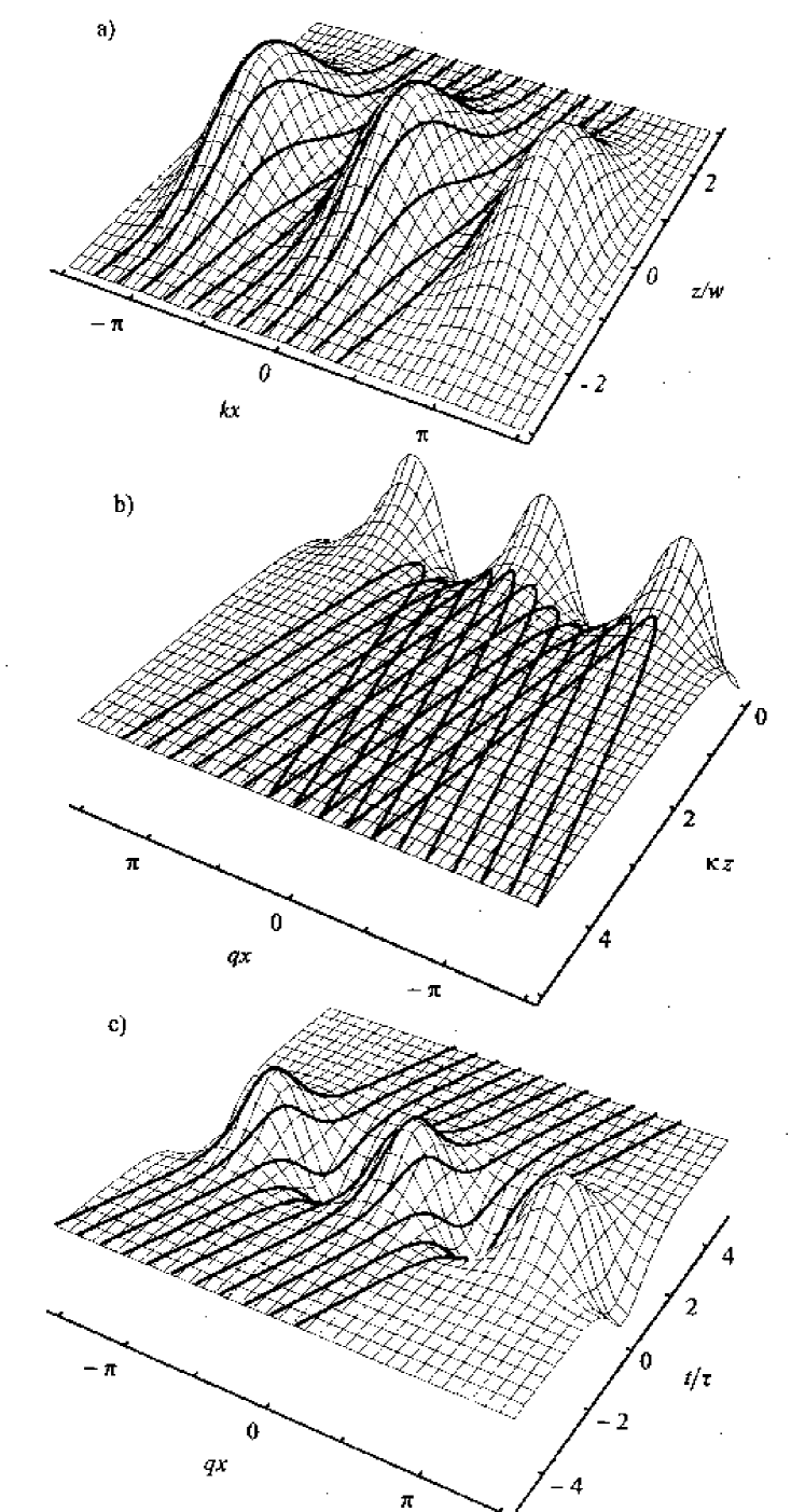
Fig. 2.—: Unperturbed atomic trajectories (bold lines) projected onto the perturbation potential $\varepsilon V$(mesh). The atomic diffraction process results from the spatially modulated phase-shift undergone by the atoms along their unperturbed trajectories where they interact with the perturbation potential. (a) Case of a Gaussian standing wave. (b) Case of an evanescent wave reflection grating ($x-z$ coordinates). Note that the potential surface only corresponds to the spatially modulated part of the optical potential, and thus takes both positive and negatibe values. (c) Same as figure 2b, but $x$-time coordinates. Note the analogy with the case of figure 2a.

Finally, using equations (17), (5) and (2), one obtains:

$$\psi(x_{\rm f},z_{\rm f})\propto\exp\left[-\frac{i}{2\hbar}\varepsilon V_{1}\tau\beta_{KD}(\theta)\cos[2k(x_{\rm f}-z_{\rm f}\tan\theta)]\right]$$ (24)

from which the populations of the diffraction orders follow straightforwardly (see Eq. (14)):

$$|a_{n}|^{2}=J_{n}^{2}\left[\beta_{KD}(\theta)\frac{\varepsilon V_{1}\tau}{2\hbar}\right]$$ (25)

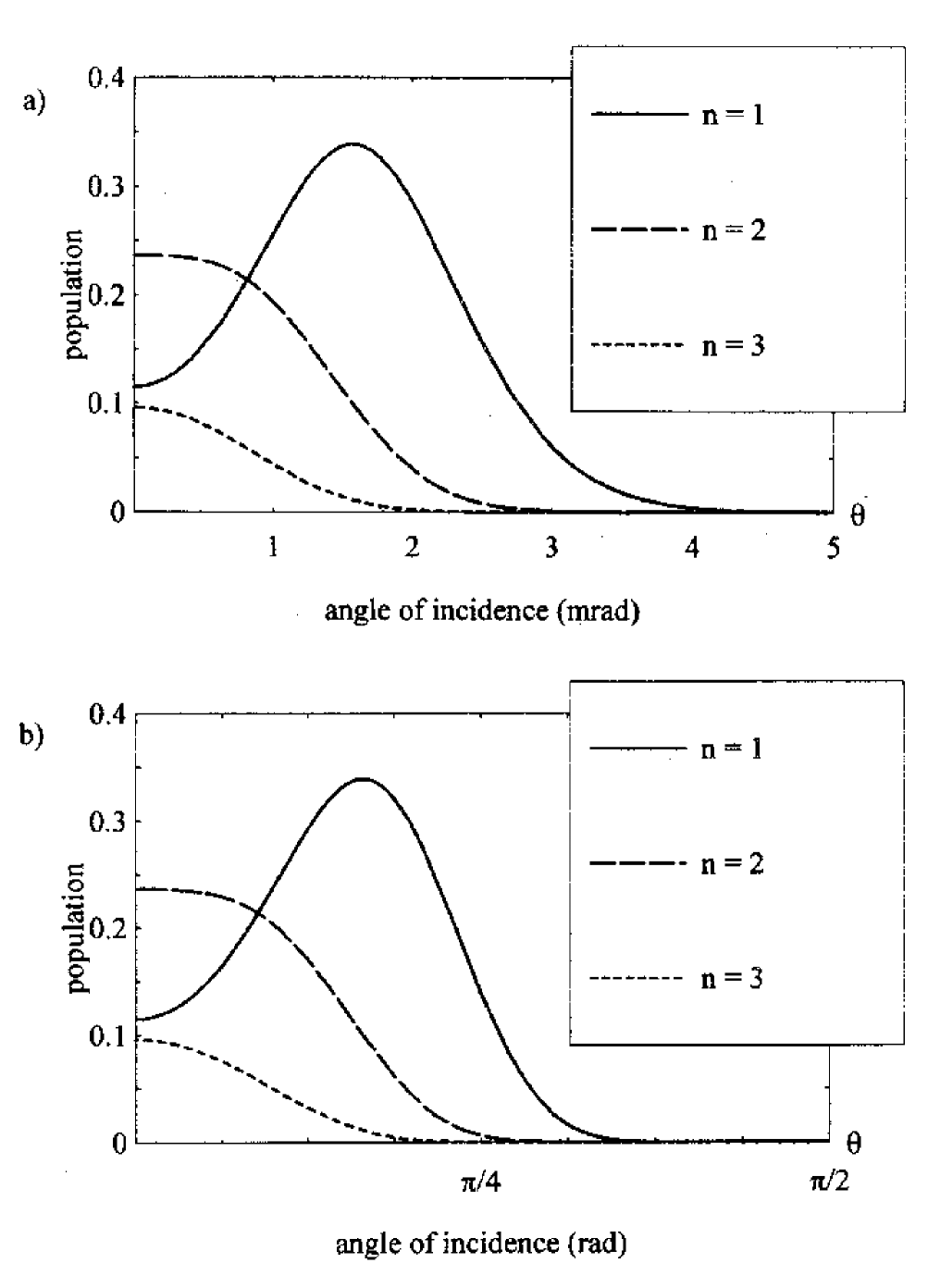
Fig. 3.—: Populations of the diffraction orders $n=1$-3 versus the incidence angle $\theta$ (diffraction orders $n$ and $-n$ are equally populated). (a) Case of a Gaussian standing wave transmission grating, with $w=100\lambda$ and $\varepsilon V_{1}\tau/(2\hbar)=3$. The diffraction pattern displays a dramatic dependence on $\theta$ on the scale of a few mrad. (b) By contrast, the evanescent wave reflection grating leads to a diffraction spectrum which varies much more smoothly with the incidence angle ($\kappa=q$, $\varepsilon p_{{\rm i},z}/(\hbar\kappa)=3$).

with $J_{n}$ the $n$-th Bessel function of integer order. Note that equation (20) exactly corresponds to the result derived by Martin et al. [12] using the Raman-Nath approximation. Note also that the estimate (20) is subject to the condition (11), which can be written in the form:

$$4n_{max}^{2}E_{R}\tau\ll\hbar$$ (26)

where $E_{R}=\hbar^{2}k^{2}/2M$ is the one-photon recoil energy, and $n_{max}$ is the maximum diffraction order, given approximately by $n_{max}\approx\beta_{KD}\frac{\varepsilon V_{1}\tau}{2\hbar}$.

We have represented in figure 3a the dependence of the populations of the three first diffraction orders as a function of the angle of incidence $\theta$, for a typical experimental value of the laser waist $w=100\lambda$ [12]. As reported in [12], the diffraction spectrum is found to display a dramatic sensitivity on the incidence angle on the scale of 5 mrad. This property results from the large value of $w$ used in figure 3a as well as in the experiment of reference [12] (see Eqs. (18) and (20).

3.2 Comparison with the Raman-Nath approximation

As shown above, the perturbation method allows us to recover exactly the analytical expression for the populations of the diffraction orders obtained using the Raman-Nath approximation. We show here that both approaches are actually equivalent in the case of a Gaussian standing wave diffraction grating.

Let us briefly recall the main features of the Raman-Nath approximation [2, 12]. This approach is based on the Schrödinger equation describing the interaction between fast atoms of incident momentum ${\bf p}_{\rm i}$ and the laser standing wave. In the interaction picture and after adiabatic elimination of the excited state, this equation reads:

$$i\hbar\partial_{t}\psi(x,t)=\left(-\frac{\hbar^{2}}{2M}\frac{\partial^{2}}{\partial x^{2}}+\varepsilon V[{\bf r}_{0}(t)]\right)\psi(x,t)$$ (27)

where $V$ is defined as in equation (15b) and ${\bf r}_{0}(t)$ as in equation (16). The atomic wavefunction is then Fourier-expanded as $\psi(x,t)=\sum_{n}a_{n}(t)e^{2inkx}$, and the diffraction amplitudes $a_{n}$ are found to satisfy:

$$i\dot{a}_{n} = \frac{\varepsilon}{2\sqrt{2\pi}}V_{1}\exp(-2t^{2}/\tau^{2})\times$$

$${}\times(a_{n-1}e^{2ikp_{{\rm i},x}/Mt}+2a_{n}+a_{n+1}e^{-2ikp_{{\rm i},x}/Mt})+4n^{2}E_{R}a_{n}.$$

Finally, the kinetic energy term in equation (23) is neglected compared to the average atom-field coupling, provided that the Raman-Nath condition is fulfilled:

$$4n_{max}^{2}E_{R}\ll\varepsilon\beta_{KD}V_{1}$$ (29)

Hence expression (20) is readily obtained.

In fact, the Raman-Nath approximation is equivalent to the Schrödinger equation (22) without the kinetic energy term, the solution of which:

$$\psi(x_{\rm f},t_{\rm f})\propto\exp\left(-\frac{i}{\hbar}\varepsilon\int_{t_{\rm i}}^{t_{\rm f}}{\rm d}tV[{\bf r}_{0}(t)]\right)$$ (30)

is rigorously equivalent to the result (19) obtained using the perturbation method. It is important to note however that despite the mathematical equivalence between the Raman-Nath approximation and the perturbation method, both approaches are associated with different validity conditions. Indeed, whereas condition (21) applies to the latter, the Raman-Nath approach is associated with equation (24) which can be rewritten using the expression of $n_{max}$ in the form:

$$2n_{max}E_{R}\tau\ll\hbar$$ (31)

Thus condition (21) is more severe than condition (26) by a factor of the order of $n_{max}$, which can be significantly larger than 1. We show in the following section that as far as the populations of the diffraction orders are concerned, conditions (21) and (26) are not easily distinguishable, but that equation (21) is actually more accurate than (26) for the estimate of the phases of the diffraction amplitudes.

3.3 Comparison with WKB calculations

Here we discuss in more details the validity of the perturbation method, by comparing it to the WKB treatment of atomic diffraction. In view of section 2, one can express the WKB wavefunction $\psi_{{\rm WKB}}$ in terms of the perturbed wavefunction $\psi_{{\rm pert}}$ as:

$$\psi_{{\rm WKB}}=\psi_{{\rm pert}}e^{i\delta\phi}$$ (32)

where in the limit of small deviations between the two approaches,

$$\delta\phi(x_{\rm f})\approx-\eta\sin^{2}[2k(x_{\rm f}-z_{\rm f}\tan\theta)].$$ (33)

Here $\eta=4n_{max}^{2}E_{R}\tau/\hbar$ is the small parameter from condition (21). As a result, from equation (27) and neglecting possible asymmetries in the diffraction, the diffraction spectrum derived from the perturbation method appears as the convolution of the WKB diffraction spectrum with the Fourier transform of the function:

$$\exp(i\delta\phi)=e^{-i\eta/2}\sum_{m=-\infty}^{+\infty}i^{m}J_{m}(\eta/2)\exp[4imk(x_{\rm f}-z_{\rm f}\tan\theta)]$$ (34)

which only displays even diffraction orders, and has a typical width $\delta m\approx\eta$.

In the limit $\eta\gg 1$ where condition (21) is not fulfilled, the convolution spectrum is large and thus the diffraction spectrum derived using the perturbation method differs significantly from the WKB spectrum. In contrast, in the limit $\eta\ll 1$ where the validity condition (21) is fulfilled, the convolution spectrum is narrow, and hence the perturbation method is a good approximation. Quantitatively, the second order expansion of function (29) reads:

$$\exp(i\delta\phi)\approx$$

$$\approx e^{i\eta/2}\left[1+i\frac{\eta}{2}\cos[4k(x_{\rm f}-z_{\rm f}\tan\theta)]-\frac{\eta^{2}}{8}\cos[8k(x_{\rm f}-z_{\rm f}\tan\theta)]-\frac{\eta^{2}}{16}\right].$$

As far as the phases of the diffraction amplitudes are concerned, the difference between the WKB and the perturbation method thus reduces to a global phase-factor $e^{i\eta/2}$. It is also possible to compare the populations of the diffraction orders using equation (30). After a straightforward calculation, one finds:

$$|a_{n,{\rm pert}}|^{2}-|a_{n,{\rm WKB}}|^{2}\approx-\frac{\eta^{2}}{16}\left[2J_{n}(J_{n}+J_{n-4}+J_{n+4})-(J_{n-2}+J_{n+2})^{2}\right]$$ (36)

where the argument of the Bessel functions is the same as in equation (20). Since the term in square brackets is typically of the order of unity, we see that the populations of the diffraction orders derived from the WKB and the perturbation method only differ by a fraction of $\eta^{2}$. It is important to note that the perturbation method, and hence the Raman-Nath approximation, is therefore much more accurate for the evaluation of the modulus square than for the estimate of the phases of the diffraction amplitudes.

We have performed numerical WKB calculations of the diffraction spectrum, and compared the results with those of the perturbation method. We have confirmed that in the case where condition (21) was fulfilled, the phases of the diffraction amplitudes actually differ by the amount $-\eta/2$. The populations of the diffraction orders were not clearly distinguishable as expected from the smallness of $\eta^{2}$. We have been particularly interested in the range of parameters where condition (26) was fulfilled, whereas condition (21) was not. In the parameter space that we have explored, we have observed that the populations of the diffraction orders were still given to a good approximation by equation (20), but that the phases of the diffraction amplitudes actually differed significantly from the WKB estimates.

In conclusion, it turns out that the validity of both the perturbation method and the Raman-Nath approximation are subject to one condition for the phases (Eq. (21)) and to another for the modulus square (Eq. (26)) of the diffraction amplitudes.

4 Diffraction by an evanescent wave reflection grating.

We consider in this section the atomic diffracton process associated with the reflection grating provided by an evanescent wave having a small standing wave component. Similar to the analogy between the Kapitza-Dirac effect and light diffraction by an acoustic wave, one might expect the evanescent wave reflection grating to be similar to the light diffraction grating produced by surface acoustic waves (where the periodic undulations of the free surface act as a surface grating). In fact, important differences arise between atom and conventional optics concerning the reflection gratings. First, the repulsive potentials of atomic mirrors typically vary on the scale of the optical wavelength, which is generally much larger than the de Broglie wavelength of the incident atoms. The situation is reversed in conventional optics where metallic or dielectric surfaces achieve spatial changes in the refractive index on a spatial scale much smaller than the optical wavelength. Second, from a geometrical optics point of view, atomic trajectories display properties different from those of light rays because of the nonzero atomic mass. For instance, the fact that an atom can be decelerated until its velocity is zero has no equivalent in conventional optics. We show here that in the semiclassical regime of reflection, the evanescent wave reflection grating is actually much more closely analogous to the transmission than to the reflection grating of conventional optics. More precisely, we prove that it is equivalent to the transmission grating produced by a standing laser wave having an Eckart profile ($\propto$ sech²). Analytical expressions for the populations of the diffraction orders at any incidence angle are obtained, and the experimental conditions for observing the diffraction spectrum in the thin phase grating limit are briefly discussed.

4.1 Calculation of the diffraction spectrum

Consider a two-dimensional geometry where an ensemble of laser-cooled atoms of momentum ${\bf p}_{\rm i}$ is incident on an evanescent wave reflection grating [3, 4] having a small standing wave component. Let $\theta$ denote the angle between ${\bf p}_{\rm i}$ and the normal of the mirror, and assume that the optical potential height provided by the evanescent wave is larger than the incident kinetic energy of the atoms. The Lagrangian describing the atom dynamics thus takes the form (1) with [13]:

$$L_{0} = \frac{1}{2}M{\bf\dot{r}}^{2}-V_{1}e^{-2\kappa z}$$ (38)

$$\varepsilon V({\bf r}) = \varepsilon V_{1}e^{-2\kappa z}\cos 2qx$$ (39)

where the wavevectors $\kappa$ and $q$ are typically of the order of the vacuum wavevector $k=2\pi/\lambda$ associated with the laser wavelength $\lambda$. Following the semiclassical perturbation method described in section 2.2.2, we first derive the unperturbed atomic trajectories ${\bf r}_{0}(t)=(x_{0}(t),z_{0}(t))$ which are given by [14]:

$$\left\{\begin{array}[]{rcl}x_{0}(t)&=&x_{\rm i}+{\displaystyle\frac{p_{{\rm i},x}}{M}}t\\[8.53581pt] z_{0}(t)&=&-{\displaystyle\frac{1}{2\kappa}}\ln\left[{\displaystyle\frac{p_{{\rm i},z}^{2}}{2MV_{1}}}\mbox{sech}^{2}(t/\tau)\right]\end{array}\right.$$ (40)

where $\tau=M/\kappa p_{{\rm i},z}$ it the typical reflection time of the atom on the evanescent wave mirror. Second, we evaluate the action integral $S_{1}$ (Eq. (6b)) by time-integration of the perturbation potential experienced by the atoms along their unperturbed trajectories (see Fig. 2). Using equations (32b) and (33), this potential is found to be:

$$\varepsilon V(t)=\varepsilon\frac{p_{{\rm i},z}^{2}}{2M}\cos[2q(x_{\rm i}+p_{{\rm i},x}/Mt)]\mbox{sech}^{2}(t/\tau).$$ (41)

By comparison with equations (15b) and (16), it clearly appears that equation (34) is analogous to the perturbation potential experienced by the atoms in the Kapitza-Dirac geometry discussed in section 3 with the following substitutions:

$$\left\{\begin{array}[]{l}V_{1}\to\sqrt{2\pi}p_{{\rm i},z}^{2}/2M\\ k\to q\\ w\to 1/\kappa\\ \exp(-2z^{2}/w^{2})\to\mbox{sech}^{2}(\kappa z).\end{array}\right.$$ (42)

This shows that in the limit of a small standing wave component, the evanescent wave reflection grating actually behaves as a transmission grating (see Fig. 2). This is because the optical potential associated with the evanescent wave varies very smoothly on the scale of the incident de Broglie wavelenght [15].

Substituting equation (34) into expression (6b), one readily obtains:

$$S_{1}=-\beta_{EW}(\theta)\frac{p_{{\rm i},z}}{\kappa}\cos 2qx_{\rm i}$$ (43)

where $\beta_{EW}(\theta)$ is the evanescent wave incidence parameter analogous to equation (18) given by:

$$\beta_{EW}(\theta)=\frac{\pi\tan\theta\,q/\kappa}{\sinh(\pi\tan\theta\,q/\kappa)}$$ (44)

which has a similar asymptotic behaviour as $\beta_{KD}$ (Eq.(18)) as $\theta$ tends toward 0 or $\pi/2$. Finally, using equations (36), (5), (2) and (14), it is straightforward to derive the populations of the diffraction orders which are found to read:

$$|a_{n}|^{2}=J_{n}^{2}\left(\varepsilon\beta_{EW}(\theta)\frac{p_{{\rm i},z}}{\hbar\kappa}\right).$$ (45)

Note that equation (38) is analogous to expression (20) with the replacements (35), as expected from the analogy with the Kapitza-Dirac effect. Note also that the argument of the Bessel functions (or equivalently the number of observable diffraction orders) is here proportional to the incident momentum in the $z$ direction in the case of the reflection grating, whereas it is inversely proportional to it in the case of the transmission grating (see Eq. (20)). This is because in the case of the transmission grating, the height of the perturbation potential is fixed and therefore the atomic phase-shift decreases with incident momentum because of the $1/p_{{\rm i},z}$-dependence of the interaction time $\tau$. By contrast, in the case of the reflection grating, the height of the effective perturbation potential experienced by the atoms is proportional to the square of the incident momentum, as shown by equation (35). For increasing momentum the increase of the potential height therefore overcomes the decrease of the interaction time, hence the phase-shift increases with $p_{{\rm i},z}$.

Similarly to the case of section 3, the accuracy of equation (38) is subject to condition (21) with $n_{max}\approx\varepsilon\beta_{EW}(\theta)p_{{\rm i},z}/\hbar\kappa$, with the restriction however that the semiclassical description of the reflection process be valid, i.e., $p_{{\rm i},z}\gg\hbar\kappa$ [14]. In fact, even though condition (21) is required for the accuracy of the phases of the diffraction amplitudes, equation (38) remains valid in a broader range of parameters given by a condition similar to equation (26).

We have represented in figure 3b the dependence of the populations of the three first diffracton orders as a function of the angle of incidence $\theta$, for typical experimental parameters. In contrast with the case of a Gaussian standing wave (Fig. 3(a)), the diffraction spectrum of the evanescent wave reflection grating does not exhibit a dramatic sensitivity on the incidence angle. This characteristic arises from the difference in the spatial extensions of the gratings along the $z$ direction ($w=100\lambda$ for the transmisson grating, $w=1/\kappa\approx\lambda/2\pi$ for the reflection grating).

4.2 Conditions for an experimental realization

Here we briefly discuss the experimental conditions required for the observation of atomic diffraction by an evanescent wave grating in the regime of small modulation of the optical potential investigated in the preceding section. Let us first examine the implications of the validity condition (21). Using the expression of $\tau$ and assuming that $\kappa\approx k$, one obtains as a first constraint:

$$p_{{\rm i},z}\gg 2n_{max}^{2}\hbar k.$$ (46)

In order to observe 5 diffraction orders, one thus has to achieve typically $p_{{\rm i},z}\approx 100\hbar\kappa$. Second, one has to take care of the absence of spontaneous emission events during the reflection process. As shown in [16], the spontaneous emission probability $P_{sp}$ per reflection reads:

$$P_{sp}=\frac{\Gamma}{\Delta}\frac{p_{{\rm i},z}}{\hbar\kappa}$$ (47)

where $\Gamma$ is the natural width of the excited state and $\Delta$ is the laser frequency detuning from resonance. In order to avoid spontaneous emission, one thus needs a laser detuning $\Delta\approx 10^{4}\Gamma$. Third, it is necessary to realize a sufficiently high optical potential barrier for reflecting the atoms, i.e., $V_{1}\approx 10^{4}E_{R}$. Because $V_{1}$ is inversely proportional to the detuning $\Delta$, this requires a large laser intensity, typically of the order of $10^{3}\,$W/mm² (case of rubidium atoms). This shows that such an experiment requires amplification techniques of the evanescent wave using either surface plasmons [17] or thin dielectric waveguides [18].

5 Application of the method to other experimental situations.

We have shown so far that the semiclassical perturbation method was a convenient tool for describing atomic diffraction by a weakly spatially modulated potential. We mention here possible extensions of the method to other situations of experimental interest.

$\bullet$ Atomic interferometry. — In atomic interferometry, it is often necessary to derive atomic phase-shifts due to small potentials, associated for example with a gravitational field or the rotation of the interferometer. In this situation, the expansion (6) can be used to calculate perturbatively the atomic phase-shifts using action integrals along the unperturbed atomic trajectories [19].
$\bullet$ Time-modulated potential. — Because the central point of the perturbation method consists in evaluating the time-integral of a perturbation potential experienced by an atom along its unperturbed trajectory, the method applies straightforwardly to the situation where an atom interacts with an optical potential having a sufficiently small time-modulated component. For an illustration in the case of a time-modulated evanescent wave optical potential, see reference [20].
$\bullet$ Multilevel atoms. — Certain experimental situations arise where the multilevel structure of the atoms plays an important role. For example, one can be interested in the atomic diffraction process by a Gaussian standing wave saturating the transition between a ground-state and a long-lived excited state. One can also consider a situation where the saturation of the optical transition is negligible, but where the Zeeman degeneracy of the ground-state is involved (e.g., an atom interacting with a standing wave displaying a polarization gradient). In such cases, the atomic state must be described by a spinor the components of which are associated with a given atomic internal state. However, in the case where the potential responsible for the mixing of the internal states can be considered as a small perturbation, it is possible to generalize our method and to derive the time-evolution of the atomic spinor by integration of the evolution operator associated with the perturbation potential along the unperturbed atomic trajectories [21].

6 Conclusion.

We have presented a semiclassical perturbation method which allows one to describe in a simple way the interaction between an atom and a potential having a small modulated component. This method is the analog in atom optics of the treatment of light interaction with thin phase objects in conventinal optics. It generally provides clear physical pictures as well as analytical descriptions of the interaction process. It consists in evaluating the atomic wavefunction by time-integration of the modulated potential along the unperturbed classical trajectories of the atoms. A validity condition of the method has been given and illustrated on the well-known Kapitza-Dirac effect, where the method has been proved to be equivalent to the Raman-Nath approximation. We have also used the perturbation method for deriving for the first time an analytical expression for the populations of the diffraction orders of an evanescent wave reflection grating at any incidence angle. This perturbation method should prove interesting in a broader range of experimental situations, as shown by its application to the treatment of atom interaction with time-modulated potentials [20].

Appendix A.

Semiclassical perturbative derivation of the atomic wavefunction.

In this appendix we derive equations (2) and (3) of section 2.1 for the semiclassical atomic wavefunction, as well as the perturbative expansion (6) of the integral (3).

A.1 Semiclassical derivation of the atomic wavefunction

For a time-independent Hamiltonian system, the quantum propagator can be represented by a Feynman path integral [22]. Thus, if at time $t=t_{\rm f}$, the atom is described by a plane wave of momentum ${\bf p}_{\rm i}$:

$$\psi({\bf r},t_{\rm i})=\exp\frac{i}{\hbar}({\bf p}_{\rm i}\cdot{\bf r})$$ (A.1)

then at time $t=t_{\rm f}$, the atomic wavefunction is given by the convolution product:

$$\psi({\bf r}_{\rm f},t_{\rm f})=\int d{\bf r}_{\rm i}K({\bf r}_{\rm f},t_{\rm f}|{\bf r}_{\rm i},t_{\rm i})\exp\left(\frac{i}{\hbar}{\bf p}_{\rm i}\cdot{\bf r}_{\rm i}\right)$$ (A.2)

with the Feynman propagator defined as the path-integral:

$$K({\bf r}_{\rm f},t_{\rm f}|{\bf r}_{\rm i},t_{\rm i})=\int_{({\bf r}_{\rm i},t_{\rm i})}^{({\bf r}_{\rm f},t_{\rm f})}{\cal D}[{\bf r}(t)]\exp\frac{i}{\hbar}\left(\int_{t_{\rm i}}^{t_{\rm f}}L({\bf r}(t),\dot{\bf r}(t)){\rm d}t\right).$$ (A.3)

The measure ${\cal D}[{\bf r}(t)]$ signifies that the integration is to be taken over all trajectories ${\bf r}(t)$ satisfying the boundary conditions:

$$\left\{\begin{array}[]{rcl}{\bf r}(t_{\rm i})&=&{\bf r}_{\rm i}\\ {\bf r}(t_{\rm f})&=&{\bf r}_{\rm f}\end{array}\right.$$ (A.4)

The semiclassical version of the quantum propagator (A.2) arises from a stationary-phase approximation. The path integral is then dominated by contributions from classical trajectories since these render the phase of the integrand stationary. The phase of the atomic wavefunction (times $\hbar$) is therefore given by the value of the generalized action:

$$S[{\bf r}(t),{\bf r}_{\rm i}]={\bf p}_{\rm i}\cdot{\bf r}_{\rm i}+\int_{t_{\rm i}}^{t_{\rm f}}L({\bf r}(t),\dot{\bf r}(t)){\rm d}t$$ (A.5)

for the specific initial point ${\bf r}_{\rm i}$ and the trajectory ${\bf r}(t)$ which fullfill the stationary-phase condition:

$$0=\delta S={\bf p}_{\rm i}\cdot\delta{\bf r}_{\rm i}+\delta{\bf r}\cdot\left.\frac{\delta L}{\delta\dot{\bf r}}\right|_{t_{\rm i}}^{t_{\rm f}}+\int_{t_{\rm i}}^{t_{\rm f}}\delta{\bf r}\cdot\left(\frac{\partial L}{\partial{\bf r}}-\frac{\rm d}{{\rm d}t}\frac{\partial L}{\partial\dot{\bf r}}\right){\rm d}t$$ (A.6)

for any small deviation ($\delta{\bf r}_{\rm i}$,$\delta{\bf r}(t)$) from the path of stationary phase. Because the boundary conditions (A.4) impose the relation:

$$\delta{\bf r}(t_{\rm i})=\delta{\bf r}_{\rm i}$$ (A.7)

it follows from (A.6) that:

$$\left\{\begin{array}[]{l}{\bf p}(t_{\rm i})={\displaystyle\frac{\partial L}{\partial\dot{\bf r}}}(t_{\rm i})={\bf p}_{\rm i}\\[8.53581pt] {\displaystyle\frac{\partial L}{\partial{\bf r}}}-{\displaystyle\frac{\rm d}{{\rm d}t}}{\displaystyle\frac{\partial L}{\partial\dot{\bf r}}}=0.\end{array}\right.$$ (A.8)

As expected, one finds that the stationary-phase trajectory ${\bf r}(t)$ is a classical trajectory (it is solution of the Euler-Lagrange equations of motion) which satisfies the boundary conditions (4). The semiclassical atomic wavefunction is hence given by equations (2) and (3) of section 2.1.

A.2 Perturbative expansion of the action integral

We consider the method described in section 2.2 for deriving the action integral (3) by an expansion in powers of the small parameter $\varepsilon$. In fact, only the second-order term is non-trivial: the zero-th order term $S_{0}$ corresponds to the absence of the modulated potential and hence to expression (6a), and equation (6b) arises from the fact that the term linear in $\varepsilon$ involving the nonperturbed Lagrangian $L_{0}$ vanishes by virtue of the stationary phase-condition (A.6) for the unperturbed trajectory ${\bf r}_{0}(t)$. In order to calculate the second-order term (6c), we have to expand both the boundary conditions (4) and the Euler-Lagrange equations of motion for the perturbed trajectory up to first order in $\varepsilon$. This yields the relations:

$$\left\{\begin{array}[]{l}0=\left(\dot{\bf r}_{1}\cdot{\displaystyle\frac{\partial}{\partial\dot{\bf r}}}+{\bf r}_{1}\cdot{\displaystyle\frac{\partial}{\partial{\bf r}}}\right)\left.{\displaystyle\frac{\partial L_{0}}{\partial\dot{\bf r}}}\right|_{{\bf r}={\bf r}_{0},\,\dot{\bf r}=\dot{\bf r}_{0},\,t=t_{0}}\\ \\ 0=\left(\dot{\bf r}_{1}\cdot{\displaystyle\frac{\partial}{\partial\dot{\bf r}}}+{\bf r}_{1}\cdot{\displaystyle\frac{\partial}{\partial{\bf r}}}\right){\displaystyle\frac{\partial L_{0}}{\partial{\bf r}}}-{\displaystyle\frac{\partial V}{\partial{\bf r}}}-{\displaystyle\frac{\rm d}{{\rm d}t}}\left(\dot{\bf r}_{1}\cdot{\displaystyle\frac{\partial}{\partial\dot{\bf r}}}+{\bf r}_{1}\cdot{\displaystyle\frac{\partial}{\partial{\bf r}}}\right)\left.{\displaystyle\frac{\partial L_{0}}{\partial\dot{\bf r}}}\right|_{{\bf r}={\bf r}_{0},\,\dot{\bf r}=\dot{\bf r}_{0}}\end{array}\right.$$ (A.9)

The second-order term of the action is equal to:

$$S_{2}={\bf p}_{\rm i}\cdot{\bf r}_{2}(t_{\rm i})+\int_{t_{\rm i}}^{t_{\rm f}}{\rm d}t\left({\bf r}_{2}\cdot{\displaystyle\frac{\partial L_{0}}{\partial{\bf r}}}+\dot{\bf r}_{2}\cdot{\displaystyle\frac{\partial L_{0}}{\partial\dot{\bf r}}}-{\bf r}_{1}\cdot{\displaystyle\frac{\partial V}{\partial{\bf r}}}+{\displaystyle\frac{1}{2}}\left({\bf r}_{1}\cdot{\displaystyle\frac{\partial}{\partial{\bf r}}}+\dot{\bf r}_{1}\cdot{\displaystyle\frac{\partial}{\partial\dot{\bf r}}}\right)^{2}L_{0}\right).$$ (A.10)

Note that all the quantities inside the integral are evaluated along the unperturbed trajectory. Finally, using (A.9), the Euler-Lagrange equation for ${\bf r}_{0}(t)$ and integrations by parts, equation (A.10) is readily simplified to get the result (6c).

Appendix B.

Calculation of the diffraction spectrum.

In this appendix we derive the expressions of the atomic diffraction amplitudes (13) and (14).

B.1 Quantum-mechanical integral theorem of Helmholtz and Kirchhoff

In a potential-free region of space, the wavefunction of an atom of kinetic energy $E$ satisfies the Schrödinger equation:

$$\nabla^{2}\psi+\frac{2ME}{\hbar^{2}}\psi=0.$$ (B.1)

Because equation (B.1) has the same form as the Helmholtz equation in electromagnetic theory, it is possible to use a quantum-mechanical version of the integral theorem of Helmholtz and Kirchhoff [23] to express the atomic wavefunction in the far-field region (which describes the diffraction pattern) from its value on a boundary surface $\Sigma$ located in the free-field region reached by the atoms after their interaction with the diffractron grating. One thus has:

$$\psi({\bf r})_{\rm farfield}=\frac{1}{4\pi}\int d\Sigma\,{\bf n}\cdot[G_{E}({\bf r},{\bf r}_{\rm f})\nabla\psi({\bf r}_{\rm f})-\psi({\bf r}_{\rm f})\nabla G_{E}({\bf r},{\bf r}_{\rm f})]$$ (B.2)

where ${\bf n}$ denotes the outward-pointing normal to the surface $\Sigma$, and ${\bf r}_{\rm f}$ corresponds to the endpoints of the classical trajectories along which the action integral (3) is calculated. The integral in equation (B.2) involves on one hand the quantum propagator $G_{E}({\bf r},{\bf r}_{\rm f})$ for a free particle of kinetic energy $E$, solution of:

$$\left[\nabla^{2}+\frac{2M}{\hbar^{2}}E\right]G_{E}({\bf r},{\bf r}_{\rm f})=-4\pi\delta({\bf r}-{\bf r}_{\rm f})$$ (B.3)

($\delta$ is the Dirac delta function), and on the other hand the value of the atomic wavefunction and its spatial derivative ${\bf n}\cdot\nabla\psi$ on the surface $\Sigma$. More precisely, $\nabla\psi$ is evaluated either from the WKB or the perturbation method using the relation:

$$\nabla\psi({\bf r}_{\rm f})=\frac{i}{\hbar}{\bf p}_{\rm f}({\bf r}_{\rm f})\psi({\bf r}_{\rm f})$$ (B.4)

where ${\bf p}_{\rm f}({\bf r}_{\rm f})$ is the local atomic momentum at the endpoint point ${\bf r}_{\rm f}$ of the classical trajectory. Note that whereas the direction of ${\bf p}_{\rm f}({\bf r}_{\rm f})$ generally depends on ${\bf r}_{\rm f}$, its modulus is constant, equal to that of the incident atomic momentum ${\bf p}_{\rm i}$ (because of energy conservation in the diffraction process).

B.2 Diffraction by a two-dimensional periodic grating

We consider here the particular case of a two-dimensional diffraction grating located in the $xOz$ plane (or equivalently a three-dimensional grating with translational invariance along the $y$-axis). We assume that the grating has a finite extent in the $z$-direction, but is infinite in the $x$-direction along which it is spatially modulated with the periodicity $a$. Using the notations of section 2, one thus has:

$$\forall x,\;\;V(x+a)=V(x)$$ (B.5)

It follows from equation (B.5) and the Bloch theorem that the atomic wavefunction will take the form:

$$\forall x,z\;\;\psi(x+a,z)=e^{ip_{{\rm i},x}a/\hbar}\psi(x,z)$$ (B.6)

with $p_{{\rm i},x}$ the component of the incident atomic momentum along the $x$-axis [24]. In order to take advantage if this property in the derivation of the diffraction spectrum, it is convenient to define the surface $\Sigma$ of equation (B.2) as a line $z=z_{\rm f}$ (${\bf n}=-{\bf e}_{z}$ is thus independent of ${\bf r}_{\rm f}$) and to express the two-dimensional quantum propagator $G_{E}({\bf r},{\bf r}_{\rm f})$ in the free-field region ($z>z_{\rm f}$) in the form [23]:

$$G_{E}({\bf r},{\bf r}_{\rm f})=i\int{\rm d}p_{x}\frac{1}{p_{z}}\exp\left(\frac{i}{\hbar}{\bf p}\cdot({\bf r}-{\bf r}_{\rm f})\right)$$ (B.7)

where $p_{z}=\sqrt{2ME-p_{x}^{2}}$ (the integration is restricted to the interval $|p_{x}|\leq\sqrt{2ME}$ because the evanescent wave components of the proagator do not contribute to the far-field wavefunction). Using equations (B.4), (B.6) and (B.7), and dividing the integration range of equation (B.2) into intervals of length $a$, one obtains:

$$\psi({\bf r})_{\rm farfield} = \frac{1}{4\pi\hbar}\sum_{n=-\infty}^{+\infty}\frac{1}{a}\int_{0}^{a}{\rm d}x_{\rm f}\int{\rm d}p_{x}\left[1+\frac{p_{{\rm f},z}(x_{\rm f})}{p_{z}}\right]\psi(x_{\rm f},z_{\rm f})\times{}$$ (B.8)

$${}\times\exp\left(\frac{i}{\hbar}n(p_{{\rm i},x}-p_{x})a\right)\exp\left(\frac{i}{\hbar}{\bf p}\cdot({\bf r}-{\bf r}_{\rm f})\right).$$

Using the relation:

$$\sum_{n=-\infty}^{+\infty}\exp\frac{i}{\hbar}n(p_{{\rm i},x}-p_{x})a=\hbar q\sum_{n=-\infty}^{+\infty}\delta(p_{x}-p_{{\rm i},x}-n\hbar q)$$ (B.9)

and expression (12) for the momenta associated with the different diffraction orders, equation (B.8) finally yields:

$$\psi({\bf r})_{\rm farfield}=\sum_{n=-\infty}^{+\infty}a_{n}\exp\left(\frac{i}{\hbar}({\bf p}^{(n)}\cdot{\bf r})\right)$$ (B.10)

where $a_{n}$ is the diffraction amplitude associated with the n-th diffraction order, which reads:

$$a_{n}=\frac{1}{2a}\int_{0}^{a}{\rm d}x_{\rm f}\left[1+\frac{p_{{\rm f},z}(x_{\rm f})}{p_{z}^{(n)}}\right]\psi({\bf r}_{\rm f})\exp\left(-\frac{i}{\hbar}{\bf p}^{(n)}\cdot{\bf r}_{\rm f}\right).$$ (B.11)

Even though equation (B.11) may be used to derive the atomic diffraction spectrum in the framework of the perturbation method, it seems more consistent to retain only the terms of (B.11) which correspond to the accuracy range of the method. As previously discussed in section 2.2.2 (Eq.(11)), in the validity domain of our semiclassical method one has:

$$\frac{\Delta p_{max}^{2}}{p_{\rm i}^{2}}\ll\frac{\hbar}{E\tau}\ll 1$$ (B.12)

and hence:

$$1-\left|\frac{p_{z}}{p_{\rm i}}\right|,1-\left|\frac{p_{z}^{(n)}}{p_{\rm i}}\right|\ll 1-\sqrt{1-\frac{\Delta p_{max}^{2}}{p_{\rm i}^{2}}}\approx\frac{\Delta p_{max}^{2}}{2p_{\rm i}^{2}}\ll 1$$ (B.13)

which yields:

$$\left|\frac{p_{{\rm f},z}}{p_{z}^{(n)}}-1\right|\ll 1$$ (B.14)

Finally, one obtains the expression of the diffraction amplitude for the atomic wavefunction derived using the perturbation method:

$$a_{n}=\frac{1}{a}\int_{0}^{a}{\rm d}x_{\rm f}\psi({\bf r}_{\rm f})\exp\left(-\frac{i}{\hbar}{\bf p}^{(n)}\cdot{\bf r}_{\rm f}\right)$$ (B.15)

which is merely the Fourier transform of the wavefunction evaluated on the line $z=z_{\rm f}$, after interaction with the diffraction grating.

References

-
[1]
Arimondo E., Lew H. and Oka T., Phys. Rev. Lett. 43 (1979)
753;
Delone G. A., Grinchuk V. A., Kuzmichev S. D., Nagaeva M. L., Kazantsev A. P. and Surdutovich G. C., Opt. Commun. 33 (1980) 149;
Gould P. L., Ruff G. A. and Pritchard D. E., Phys. Rev. Lett. 56 (1986) 827. -
[2]
Bernhardt A. F. and Shore B. W., Phys. Rev. A 23
(1981) 1290;
Martin P. J., Oldaker B. G., Miklich A. H. and Pritchard D. E., Phys. Rev. Lett. 60 (1988) 515;
Meystre P., Schumacher E. and Wright E. M., Ann. Phys. (Leipzig) 48 (1991) 141. -
[3]
Hajnal J. V., Baldwin K. G. H., Fisk P. T. H., Bachor H.-A. and
Opat G. I., Opt. Commun. 73 (1989) 331;
Christ M., Scholz A., Schiffer M., Deutschmann R. and Ertmer W., Opt. Commun. 107 (1994) 211. - [4] Deutschmann R., Ertmer W. and Wallis H., Phys. Rev. A 47 (1993) 2169.
-
[5]
Carnal O. and Mlynek J., Phys. Rev. Lett. 66
(1991) 2689;
Keith D. W., Ekstrom C. R., Turchette Q. A. and Pritchard D. E., Phys. Rev. Lett. 66 (1991) 2692. - [6] See, for example, Special issue on atom interferometry and atom optics, Appl. Phys. B 54, J. Mlynek, V. Balykin, P. Meystre Eds. (1992).
- [7] Kapitza P. L., Dirac P. A. M., Proc. Cambridge Philos. Soc. 29 (1933) 297.
- [8] See for example, the feature issue on the mechanical effect of light, J. Opt. Soc. Am B 2, N∘ 11 (1985).
- [9] Feynman R. P., Hibbs A. R., in Quantum Mechanics and Path Integrals (McGraw-Hill Inc., New-York, 1965).
- [10] Cohen-Tannoudji C., Cours du Collège de France (Paris, 1992), unpublished.
- [11] More generally, corresponds to the Fourier component of the beam profile at the wavevector . For instance, (the single-slit function) for the case of a rectangular profile of width .
- [12] Martin P. J., Gould P. L., Oldaker B. G., Miklich A. H. and Pritchard D. E., Phys. Rev. A 36 (1987) R2495.
- [13] We have neglected the distortion of the optical potential due to van der Waals interaction between the atom and the mirror surface.
- [14] Henkel C., Courtois J.-Y., Kaiser R., Westbrook C. and Aspect A., Laser Physics, 4 (1994) 1040.
- [15] Note that this property would not hold in the quantum regime of reflection achieved for incident atomic momentum of the order of , and for which the evanescent wave grating would behave as a hard potential barrier similar to a reflection grating in conventional optics [14].
- [16] Aminoff C. G., Steane A. M., Bouyer P., Desbiolles P., Dalibard J. and Cohen-Tannoudji C., Phys. Rev. Lett. 71 (1993) 3083.
-
[17]
Esslinger T., Weidemüller M., Hemmerich A. and Hänsch T. W.,
Opt. Lett. 18 (1993) 450;
Feron S., Reinhardt J., Le Boiteux S., Gorceix O., Baudon J., Ducloy M., Robert J., Miniatura C., Nic Chormaic S., Haberland H. and Lorent V., Opt. Commun. 102 (1993) 83. - [18] Kaiser R., Lévy Y., Vansteenkiste N., Aspect A., Seifert W., Leipold D. and Mlynek J., Opt. Commun. 104 (1994) 234.
- [19] For a more detailed discussion of such perturbation techniques in the field of atomic interferometry (see Ref. [10]).
- [20] Henkel C., Steane A. M., Kaiser R. and Dalibard J., J. Phys. II France 4 (1994) 1877.
-
[21]
For a similar approach see, for example, Macke B., Opt.
Commun. 28 (1979) 131;
Ishikawa J., Riehle F., Helmcke J. and Bordé C. J., Phys. Rev. A 49 (1994) 4794. - [22] Feynman R. P. and Hibbs A. R., Quantum Mechanics and Path Integrals (McGraw-Hill, New-York, 1965)
- [23] Nieto-Vesperinas M., in Scattering and Diffraction in Physical Optics (Wiley & Sons, New-York, 1991).
- [24] Wilkens M., Schumacher E. and Meystre P., Phys. Rev. A 44 (1991) 3130.