Theory and experiment of entanglement in a quasi-phase-matched two-crystal source

Abstract

We report new results regarding a source of polarization entangled photon-pairs created by the process of spontaneous parametric downconversion in two orthogonally oriented, periodically poled, bulk KTiOPO₄ crystals (PPKTP). The source emits light colinearly at the non-degenerate wavelengths of 810 nm and 1550 nm, and is optimized for single-mode optical fiber collection and long-distance quantum communication. The configuration favors long crystals, which promote a high photon-pair production rate at a narrow bandwidth, together with a high pair-probability in fibers. The quality of entanglement is limited by chromatic dispersion, which we analyze by determining the output state. We find that such a decoherence effect is strongly material dependent, providing for long crystals an upper bound on the visibility of the coincidence fringes of 41% for KTiOPO₄, and zero for LiNbO₃. The best obtained raw visibility, when canceling decoherence with an extra piece of crystal, was $91\pm 0.2\%$, including background counts. We confirm by a violation of the CHSH-inequality (${S=2.679\pm 0.004}$ at 55 s^-1/2 standard deviations) and by complete quantum state tomography that the fibers carry high-quality entangled pairs at a maximum rate of $55\times 10^{3}$ s^-1THz^-1mW^-1.

I Introduction

A nonlinear medium exposed to an optical field will occasionally emit several other photons. The phenomenon is known as spontaneous parametric downconversion (SPDC), and is frequently utilized for the production of photon-pairs. Such a pair can also become entangled in a certain degree of freedom if indistinguishability is ensured in all the remaining degrees of freedom. Many successful examples of direct creation of entangled photon-pairs Kwiat et al. (1995); Jennewein et al. (2000); Kurtsiefer et al. (2001a), post-selected entangled pairs Kiess et al. (1993); Tittel et al. (1999); Kim et al. (2000), and in-fiber generated pairs Takesue and Inoue (2004); Li et al. (2005a, b) can be given, already serving as an indispensable tool for quantum communication.

The source reported here uses two orthogonally oriented crystals, each emitting pairs of photons of a different polarization than the other. The different pairs are made indistinguishable, in our case by single-mode fibers, and therefore the individual photons of a single pair become directly entangled in polarization — an idea originally proposed by Hardy Hardy (1992) and realized in modified form by Kwiat et al. Kwiat et al. (1999). One problem with the original realization is that the crystals cannot be made too long, since the non-colinearity makes the two emission-cones non-overlapping. Another problem is that the crystals used generally emit into many spatial modes, which is not suitable for fiber-coupling. Using periodically poled crystals via quasi-phase matching Fiorentino et al. (2004); Mason et al. (2002); Tanzilli et al. (2002), it has been shown that colinear emission can be achieved very close to a single mode Ljunggren and Tengner (2005) (even in non-waveguiding structures), providing much greater overlap in the emission. Such a configuration also allows non-degenerate wavelengths to be generated.

Some desirable properties of sources to be used for quantum communication include: i) a high probability of photon-pairs to be collected into optical fibers; ii) a minimum number of false coincidences; iii) wavelength combinations that either suit efficient detection, match atomic transitions, or are well transmitted over long distances; iv) a narrow bandwidth that limits the effects of fiber dispersion ($\sim$ GHz) Halder et al. (2005) or can address atoms ($\sim$ MHz); v) a long coherence length that limits the need for precise interferometry; vi) small jitter in arrival-time of photons; vii) perfect correlations in all bases; and, ideally, viii) the source being compact enough to be put in a box, carried out of the lab, and be used, e.g., for quantum key distribution (QKD). Furthermore, for maximum security in QKD a strong requirement is to have neither more nor less than a single photon per gate pulse. In this respect, photon-pair sources have been shown to be good candidates compared to weak coherent pulses, potentially fulfilling properties i) and ii). Equally imperative for security in Ekert’s scheme Ekert (1991) is property vii), which expresses the wish for high visibility of entanglement in the presence of background detection, which implies the need to minimize dark counts and false coincidence counts.

In this work, we extend our previous results Pelton et al. (2004) regarding a PPKTP-based two-crystal source and try to address some of the anticipated features above. By emitting at non-degenerate wavelengths, the source exploits the highly efficient Si-based single-photon counters available in the near-infrared region and the low attenuation in fibers at telecom wavelengths. The shorter wavelength also matches the transmission bands of alkaline atoms, which makes the source suitable as part of a quantum memory Tanzilli et al. (2005); Konig et al. (2005). For our crystal configuration, we show how effects like chromatic dispersion enter the picture as problems to be dealt with. The source has been optimized for coupling into single-mode fibers following Ref. Ljunggren and Tengner (2005), where one can also find motivations for using long crystals to achieve a narrow bandwidth. An early example of a non-degenerate source is Ref. Ribordy et al. (2000), using energy-time entanglement. One reason for utilizing energy-time entanglement is to overcome the strong decoherence mechanism of polarization-states over fibers, and, for the same reason, we propose a scheme that combines time-multiplexed encoding on the telecom wavelength side Tittel et al. (2000) with polarization on the near-infrared side, altogether realizing a sort of hybrid-coded entanglement.

The article is organized as follows. In section II, we describe the main characteristics of the source. In section III, we derive the quantum state emitted by the two crystals in terms of frequency and polarization degrees of freedom, based on the quantum state of a single crystal derived in the Appendix. Following that, in section IV, we briefly show how to compensate for the effect of chromatic dispersion in the crystals, so as to assure indistinguishability, and, in section V, we present our experimental results showing the quality of the source, including results on quantum state tomography. In section VI, we discuss the future directions of a hybrid-coded source, and we end with a summary in section VII.

II A source of polarization entanglement

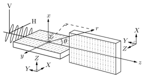
Figure 1: The source consists of two PPKTP crystals placed one after the other; the first creates a vertically (V) and the second a horizontally (H) polarized field. The laboratory coordinate system is drawn, as well as the crystal axes, $X$, $Y$, and $Z$, which refer to the polarization of the incoming and outgoing electromagnetic fields.

The source is depicted in Fig. 1, and consists of two orthogonally aligned bulk crystals placed one after the other. They each have the dimensions ${3\times 4.5\times 1}$ mm (${X,Y,Z}$), of which the second dimension defines the length, $L=4.5$ mm. The crystals are made of potassium titanyl phosphate, KTiOPO₄, and are periodical poled with the period $\Lambda=9.6\ \mu$m, chosen such that we have phase-matching for the signal at a wavelength of 810 nm, and the idler at 1550 nm, for a temperature $T=111^{\circ}$C determined by the Sellmeier equations of KTP Fan et al. (1987); Fradkin et al. (1999). The crystals are pumped by monochromatic and continuous wave laser light (p) at a wavelength of 532 nm, which is propagating in a Gaussian TEM₀₀ mode along the $z$-axis, producing a signal (s) and idler (i) field in the same direction and with the same polarization as the $Z$-component of the pump field ($Z_{\text{p}}Z_{\text{s}}Z_{\text{i}}$). Fig. 1 defines the laboratory axes and the crystals’ optical axes $X$, $Y$, and $Z$, oriented as shown. Both crystals will generate downconverted light if the pump polarization is oriented at $45^{\circ}$ to the horizontal (H) and vertical (V) axes. Following Ljunggren and Tengner (2005), we have optimized the focusing of the pump and the fiber-matched modes using the parameter $\xi=L/z_{R}$, where $L$ is the length of the crystal and $z_{R}$ is the Rayleigh range, such that the maximum amount of emission that is generated is collectible into single-mode fibers. The optimal values for our configuration are $\xi_{\text{p}}=1.3$, $\xi_{\text{s}}=2.0$, and $\xi_{\text{i}}=2.3$, respectively.

The use of single-mode fibers to collect the light will erase all spatial information that reveals from which crystal the photons came, except for the polarization degree of freedom. Therefore, each of the beams will interfere in the diagonal basis and get entangled in polarization. (Note that the spatial information is partly correlated with frequency via the phase-matching condition, and that indistinguishability could also be achieved via frequency filtering.) The resulting state is the Bell-state,

$$|\Phi^{\varphi}\rangle=\frac{1}{\sqrt{2}}\left(|\text{V}\rangle_{\text{s}}|\text{V}\rangle_{\text{i}}+e^{i\varphi}|\text{H}\rangle_{\text{s}}|\text{H}\rangle_{\text{i}}\right),$$ (1)

with a relative phase $\varphi$ that we can control. As in most cases, it is required that the probability of creating more than a single pair within a time determined by the coherence time of the photons, or the detector gate-time, whichever is longer, is negligible, and for moderate pump-powers and relatively short gate-times or wide bandwidths, this probability is very small, but not vanishing. Assuming a Poissonian distribution, the probability becomes $P_{n\geq 2}=1-(1+m)e^{-m}$, where $m=\Delta t_{\text{g}}\beta P_{\text{p}}\lambda_{\text{p}}/hc$ is the mean photon number in a single random gating. For a typical detector gate-time $\Delta t_{\text{g}}=5$ ns, pump-power $P_{\text{p}}=540\ \mu\text{W}$, and conversion efficiency $\beta=3\times 10^{-10}$ we get $m=2\times 10^{-3}$ and $P_{n\geq 2}=2\times 10^{-6}$.

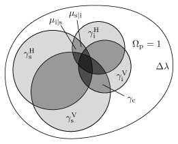
Figure 2: The figure shows a Venn diagram, which is used to illustrate the single coupling efficiencies $\gamma_{\text{s}}$ and $\gamma_{\text{i}}$, pair coupling $\gamma_{\text{c}}$, and conditional coincidences $\mu_{\text{s}|\text{i}}$ and $\mu_{\text{i}|\text{s}}$ as a fractional number representing the area of a set. The elements contained in a specific set represent photon pairs that are coupled into a fiber taken from the universal set of pairs, $\Omega_{\text{p}}$, which contains all pairs generated from the crystals (V or H) within the bandwidth of the detector filter $\Delta\lambda$. The set $\Omega_{\text{p}}$ is normalized to unity and represents perfect coupling. Maximum overlap of all sets is needed to generate the best entanglement in the fiber, which is represented by the darkest shaded area in the diagram (the union of all sets).

Fig. 2 will serve as an illustration of the problem of optimizing the focus of the pump-mode, and the fiber-matched modes with respect to two crystals. As a compromise, the pump-beam is focused at the interface between the crystals, in the anticipation that the profile of the generated emission exactly trails the profile of the pump-beam. However, numerical simulations with the software developed in Ljunggren and Tengner (2005) show that the waist of the emission will be shifted towards the center of each crystal, so that neither the vertically nor the horizontally polarized photons will couple perfectly into the fiber simultaneously. The figure shows the different types of coupling efficiencies represented as sets in a Venn-diagram, where each element of a set represents a photon pair generated by the crystals in some spatial mode. That is, the collection of all elements within each set defines which pairs are coupled into the fiber for some specific focusing condition, in such a way that the coupling efficiency corresponds to the total area of the set. The problem can be described in two parts: first, the need to overlap the matching modes of the signal and idler, represented by the coupling efficiencies $\gamma_{\text{s}}$ and $\gamma_{\text{i}}$, for each polarization separately (i.e. by optimizing the pair coupling $\gamma_{\text{c}}=\mu_{\text{i}|\text{s}}\gamma_{\text{s}}$, via the conditional coincidence $\mu_{\text{i}|\text{s}}$), and second, the need to overlap the vertically, $\gamma^{\text{V}}$, and the horizontally, $\gamma^{\text{H}}$, polarized photons for both the signal and idler. It is only in the intersection of all sets where entanglement exits, and any detection of photons outside of this set will limit the visibility in the $\pm 45^{\circ}$-basis (denoted here D/A-basis) by contributing to a mixed state. This picture is valid for many types of sources, and we believe that the coupling efficiencies in many cases in the literature are estimated in an incorrect way, as it is important to note that $\gamma_{\text{c}}\neq\gamma_{\text{s}}\gamma_{\text{i}}$ (especially in non-degenerate regimes). By this short discussion (see Tengner and Ljunggren (2005) for a comprehensive discussion), we hope to have illustrated that it is not necessarily best to optimize each arm individually to find the greatest coincidences, but rather, to simultaneously optimize both arms.

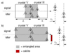
Figure 3: Color online. The figure illustrates the effects of chromatic dispersion resulting from the strong non-degeneracy of the signal and idler photons, with group refractive indices $n_{\text{g},\text{s}}$ and $n_{\text{g},\text{i}}$. a) A pair created at the end-facet of the V-crystal (black dots) will non-interactively pass through the H-crystal, after which the signal and idler wavepackets become separated by a time $\tau_{1}=(n_{\text{g},\text{s}}^{X}-n_{\text{g},\text{i}}^{X})L/c$ before hitting the detectors. As seen from the detectors’ viewpoint, for the same pair to instead have been created in the H-crystal (black dots), its wavepackets would necessarily need to have separated by the same amount, given by $\tau_{1}^{\prime}=(n_{\text{g},\text{s}}^{Z}-n_{\text{g},\text{i}}^{Z})b/c$, in order to interfere with (i.e. overlap with, or be indistinguishable from) the first case. (The superscripts refers to different polarization-axes.) Any pair created within the gray area (between black and white dots), are separated by a time $\tau\geq\tau_{1}=\tau_{1}^{\prime}$, and will always find a corresponding position in the orthogonal crystal to interfere with, according to the detectors; however, all the pairs from the white area of either crystal will be distinguishable in time from any pair of the other crystal, i.e. the wavepackets are non-overlapping due to different dispersions, and contribute therefore to a mixed output state. b) If we put a birefringent plate of thickness $d$ in one of the arms, the time-separation for a pair created at the end-facet of the V-crystal is reduced to $\tau_{2}=(n_{\text{g},\text{s}}^{X}-n_{\text{g},\text{i}}^{X})L/c+(1-n_{\text{g},\text{c}}^{e})d/c<\tau_{1}$, for which some $d$ equals the time-separation of an interfering position at the end-facet of the H-crystal, $\tau_{2}=-(1-n_{\text{g},\text{c}}^{o})d/c$. Consequently, all H and V-pairs now show “self-interference”, and a pure output state is created. Note that two pairs created within the coherence time of the pump (which needs to be longer than $L$) are always coherent, ignoring dispersion.

As we have mentioned, the different polarizations need to interfere, and therefore a major concern is that they are not distinguishable by time information, noting the limited extent of the photon wave-packets. For long crystals, the photon pairs will separate by chromatic dispersion, due to the very different group velocities between the strongly non-degenerate signal and idler. This will occur to a degree that is different for pairs created in the first crystal than for pairs created in the second, because the pairs from the first crystal also need to pass through the second. The differences in group velocities between signal and idler are not the same for light polarized along the $Z$-axis and the $X$-axis, implying that not all pairs, created along the length of either crystal, will find any (possibly) generated pairs to interfere with from the other crystal. Some photon-pairs will therefore be distinguishable by temporal information. See Fig. 3 for an illustration. We would like to point out that, while this chromatic two-photon dispersion effect is reminiscent of the “two-photon dispersion” effects discussed in Kwiat et al. (1995) or Kuklewicz et al. (2004), it does not have the same origin, although the current effect can also be compensated for by an extra piece of crystal. The chromatic effect comes as an disadvantage when placing the crystals adjacent to each other, and could in principle be avoided by an “interferometric” solution Kim et al. (2000); Fiorentino et al. (2004), in which the pump beam splits into two separate arms, impinges onto each of the crystals, or onto a single crystal but in opposite directions, and recombines on a beam-splitter. Still, we believe the current solution requires fewer optics, is easier to align, and can be made more compact.

The previous discussion gave a limited, although intuitive, understanding of the origin of a mixed state, but, as we will show in the next section, a mathematical derivation will give additional insights into how the effect of decoherence is affected by the group velocities.

III The two-crystal two-photon quantum state

In this section, we derive the output state from the two-crystal source in terms of the frequency and polarization degrees of freedom $|\bm{\epsilon}\rangle\otimes|\bm{\chi}_{i,j}^{\phantom{1}}\rangle$, where $i,j=\{1=``\text{V}",2=``\text{H}"\}$ denotes the polarizations. Emission from each of the crystals, V and H, will thus be represented by $|\bm{\chi}_{11}\rangle$ and $|\bm{\chi}_{22}\rangle$, respectively, according to Eq. (39) of the Appendix and Fig. 1. As just described, the vertical light will be subject to dispersion upon its passing through the second crystal. We will formulate this mathematically by introducing a unitary transform acting on the states. The eigenequation which describes the transformation $U_{L}$ on the state of the first crystal, when it passes through the second crystal, is

$$U_{L}|\bm{\chi}_{11}\rangle =e^{i(k_{\text{s}}L+k_{\text{i}}L)}|\bm{\chi}_{11}\rangle$$

$$=e^{i(n_{\text{s}}^{X}\omega_{0\text{s}}+n_{\text{i}}^{X}\omega_{0\text{i}}+(n_{\text{g},\text{s}}^{X}-n_{\text{g},\text{i}}^{X})\epsilon)L/c}|\bm{\chi}_{11}\rangle,$$ (2)

where the length of the crystal, $L$, enters the phase term, together with the frequency $\epsilon$. With reference to the Appendix A, and Eq. (39), we can then express the output state of each crystal as

$$|\Psi_{11}\rangle =\frac{1}{B}\int\!\!\text{d}\epsilon\>U_{L}U(\epsilon)\>|\bm{\epsilon}\rangle\otimes|\bm{\chi}_{11}\rangle,$$

$$|\Psi_{22}\rangle =\frac{1}{B}\int\!\!\text{d}\epsilon\>U(\epsilon)\>e^{in_{\text{p}}^{X}\omega_{\text{p}}L/c}\>|\bm{\epsilon}\rangle\otimes|\bm{\chi}_{22}\rangle,$$ (3)

where an extra phase-term has been added to the pump field in the second crystal due to the pump field passing through the first crystal, $U(\epsilon)$ is the state amplitude, and $B$ is a normalization constant. The sum of these two kets will give us the combined two-crystal two-photon state,

$$|\Psi^{\epsilon}\rangle =|\Psi_{11}\rangle+|\Psi_{22}\rangle$$

$$=\frac{1}{B}\int\!\!\text{d}\epsilon\>\Big{[}U_{L}U(\epsilon)|\bm{\epsilon}\rangle\otimes|\bm{\chi}_{11}\rangle$$

$$\qquad+\>U(\epsilon)e^{in_{\text{p}}^{X}\omega_{\text{p}}L/c}|\bm{\epsilon}\rangle\otimes|\bm{\chi}_{22}\rangle\Big{]}$$

$$=\frac{1}{B}\int\!\!\text{d}\epsilon\sum\limits_{i,j=1}^{2}c_{ij}V_{ij}(\epsilon)\>|\bm{\epsilon}\rangle\otimes|\bm{\chi}_{ij}\rangle,$$ (4)

where we have introduced $V_{11}(\epsilon)=\frac{1}{B}U_{L}U(\epsilon)$, $V_{22}(\epsilon)=\frac{1}{B}U(\epsilon)e^{in_{\text{p}}^{X}\omega_{\text{p}}L/c}$, and the coefficients $c_{ij}=1/\sqrt{2}$ for $i=j$, and $c_{ij}=0$ for $i\not=j$, normalized such that $|c_{11}|^{2}+|c_{22}|^{2}=1$.

We can now form the two-photon density matrix

$$\bm{\rho}^{\epsilon} =|\Psi^{\epsilon}\rangle\langle\Psi^{\tilde{\epsilon}}|$$

$$=\frac{1}{B^{2}}\iint\!\!\text{d}\epsilon\>\text{d}\tilde{\epsilon}\!\!\sum\limits_{i,j,k,l=1}^{2}\!\!c_{ij}c_{kl}^{\ast}V_{ij}(\epsilon)V_{kl}^{\ast}(\tilde{\epsilon})\>|\bm{\epsilon}\rangle\langle\tilde{\bm{\epsilon}}|\otimes|\bm{\chi}_{ij}\rangle\langle\bm{\chi}_{kl}|,$$ (5)

from which we would like to remove the frequency information. For that, we need to note that we could, in principle, measure the frequency of the photons at a resolution much smaller than the bandwidths of the filters. The resolution is given by a wavelength bandwidth $\Delta\lambda_{\text{res}}$, which is set by the timing information $\Delta t_{\text{gate}}$ of the detectors ($\Delta\lambda_{\text{res}}=\lambda^{2}/c\Delta t_{\text{gate}}<8$ pm for $\Delta t_{\text{gate}}>1$ ns). Therefore, it is appropriate to take the partial trace over the frequency mode:

$$\bm{\rho} =\text{Tr}_{\epsilon}[\>|\bm{\epsilon}^{\prime}\rangle\langle\bm{\epsilon}^{\prime}|\>\bm{\rho}^{\epsilon}]=\int\limits_{-\infty}^{\infty}\!\!\text{d}\bm{\epsilon}^{\prime}\langle\bm{\epsilon}^{\prime}|\bm{\rho}^{\epsilon}|\bm{\epsilon}^{\prime}\rangle$$

$$=\frac{1}{B^{2}}\sum\limits_{i,j,k,l=1}^{2}\!c_{ij}c_{kl}^{\ast}\int\!\!\text{d}\epsilon^{\prime}V_{ij}(\epsilon^{\prime})V_{kl}^{\ast}(\epsilon^{\prime})\>|\bm{\chi}_{ij}\rangle\langle\bm{\chi}_{kl}|.$$ (6)

Let $\rho_{ijkl}$ denote the elements of the density matrix, of which the only non-zero ones become

$$\rho_{1122} =c_{11}c_{22}^{\ast}\frac{1}{B^{2}}\int\!\!\text{d}\epsilon^{\prime}U_{L}U(\epsilon^{\prime})\>U^{\ast}(\epsilon^{\prime})e^{-in_{\text{p}}^{X}\omega_{\text{p}}L/c}$$

$$=\frac{1}{2}\frac{\chi_{2}^{2}\>f_{1}^{2}E_{0}^{2}L^{2}}{\hbar^{2}B^{2}}$$

$$\quad\times\>\int\!\!\text{d}\epsilon^{\prime}\>|A_{\text{s}}(\epsilon^{\prime})|^{2}|A_{\text{i}}(\epsilon^{\prime})|^{2}$$

$$\quad\times\>e^{-in_{\text{p}}^{X}\omega_{\text{p}}L/c}\>e^{i(n_{\text{s}}^{X}\omega_{0\text{s}}\>+\>n_{\text{i}}^{X}\omega_{0\text{i}}\>+\>(n_{\text{g},\text{s}}^{X}-n_{\text{g},\text{i}}^{X})\epsilon^{\prime})L/c}$$

$$\quad\times\>\text{sinc}^{2}\left[\frac{L\epsilon^{\prime}}{2c}(n_{\text{g},\text{s}}^{Z}-n_{\text{g},\text{i}}^{Z})\right]\>$$

$$=\rho_{2211}^{\ast}$$ (7)

and

$$\rho_{1111} =\rho_{2222}=\frac{1}{2}.$$ (8)

The off-diagonal element, which describes the degree of coherence in the entangled state, can be further simplified and identified as a Fourier transform:

$$\rho_{1122} =\frac{1}{2}\>e^{-in_{\text{p}}^{X}\omega_{\text{p}}L/c}\>e^{i(n_{\text{s}}^{X}\omega_{0\text{s}}+n_{\text{i}}^{X}\omega_{0\text{i}})L/c}$$

$$\quad\times\>\int\!\!\text{d}\epsilon^{\prime}\>g(\epsilon^{\prime})\>e^{i\tau_{X}^{\phantom{1}}\epsilon^{\prime}}\>\text{sinc}^{2}(\frac{\tau_{Z}^{\phantom{1}}}{2}\epsilon^{\prime}),$$ (9)

where

$$g(\epsilon^{\prime}) =\frac{\chi_{2}^{2}\>f_{1}^{2}E_{0}^{2}L^{2}}{\hbar^{2}B^{2}}|A_{\text{s}}(\epsilon^{\prime})|^{2}|A_{\text{i}}(\epsilon^{\prime})|^{2},$$

$$\tau_{X}^{\phantom{1}} =(n_{\text{g},\text{s}}^{X}-n_{\text{g},\text{i}}^{X})L/c,$$

$$\tau_{Z}^{\phantom{1}} =(n_{\text{g},\text{s}}^{Z}-n_{\text{g},\text{i}}^{Z})L/c.$$ (10)

In Fig. 4,

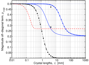
Figure 4: Color online. The off-diagonal term, Eq. (9), of the generated density matrix plotted versus crystal length, which corresponds to the visibility of entanglement via the relation $V=2\rho_{1122}$. Solid line: PPKTP-crystal with 10 nm idler filter. Dots over solid line: PPKTP with 1 nm idler filter. Dash-dotted line: PPLN or PPMgOLN with 10 nm idler filter. Dashed line: PPKTP at optimal fiber coupling using the idler fiber’s own filtering. Diamond: experimental value for $L=4.5$ mm using PPKTP and with a 10 nm idler filter. Solid point: experimental value for $L=4.5$ mm using PPKTP and with a dispersion canceling calcite plate of thickness $d=0.86$ mm.

we have plotted the result of Eq. (9) versus the length of the crystals using different crystal materials to generate 810 and 1550 nm. We observe that the dispersion in long, periodically poled LiNbO₃ (PPLN) crystal materials completely suppresses the $\rho_{1122}$ term, and thereby the entanglement. For PPKTP this is not the case, and if we search for $\rho_{1122}$ in the limit of an infinitely long crystal we find that

$$\lim\limits_{L\to\infty}|\rho_{1122}| =\left\{\begin{array}[]{ll}1-\frac{\tau_{X}^{\phantom{1}}}{\tau_{Z}^{\phantom{1}}}&\text{if}\quad\tau_{X}^{\phantom{1}}<\tau_{Z}^{\phantom{1}}\\ 0&\text{if}\quad\tau_{X}^{\phantom{1}}\geq\tau_{Z}^{\phantom{1}},\end{array}\right.$$ (13)

which, for PPKTP leads to $\rho_{1122}=0.203$, implying still a visibility of entanglement (i.e. of the second-order interference fringes) of $40.6\%$. The different results stem from the material-specific relation between $\tau_{X}^{\phantom{1}}$ and $\tau_{Z}^{\phantom{1}}$. If the material is more strongly dispersive for polarizations along the $Z$-axis than the $X$-axis, then the off-diagonal term will be bounded below by a non-vanishing value; otherwise, the off-diagonal term will approach zero. As expected, we found that all numbers increase as we go closer to having degenerate wavelength pairs. We also note that the bandwidth of the frequency filter affects the shape of the curve; a narrower bandwidth increases the extent of the temporal coherence and provides a greater overlap between wave-packets, leading to an arbitrarily increased $\rho_{1122}$. Emission that is optimally coupled into single-mode fibers will automatically be filtered also in frequency, since the frequency is correlated to spatial information via the phase-matching conditions Ljunggren and Tengner (2005), and for long PPKTP crystals, in such a case, the minimum value of $\rho_{1122}$ equals 0.266 ($V=53.2\%$).

IV Decoherence cancellation

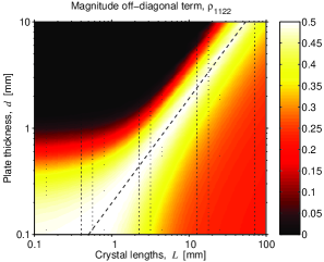
Figure 5: Color online. The off-diagonal term, Eq. (16), plotted versus the crystal lengths, $L$, and the thickness, $d$, of a dispersion-canceling calcite plate, using PPKTP with a 10 nm idler filter. The dashed line represents perfect cancellation.

We will now briefly show how the pure state, $|\Phi^{\varphi}\rangle$ in Eq. (1), can be fully regained, for generation in long crystals, by inserting a highly birefringent crystal plate into one of the arms. The eigenequations for each polarization state propagating through such a crystal plate become

$$U_{C}|\bm{\chi}_{1j}\rangle =e^{ik_{\text{c}}d}|\bm{\chi}_{1j}\rangle$$

$$=e^{i(n_{\text{c}}^{o}\omega_{0\text{i}}-n_{\text{g},\text{c}}^{o}\epsilon)d/c}|\bm{\chi}_{1j}\rangle,$$

$$U_{C}|\bm{\chi}_{2j}\rangle =e^{ik_{\text{c}}d}|\bm{\chi}_{2j}\rangle$$

$$=e^{i(n_{\text{c}}^{e}\omega_{0\text{i}}-n_{\text{g},\text{c}}^{e}\epsilon)d/c}|\bm{\chi}_{2j}\rangle,$$ (14)

with the density matrix after the plate becoming

$$\bm{\rho}^{\epsilon}(d) =U_{C}\bm{\rho}^{\epsilon}U_{C}^{\dagger}.$$ (15)

Repeating Eqns. (5) to (9), we arrive at

$$\rho_{1122} =\frac{1}{2}\>e^{-in_{\text{p}}^{X}\omega_{\text{p}}L/c}\>e^{i(n_{\text{s}}^{X}\omega_{0\text{s}}+n_{\text{i}}^{X}\omega_{0\text{i}})L/c}$$

$$\quad\times\>e^{i(n_{\text{c}}^{o}\omega_{0\text{i}}-n_{\text{c}}^{e}\omega_{0\text{i}})d/c}$$

$$\quad\times\>\int\!\!\text{d}\epsilon^{\prime}\>g(\epsilon^{\prime})\>e^{i(\tau_{X}^{\phantom{1}}-\kappa)\epsilon^{\prime}}\>\text{sinc}^{2}(\frac{\tau_{Z}^{\phantom{1}}}{2}\epsilon^{\prime}),$$ (16)

where $g(\epsilon^{\prime}),\tau_{X}^{\phantom{1}}$, and $\tau_{Z}^{\phantom{1}}$ is defined by Eq. (10), and where

$$\kappa =(n_{\text{g},\text{c}}^{o}-n_{\text{g},\text{c}}^{e})d/c.$$ (17)

Now, if $d$ is chosen such that $\kappa=\tau_{X}^{\phantom{1}}$, it means that we have perfectly canceled the decoherence and retrieved a pure state. Hence,

$$\rho_{1122}=\rho_{2211}^{\ast}=\rho_{1111}=\rho_{2222}=\frac{1}{2}.$$ (18)

Note that, by adjusting $d$ and tilting the plate (affecting $\varphi$) our source can prepare any arbitrary mixed state of the kind $\bm{\rho}=V|\bm{\Phi}^{\varphi}\rangle\langle\bm{\Phi}^{\varphi}|+(1-V)\bm{\rho}_{m}$, where $\bm{\rho}_{m}=\frac{1}{2}(|\bm{\chi}_{11}\rangle\langle\bm{\chi}_{11}|+|\bm{\chi}_{22}\rangle\langle\bm{\chi}_{22}|)$, and $V$ is the visibility. Fig. 5 shows a plot of $\rho_{1122}$ versus $L$ and $d$.

V Experimental results

The experimental setup used when characterizing the source’s output state is shown in Fig. 6. As a pump, we use a frequency-doubled Nd:YAG laser emitting approximately 60 mW in the TEM₀₀ mode at 532 nm, which can be variably attenuated. Its $M_{\text{p}}^{2}$ value was measured to be 1.06. After a band-pass filter (BP532) that removes any remaining infrared light, we “clean up” the polarization using a polarizing beam-splitter (PBS). The polarization is controlled by a half-wave plate (HWP) and a quarter-wave plate (QWP) in front of the crystal. The pump beam is focused onto the crystal using an achromatic doublet lens ($f_{\text{p}}=50\ \text{mm}$), which introduces a minimal amount of aberrations, so as not to destroy the low $M^{2}$–value. The QWP is set to undo any polarization elliptisation effects caused by the lens, and fluorescence caused by the same lens is removed by a Schott-KG5 filter (SP).

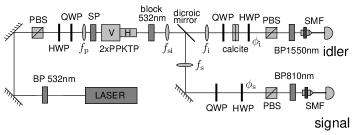
Figure 6: Experimental setup used to measure the density matrix. PBS: polarizing beam-splitter, HWP: half-wave plate, QWP: quarter-wave plate, SP: short-pass filter, BP: band-pass filter, SMF: single-mode fiber.

Table 1: Three runs at different alignments and pump powers, showing the coupling efficiencies, photon rates in fibers, conversion efficiency, and the production rate of the system.

$P_{\text{p}}$ [mW]	$\gamma_{\text{s}}$	$\gamma_{\text{i}}$	$\gamma_{\text{c}}$	$\mu_{\text{i}|\text{s}}$	$\sigma$	$R_{\text{s}}$ [s-1]	$R_{\text{i}}$ [s-1]	$R_{\text{p}}$ [s-1]	$R_{\text{c}}$ [s-1]	$\beta$	$R_{\text{c}}^{\text{prod}}$ [​ s-1THz-1mW-1]
$\rule{0.0pt}{12.91663pt}60$	0.32	0.79	0.11	0.12	0.34	$2.32\times 10^{6}$	$2.39\times 10^{6}$	$8.61\times 10^{6}$	$274\times 10^{3}$	$5\times 10^{-11}$	$5.0\times 10^{3}$
$4.5$	0.32	0.56	0.10	0.11	0.32	$167\times 10^{3}$	$121\times 10^{3}$	$617\times 10^{3}$	$19\times 10^{3}$	$5\times 10^{-11}$	$4.6\times 10^{3}$
$0.54$	0.46	0.38	0.22	0.27	0.57	$100\times 10^{3}$	$195\times 10^{3}$	$450\times 10^{3}$	$27\times 10^{3}$	$3\times 10^{-10}$	$55\times 10^{3}$

The next components are the two PPKTP crystals, which are heated in an oven to a temperature $T\approx 100^{\circ}$. After the crystals, we block the pump light with a 532 nm band-stop filter, and the signal and idler emission is focused by achromatic doublet lenses. To separate the 810 nm and 1550 nm emission, we use a dichroic mirror made for a $45^{\circ}$ angle of incidence. The first lens ($f_{\text{s}\text{i}}=30\ \text{mm}$) is common to both signal and idler, and its task is to refocus the beams somewhere near the dichroic mirror. The next two lenses ($f_{\text{s}}=60\ \text{mm}$ and $f_{\text{i}}=40\ \text{mm}$) collimate each beam, which are then focused into the fiber tips (with the mode field diameters being $\text{MFD}_{810}=5.5\ \mu\text{m}$ and $\text{MFD}_{1550}=10.4\ \mu\text{m}$) using aspherical lenses with $f=11\text{\ mm}$. Next, we use quarter-wave plates (QWP), half-wave plates (HWP), and polarizing beam-splitters (PBS) in each arm to analyze the state. In the idler arm, we also place the tiltable cancellation plate, which is made of calcite. In front of the fiber couplers, we have first Schott-RG715/RG1000 filters to block any remaining pump light, and then interference filters (BP) of 2 nm and 10 nm bandwidth at the 810 nm and 1550 nm side respectively. The detectors used are a Si-based APD (PerkinElmer SPCM-AQR-14) for 810 nm with a quantum efficiency $\eta_{\text{s}}=60\%$ and a homemade InGaAs-APD (Epitaxx) module for 1550 nm with $\eta_{\text{i}}=18\%$, gated with 5 ns pulses. To avoid afterpulsing effects, the InGaAs-APD is used together with a hold-off circuit ($10\ \mu$s) for all of the measurements. The pulses were generated using a digital delay generator (DG535) from SRS, with a maximal repetition rate of 1 MHz, and a trigger dead time of $1\ \mu$s.

We have used a spectrograph (SpectraPro 500i, ARC) to measure the bandwidth of the signal emission using a single-mode fiber without any filter; see Fig. 7.

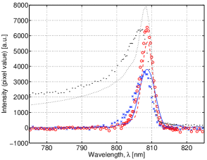
Figure 7: Color online. Spectrogram of signal emission inside single-mode fibers without interference filters. The crosses ($\Delta\lambda_{\text{s}}=6$ nm) and circles ($\Delta\lambda_{\text{s}}=4$ nm) represent experimental data for the H and the V crystal, respectively, to be compared to theoretical predictions for a 2 nm (solid line) and a 3 nm (dashed line) long crystal. Also shown is the downconversion spectrum in free space, experimentally (dots) and in theory (dotted line), demonstrating the fiber’s own filtering.

The bandwidth was found to be 4 nm for the V-crystal and 6 nm for the H-crystal. The results in Ljunggren and Tengner (2005) suggests that the effective lengths of the crystals being poled must then be 3 mm and 2 mm, respectively, but also that the 2 mm crystal should give $\approx 55\%$ of the photon-rate of the 3 mm one. Experimental agreement is good, as we saw the H-crystal giving half the rate of the V-crystal. When measuring, we refocused the fiber coupling for each crystal to find maximum counts, while keeping the pump polarization exactly at $45^{\circ}$. As described in connection to Fig. 2, the best tradeoff when collecting from both crystals simultaneously is to set the focus of the pump mode and the fiber-matched modes at the intersecting faces. Experimentally, however, in order to produce as pure a Bell-state as possible, we needed to balance the rate of each crystal, which we did by shifting the fiber-matched focus a bit closer to the H-crystal and by turning the pump-polarization slightly towards H. (The focus point was moved by turning the focusing knob on the fiber coupler.) In this way we allowed lower coupling efficiencies than the maximum attainable. The focusing conditions achieved with available lenses were, $\xi_{\text{p}}=2.1$ for the pump mode, $\xi_{\text{s}}=3.2$ for the signal’s fiber-matched mode, and $\xi_{\text{i}}=2.5$ for the idler’s.

With this configuration, we obtained the results showed in Table 1. In each column of the table, $\gamma_{\text{s}}$ represents the signal’s single coupling efficiency, $\gamma_{\text{i}}$ the idler’s, $\gamma_{c}$ the pair coupling efficiency, $\mu_{\text{i}|\text{s}}$ the conditional coincidence, and $\sigma$ the correlation efficiency, which corresponds directly to $\mu_{\text{i}|\text{s}}$ but includes a compensation for the $35\%$ transmission of the 1550 nm filter and the $85\%$ transmission of the 810 nm filter. The singles photon-rate in the signal fiber, $R_{\text{s}}$, and the idler $R_{\text{i}}$, were both derived from detected raw counts. The total generated rate $R_{\text{p}}$ of pairs before fiber coupling was estimated from detected counts using a multimode fiber. The pair rate in the fibers, $R_{\text{c}}$, was deduced from the above efficiencies and the detected raw coincidence rate, with accidental counts subtracted by assuming that $R_{\text{i}}$ originates from a Poissonian distribution at random gating Tengner and Ljunggren (2005). The conversion efficiency $\beta$ is the fraction of pump photons converted into signal and idler pairs, leading to a pair production rate $R_{\text{c}}^{\text{prod}}$, which equals $5\times 10^{3}$ s^-1THz^-1mW^-1 at the pump power $P_{\text{p}}=60\ \text{mW}$ and with the idler detector gated at 585 kHz. (The production rate is the pair rate normalized to the wavelength bandwidth in THz and the pump power in mW.) The second row of Table 1 shows similar results for a lower pump power and an idler gate rate of 91 kHz. We also took measurements without any interference filter at the idler side (but still with a 2 nm filter at the signal), with the results shown in the third row of Table 1, for $P_{\text{p}}=540\ \mu\text{W}$ and with a gate-rate of 57 kHz. The results are improved, not because of the lower power, but because of a simultaneous optimization of the arms in order to maximize $\gamma_{\text{c}}$. The table shows how $\gamma_{\text{i}}$ decreases in the process. The correlation efficiency $\sigma$ now includes the estimated transmission-loss of the optics at the idler side, and a correction factor for the unequal filtering between signal and idler (the idler fiber itself provides a frequency filtering of $\Delta\lambda_{\text{i}}=14.7$ nm). The best conditional coincidence is $\mu_{\text{i}|\text{s}}=0.27$, and the conversion efficiency, $\beta=3\times 10^{-10}$, was possibly improved by aligning to a more homogeneously poled area of the crystals. We believe that the pair production rate, $55\times 10^{3}$ s^-1THz^-1mW^-1, is one of the highest yet reported for polarization entangled photon pairs generated in crystals and launched into single-mode fibers. Frequency filtering at a narrow bandwidth of 50 GHz would imply $3\times 10^{3}$ s^-1mW^-1 of pairs in the fibers. Besides, for narrow filtering, the photon flux has been shown Ljunggren and Tengner (2005) to be $\propto L\sqrt{L}$, and so, by using longer crystals ($L=50$ mm) we could still reach 20 s^-1mW^-1 at a 10 MHz bandwidth, which is the bandwidth regime of e.g. Rb-atom based quantum memories. As a comparison, we have derived numbers using data available for some other experiments, among which the best include Fiorentino et al. Fiorentino et al. (2004), who seem to have $22\times 10^{3}$ s^-1THz^-1mW^-1 of pairs being generated by two 10 mm long crystals into free-space; K nig et al. Konig et al. (2005), who claim to have $300\times 10^{3}$ s^-1THz^-1mW^-1 pairs from two 20 mm long crystals into fibers; and Li et al. Li et al. (2005b), who seem to have an exceptional value of $4.3\times 10^{6}$ s^-1THz^-1mW^-1 pairs generated directly inside a non-linear fiber.

Fig. 8 shows the visibility curves obtained, with and without subtraction of background counts, including false coincidences. Note that the number of “accidental” coincidences increases with the pump power, as the probability of more than a single pair to arrive within the gate-time of the detector increases, as shown in section II.

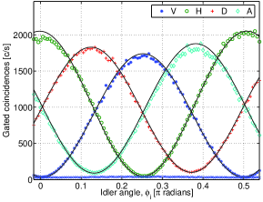
Figure 8: Color online. The plot shows the raw visibility curves obtained at a pump power $P_{\text{p}}=4.5$ mW, gate-rate 91 kHz, without subtraction of background counts (including accidentals) shown at the bottom. Each curve correspond to a different polarization setting of the signal arm, $\phi_{\text{s}}^{\text{V}}=-3\pi/16$, $\phi_{\text{s}}^{\text{H}}=\pi/16$, $\phi_{\text{s}}^{\text{D}}=-\pi/16$, and $\phi_{\text{s}}^{\text{A}}=3\pi/16$, as indicated the inset. Fitting of the collected data gives $V_{\text{H}}=99.6\pm 0.2\%$, $V_{\text{V}}=99.2\pm 0.2\%$, $V_{\text{D}}=92.7\pm 0.2\%$, and $V_{\text{A}}=94.2\pm 0.2\%$. When background counts were not subtracted, we obtained the visibilities $V_{\text{H}}=95.6\pm 0.2\%$, $V_{\text{V}}=96.2\pm 0.2\%$, $V_{\text{D}}=89.6\pm 0.2\%$, and $V_{\text{A}}=90.9\pm 0.2\%$.

We have also measured a violation of the CHSH-inequality Clauser et al. (1969) by taking measurements of the coincidence-rate functions

$$R_{i,j}=\frac{1}{2}[1+ijV_{i,j}\cos(4\phi_{\text{s}}+4\phi_{\text{i}})],$$ (19)

where $i,j=\pm 1$ denotes the four combinations of measurable output-arms of the two PBS:s in the signal and idler, $V_{i,j}$ is the corresponding visibility, and $\phi_{\text{s}}$, $\phi_{\text{i}}$, are the angles of the HWPs. The correlation function becomes

$$E(\phi_{\text{s}},\phi_{\text{i}}) =\frac{R_{1,1}-R_{1,-1}-R_{-1,1}+R_{-1,-1}}{R_{1,1}+R_{1,-1}+R_{-1,1}+R_{-1,-1}}$$

$$=V\cos(4\phi_{\text{s}}+4\phi_{\text{i}}),$$ (20)

where $V=V_{1,1}$, assuming fully equal rate functions, so that we can rely on measurements taken at only one of the output arms. Entanglement is present iff the CHSH-inequality is violated,

$$S=E(\phi_{\text{s}}^{1},\phi_{\text{i}}^{1})+E(\phi_{\text{s}}^{1},\phi_{\text{i}}^{2})+|E(\phi_{\text{s}}^{2},\phi_{\text{i}}^{1})-E(\phi_{\text{s}}^{2},\phi_{\text{i}}^{2})|\leq 2,$$ (21)

where the correlation function is to be measured at the following pair of angles: $\phi_{\text{s}}^{1}=-\pi/16,\phi_{\text{i}}^{1}=0$ and $\phi_{\text{s}}^{2}=\pi/16,\phi_{\text{i}}^{2}=\pi/8$. The parameter $S$ can reach the maximum value of $2\sqrt{2}$, corresponding to $100\%$ visibility, and it is well known that the average visibility needs to be $>71\%$ to violate the inequality, if the state is subject to equal decoherence in all bases. In our case, the state decoheres in the H/V-basis, while maintaining nearly perfect visibility for the H and V settings. Let $\phi_{\text{s}}^{1}$ represent the H/V-basis, and $\phi_{\text{s}}^{2}$ the D/A-basis. Furthermore, let $V_{\text{H},\text{V}}$ and $V_{\text{D},\text{A}}$ represent the visibilities in each respective basis. We get

$$S =V_{\text{H},\text{V}}\cos(-\frac{\pi}{4}+0)+V_{\text{H},\text{V}}\cos(-\frac{\pi}{4}+\frac{\pi}{2})+$$

$$\quad\left|V_{\text{D},\text{A}}\cos(\frac{\pi}{4}+0)-V_{\text{D},\text{A}}\cos(\frac{\pi}{4}+\frac{\pi}{2})\right|$$

$$=\sqrt{2}(V_{\text{H},\text{V}}+V_{\text{D},\text{A}}),$$ (22)

which shows that, for $V_{\text{H},\text{V}}=100\%$, the requirement is $V_{\text{D},\text{A}}>41\%$ for a violation of Eq. (21).

A direct measurement of $S$ at the above angles yields $S=2.679\pm 0.004$ at a pump power $P_{\text{p}}=60$ mW, after subtraction of accidental counts (gate-rate was 585 kHz). The CHSH-inequality was violated by 177 standard deviations in 10 s, or $56\sigma_{S}^{\phantom{1}}\ \text{s}^{-1/2}$. To our knowledge, this is one of the highest reported to date; only Kurtsiefer et al. Kurtsiefer et al. (2001a) exceeds this rate, with $148\sigma_{S}^{\phantom{1}}\ \text{s}^{-1/2}$. Other examples of good results can be found in Kwiat et al. (1999) ($50\sigma_{S}^{\phantom{1}}\ \text{s}^{-1/2}$) and in Fiorentino et al. (2004) ($38\sigma_{S}^{\phantom{1}}\ \text{s}^{-1/2}$). We have re-derived these numbers using available data, in the hopes of having created directly comparable normalized numbers. The derivation was made as follows. Assuming no fluctuation of the rate other than that originating from Poissonian-distributed single-photon detections, the standard deviation of the coincidence rate $R_{i,j}$ becomes $\sigma_{R}^{\phantom{1}}={\sqrt{R_{\text{max}}/2}}/{\sqrt{T_{R}}}$, where $R_{\text{max}}$ is the peak coincidence rate, $\sqrt{R_{\text{max}}/2}$ is the standard deviation of the average photon-rate, $T_{R}$ is the integration-time in seconds, and the central limit theorem is used to sum over time. According to Eq. (20), the standard deviation of the correlation function becomes $\sigma_{E}^{\phantom{1}}=\sqrt{4}\sigma_{R}^{\phantom{1}}/2R_{\text{max}}$, and by Eq. (21) we have $\sigma_{S}^{\phantom{1}}=\sqrt{4}\sigma_{E}^{\phantom{1}}=2/\sqrt{2R_{\text{max}}T_{R}}$, such that $S=S_{m}\pm\sigma_{S}^{\phantom{1}}$, where $S_{m}$ is the measured value over $T_{R}$ seconds. Thus, the normalized “speed of CHSH violation” becomes

$$x=\frac{S_{m}-2}{\sigma_{S}^{\phantom{1}}\sqrt{T_{R}}}=\frac{(S_{m}-2)\sqrt{2R_{\text{max}}}}{2}\quad[\text{s}^{-1/2}],$$ (23)

which only depends on the maximum rate and the measured value of $S$. If the accidental counts are not subtracted from the coincidence counts, we instead measure the value $S=2.6283\pm 0.0102$ ($P_{\text{p}}=4.5$ mW), with the CHSH-inequality being violated by $19\sigma_{S}^{\phantom{1}}\ \text{s}^{-1/2}$, showing that we truly have a high degree of entanglement launched into the fibers. This is important in entanglement-based quantum key distribution (QKD) systems that do not allow a subtraction of the background. Rather, any accidentals will increase the quantum bit error rate (QBER) and reduce the final bit rate, equivalently degrading the system performance.

Following Ref. James et al. (2001), we have made a complete tomography of the state, with the resulting density matrix becoming

$$\bm{\rho}_{\text{exp}}=\left[\begin{smallmatrix}0.5197&-0.0237&0.0300&0.4573\\ -0.0237&0.0069&0.0146&-0.0114\\ 0.0300&0.0146&0&0.0010\\ 0.4573&-0.0114&0.0010&0.4734\end{smallmatrix}\right]\\ +i\left[\begin{smallmatrix}0&0.0628&-0.0150&0.0720\\ -0.0628&0&-0.1107&0.0206\\ 0.0150&0.1107&0&-0.0581\\ -0.0720&-0.0206&0.0581&0\end{smallmatrix}\right],$$ (24)

which is also plotted in Fig. 9. Recall that the off-diagonal element, $\rho_{1122}=0.457$, corresponds approximately to the visibility in the D/A-basis, $V\approx 2\rho_{1122}=0.915$, which is indeed close to the measured visibilities. When applying the density matrix to Wootters’s entanglement of formation measure Wootters (1998), we get the value $E=0.56$. The entanglement of formation equals unity for a pure Bell-state, as do the fidelity, $F=\langle\bm{\Phi}^{\varphi}|\bm{\rho}_{\text{exp}}|\bm{\Phi}^{\varphi}\rangle$, which is found to be 0.95 for the generated state.

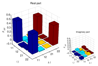
Figure 9: Color online. Experimentally determined density matrix, $\bm{\rho}_{\text{exp}}$, (real and imaginary parts) obtained by quantum state tomography on the generated polarization entangled state (1 = “V” and 2 = “H”). (Pump power, $P_{\text{p}}=4.5$ mW).

VI Future directions: A hybrid-coded entanglement source

In order to motivate the usefulness of the source, we provide in Fig. 10 a complete setup for quantum communication (e.g. QKD). The scheme, which is under implementation, uses long crystals ($2\times 50$ mm) in order to achieve a bandwidth of $<80$ GHz, which means higher production rates and less dispersion in combination with a telecom Bragg grating as dispersion compensator. For long crystals, the optimal focusing is weaker, which leads to a more compact source with fewer collimating lenses placed at closer distances to each other. Furthermore, improvement of the conditional coincidences as well as the size of the source can be achieved by minimizing the number of components, each of which contribute to loss.

In Bob’s arm, the polarization information is converted into time information in order to avoid the polarization dispersion in standard telecom fibers. (For a thorough review on photonic qubits, please refer to Tittel and Weihs (2001).) A polarizing beam splitter sits in an unbalanced Mach-Zehnder interferometer, directing vertical photons into the long arm and horizontal into the short. The vertical photons are rotated to horizontal before the photons in both arms are recombined on a fiber-based beam-splitter and sent to a Bragg grating. The result is a time encoded qubit with all polarization information erased. (To our knowledge, there is no way to erase this information passively without having to accept 50% losses in the unused arm of the beam-splitter, which is an disadvantage, but could also be turned to an advantage by introducing a third party Charlie.) The resulting state becomes $|\Phi^{\prime}\rangle=1/\sqrt{2}\left(|\text{V}\rangle_{\text{s}}|\text{L}\rangle_{\text{i}}+e^{i\varphi}|\text{H}\rangle_{\text{s}}|\text{S}\rangle_{\text{i}}\right)$, where L denotes the long arm and S the short arm.

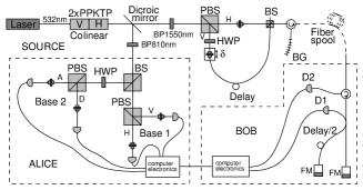
Figure 10: Scheme to create hybrid-coded entanglement. BS: beam splitter, PBS: polarizing beam splitter, HWP: half-wave plate, BP: band-pass filter, BG: Bragg grating, FM: Faraday mirror.

On Bob’s analyzer side, there is an unbalanced all-fiber Michelson interferometer with a single beam-splitter to decode the qubits. The interferometer uses Faraday mirrors, which reflect the light in such a way that the polarization is exactly orthogonal when the photons arrive a second time at the beam-splitter to interfere, and thereby avoids the need for polarization controllers Tittel et al. (1998). The phase information of the qubit defines a complementary basis to time, and for that information to remain, the path length difference between the short and the long arm needs to be exactly matched to that of the preparing interferometer, requiring both interferometers to be temperature stabilized. However, longer coherence length of the emitted photons (an effect of narrow bandwidth) will effectively relax these requirements. One advantage of the above solution is that the preparing interferometer has translatable fiber couplers inside the interferometer, which simplifies their mutual alignment. Also, we avoid the possibly difficult alignment of three interferometers, as Alice adheres to polarization coding. Another important condition for the qubits to remain coherent is that the delay between two consecutive pulses is short enough ($\approx 5$ ns) that they experience the same phase shift due to vibrations and temperature fluctuations when traveling over the fiber. On Alice’s side, the analyzer realizes a standard polarization decoder. Note that the H/V or D/A-basis is randomly chosen by the first beam-splitter, just as at Bob’s side, which implies that there is no need for any active devices. Note also that there exists the possibility to delay the outputs of each detector arm on Alice side and combine into different time-slots for detection with a single detector, instead of four, which may reduce the need for space.

VII Summary

In this article, we have presented work on a two-crystal source that uses PPKTP for the production of polarization-entangled photon-pairs in a single spatial mode, leading to efficient fiber coupling. The source is suitable for schemes that combine polarization and time coding. We have shown how distinguishability between photon-pairs is introduced for this type of colinear source, due to a special kind of chromatic two-photon dispersion. We have derived and analyzed the output state of SPDC for this case, with the goal to cancel the decoherence and regain a pure state using an extra piece of birefringent crystal. We have determined the quality of entanglement for the reported setup using various measures, including the method of quantum state tomography, and we draw the conclusion that this is one of the brightest sources available for polarization entanglement in terms of Bell-inequality violation and production rates.

*

Appendix A The two-photon frequency and polarization quantum state

In this Appendix, we derive the quantum state of a single crystal in terms of frequency and polarization degrees of freedom, using the interaction picture of SPDC Klyshko (1988).

The evolution of the number state vector is given by

$$|\psi\rangle =\exp\left[\frac{1}{i\hbar}\int\limits_{T}^{t_{0}+T}\!\!\text{d}t\hat{H}(t)\right]|\psi_{00}\rangle$$

$$\approx\left(\openone+\frac{1}{i\hbar}\int\limits_{T}^{t_{0}+T}\!\!\text{d}t\hat{H}(t)\right)|\psi_{00}\rangle,$$ (25)

where $|\psi_{00}\rangle$ is the number state at time $t_{0}$ and $\hat{H}(t)$ is the interaction Hamiltonian,

$$\hat{H}(t)=\int\limits_{-L/2}^{L/2}\!\!\!\!\text{d}z\!\!\int\limits_{-\infty}^{\infty}\!\!\!\text{d}y\!\!\int\limits_{-\infty}^{\infty}\!\!\!\text{d}x\>\chi^{(2)}\hat{E}_{\text{p}}^{(+)}\hat{E}_{\text{s}}^{(-)}\hat{E}_{\text{i}}^{(-)}+\mathrm{H.c.},$$ (26)

displayed in a Cartesian coordinate system, $\bm{r}=x\bm{e}_{x}+y\bm{e}_{y}+z\bm{e}_{z}$. There are three interacting fields in the crystal’s volume, ignoring all higher-order terms ($n\geq 3$) of the non-linearity $\chi^{(n)}$. All three fields have the same polarization ($ZZZ$):

$$E_{\text{p}}^{(+)}=E_{0}\>e^{-i(k_{0\text{p}}\bm{s}_{\text{p}}\cdot\bm{r}-\omega_{\text{p}}t+\phi_{\text{p}})}$$ (27)

$$\hat{E}_{\text{s}}^{(-)}=\!\int\!\!\text{d}\phi_{\text{s}}\int\!\!\text{d}\omega_{\text{s}}A_{\text{s}}(\omega_{\text{s}})\sum\limits_{\bm{s}_{\text{s}}}e^{i(k_{\text{s}}\bm{s}_{\text{s}}\cdot\bm{r}-\omega_{\text{s}}t+\phi_{\text{s}})}\hat{a}_{\text{s}}^{\dagger}(\omega_{\text{s}},\bm{s}_{\text{s}})\!\!\!$$ (28)

$$\hat{E}_{\text{i}}^{(-)}=\!\int\!\!\text{d}\phi_{\text{i}}\int\!\!\text{d}\omega_{\text{i}}A_{\text{i}}(\omega_{\text{i}})\sum\limits_{\bm{s}_{\text{i}}}e^{i(k_{\text{i}}\bm{s}_{\text{i}}\cdot\bm{r}-\omega_{\text{i}}t+\phi_{\text{i}})}\hat{a}_{\text{i}}^{\dagger}(\omega_{\text{i}},\bm{s}_{\text{i}}),$$ (29)

where the pump field is classical and monochromatic so that we can replace $\hat{E}_{\text{p}}^{(+)}$ by $E_{\text{p}}^{(+)}$. The plus sign denotes conjugation, i.e annihilation (+) or creation (-) of the state. We have also introduced the notation $\bm{k}=k\bm{s}$, where $\bm{s}=p\bm{e}_{x}+q\bm{e}_{y}+m\bm{e}_{z}$, is the unit length vector of $\bm{k}$ with components in each of the three dimensions Mandel and Wolf (1995), as defined by the coordinate system in Fig. 1. The pump field is a plane wave propagating in the $z$-direction, $\bm{s}_{\text{p}}=\bm{e}_{z}$. For signal and idler, we sum over both frequency and angular modes, where $\hat{a}(\omega,\bm{s})$ is the field operator, and $A(\omega)$ is the frequency amplitude of a Gaussian-shaped detector filter having the bandwidth $\Delta\lambda$ (FWHM) and center wavelength $\lambda_{c}^{\phantom{1}}$ (all wavelengths in vacuum). Via the relation $\omega=2\pi cn_{\!\scriptscriptstyle\lambda}/\lambda$, its form is given by

$$A(\omega;\lambda)=e^{-2\log(2)(\lambda-\lambda_{c}^{\phantom{1}})^{2}/\Delta\lambda^{2}}.$$ (30)

Each signal and idler photon is created with a random phase, $\phi_{\text{s}}$ and $\phi_{\text{i}}$, respectively, which we need to sum over. The phase of the pump, $\phi_{\text{p}}$, is constant and arbitrary.

For periodically poled materials, the spatial variation of the nonlinear index $\chi^{(2)}$ has sharp boundaries, but we will simplify and make a sinusoidal approximation using the first term of an Fourier-series expansion of $\chi^{(2)}$:

$$\chi^{(2)}=\chi_{2}^{\phantom{1}}\sum_{m=0}^{\infty}f_{m}e^{-im\bm{K}\cdot\bm{r}}\approx\chi_{2}^{\phantom{1}}\>f_{1}e^{-i\bm{K}\cdot\bm{r}},$$ (31)

where $\bm{K}=K\bm{e}_{z}={2\pi/\Lambda}\>\bm{e}_{z}$ and $\Lambda$ is the grating period.

The Hamiltonian now takes the form

$$\hat{H}(t) =\chi_{2}^{\phantom{1}}\>f_{1}E_{0}\int\!\!\text{d}\phi_{\text{s}}\int\!\!\text{d}\phi_{\text{i}}\int\!\!\text{d}\omega_{\text{s}}\int\!\!\text{d}\omega_{\text{i}}\>$$

$$\quad\times\>A_{\text{s}}(\omega_{\text{s}})A_{\text{i}}(\omega_{\text{i}})$$

$$\quad\times\>\sum\limits_{\bm{s}_{\text{s}}}\sum\limits_{\bm{s}_{\text{i}}}\hat{a}_{\text{s}}^{\dagger}(\omega_{\text{s}},\bm{s}_{\text{s}})\hat{a}_{\text{i}}^{\dagger}(\omega_{\text{i}},\bm{s}_{\text{i}})$$

$$\quad\times\>\int\limits_{-L/2}^{L/2}\!\!\!\!\text{d}z\!\!\int\limits_{-\infty}^{\infty}\!\!\!\text{d}y\!\!\int\limits_{-\infty}^{\infty}\!\!\!\text{d}x$$

$$\quad\times\>e^{-i[\Delta\bm{k}\cdot(x\bm{e}_{x}+y\bm{e}_{y}+z\bm{e}_{z})\>-\>(\omega_{\text{s}}+\omega_{\text{i}}-\omega_{\text{p}})t\>+\>\phi_{\text{s}}+\phi_{\text{i}}-\phi_{\text{p}}]}$$

$$\quad+\>\mathrm{H.c.},$$ (32)

where the mismatch vector is

$$\Delta\bm{k} =k_{\text{s}}\bm{s}_{\text{s}}+k_{\text{i}}\bm{s}_{\text{i}}-k_{0\text{p}}\bm{s}_{\text{p}}+\bm{K}$$

$$=\Delta k_{x}\bm{e}_{x}+\Delta k_{y}\bm{e}_{y}+\Delta k_{z}\bm{e}_{z}.$$ (33)

Following Eq. (25), we now let the Hamiltonian undergo time evolution. The mismatch vector is also divided up into its x, y, and z components using Eq. (33). Hence,

$\displaystyle\frac{1}{i\hbar}\int\!\!\text{d}t\hat{H}(t)=$

$$\quad\chi_{2}^{\phantom{1}}\>f_{1}E_{0}\int\!\!\text{d}\omega_{\text{s}}\int\!\!\text{d}\omega_{\text{i}}\>A_{\text{s}}(\omega_{\text{s}})A_{\text{i}}(\omega_{\text{i}})$$

$$\quad\times\>\sum\limits_{\bm{s}_{\text{s}}}\sum\limits_{\bm{s}_{\text{i}}}\hat{a}_{\text{s}}^{\dagger}(\omega_{\text{s}},\bm{s}_{\text{s}})\hat{a}_{\text{i}}^{\dagger}(\omega_{\text{i}},\bm{s}_{\text{i}})$$

$$\quad\times\>\int\limits_{-L/2}^{L/2}\!\!\!\!\text{d}z\!\!\int\limits_{-\infty}^{\infty}\!\!\!\text{d}y\!\!\int\limits_{-\infty}^{\infty}\!\!\!\text{d}x\>e^{-i[\Delta k_{x}x+\Delta k_{y}y+\Delta k_{z}z]}\>$$

$$\quad\times\>\frac{1}{i\hbar}\iint\limits_{0}^{\quad 2\pi}\!\text{d}\phi_{\text{s}}\text{d}\phi_{\text{i}}\int\limits_{0}^{T}\!\text{d}t\>e^{-i[(\omega_{\text{s}}+\omega_{\text{i}}-\omega_{\text{p}})t\>+\>\phi_{\text{s}}+\phi_{\text{i}}-\phi_{\text{p}}]}$$

$$\quad-\>\mathrm{H.c.}.$$ (34)

The integration over the interaction volume, $\text{d}x$, $\text{d}y$, and $\text{d}z$, can now be easily carried out. There are three spatial integrals, of which two are the Fourier transforms of unity ($\text{d}x$ and $\text{d}y$) and one is the transform of a box function ($\text{d}z$). The transforms turn into two $\delta$ functions and a sinc function, respectively. The time integral also turns into a $\delta$ function of the three frequencies $\omega_{\text{s}}$, $\omega_{\text{i}}$, and $\omega_{\text{p}}$. This is because we assume a monochromatic pump beam with infinite coherence length, which effectively leads to an infinite interaction time, ${T\rightarrow\infty}$, even for short crystals. Motivated by the rotational symmetry of the emitted modes, we also change to a spherical coordinate system (see Fig. 1), by replacing the summation over $\bm{s}$ with integrals over $\theta_{\text{s}},\theta_{\text{i}},\varphi_{\text{s}}$ and $\varphi_{\text{i}}$. Furthermore, the only non-zero solution for the integration over the random phases, $\phi_{\text{s}}$ and $\phi_{\text{i}}$, is for the phases to add up to a constant, yielding the relation ${\phi_{\text{s}}+\phi_{\text{i}}=\phi_{\text{p}}+C}$. If we let $C=0$ for simplicity, and drop some constants resulting from the integrations, we are led to

$$\frac{1}{i\hbar}\int\!\!\text{d}t\hat{H}(t) =\frac{1}{i\hbar}\chi_{2}^{\phantom{1}}\>f_{1}E_{0}\int\!\!\text{d}\omega_{\text{s}}\int\!\!\text{d}\omega_{\text{i}}\>A_{\text{s}}(\omega_{\text{s}})A_{\text{i}}(\omega_{\text{i}})$$

$$\quad\times\>\int\limits_{0}^{\pi/2}\!\!\sin\theta_{\text{s}}\>\text{d}\theta_{\text{s}}\int\limits_{0}^{\pi/2}\!\!\sin\theta_{\text{i}}\>\text{d}\theta_{\text{i}}\int\limits_{0}^{2\pi}\!\!\text{d}\varphi_{\text{s}}\int\limits_{0}^{2\pi}\!\!\text{d}\varphi_{\text{i}}\>$$

$$\quad\times\>\hat{a}_{\text{s}}^{\dagger}(\omega_{\text{s}},\theta_{\text{s}},\varphi_{\text{s}})\>\hat{a}_{\text{i}}^{\dagger}(\omega_{\text{i}},\theta_{\text{i}},\varphi_{\text{i}})\>\delta(\omega_{\text{s}}+\omega_{\text{i}}-\omega_{\text{p}})$$

$$\quad\times\>\delta(\Delta k_{x})\>\delta(\Delta k_{y})\>L\>\text{sinc}\left[\frac{L}{2}\Delta k_{z}\right]$$

$$\quad-\>\mathrm{H.c.}.$$ (35)

At this stage, we observe that $k_{\text{s}}$ and $k_{\text{i}}$ each depend on $\omega_{\text{s}}$ and $\omega_{\text{i}}$, respectively. Motivated by the $\delta$-function in Eq. (35), we let $\omega_{\text{s}}=\omega_{0\text{s}}+\epsilon$ and $\omega_{\text{i}}=\omega_{0\text{i}}-\epsilon$, and make a series expansion of the k-vectors:

$$k_{\text{s}} \approx k_{0\text{s}}+\epsilon\frac{\text{d}k_{0\text{s}}}{\text{d}\omega_{0\text{s}}}=k_{0\text{s}}+\epsilon\frac{1}{v_{\text{g},\text{s}}^{Z}}=k_{0\text{s}}+\epsilon\frac{n_{\text{g},\text{s}}^{Z}}{c}$$ (36a)

$$k_{\text{i}} \approx k_{0\text{i}}-\epsilon\frac{\text{d}k_{0\text{i}}}{\text{d}\omega_{0\text{i}}}=k_{0\text{i}}-\epsilon\frac{1}{v_{\text{g},\text{i}}^{Z}}=k_{0\text{i}}-\epsilon\frac{n_{\text{g},\text{i}}^{Z}}{c}.$$ (36b)

In a spherical coordinate system, we have $p=\sin\theta\cos\varphi$, $q=\sin\theta\sin\varphi$, and $m=\cos\theta$, and so the phase-mismatch vector components become

$$\Delta k_{x} =k_{\text{s}}\sin\theta_{\text{s}}\cos\varphi_{\text{s}}+k_{\text{i}}\sin\theta_{\text{i}}\cos\varphi_{\text{i}}\approx 0,$$

$$\Delta k_{y} =k_{\text{s}}\sin\theta_{\text{s}}\sin\varphi_{\text{s}}+k_{\text{i}}\sin\theta_{\text{i}}\sin\varphi_{\text{i}}\approx 0,$$

$$\Delta k_{z} =k_{\text{s}}\cos\theta_{\text{s}}+k_{\text{i}}\cos\theta_{\text{i}}-k_{0\text{p}}+K$$

$$\approx\frac{\epsilon}{c}(n_{\text{g},\text{s}}^{Z}-n_{\text{g},\text{i}}^{Z}),$$ (37)

where we have done a first-order approximation of $\sin\theta$ and $\cos\theta$ for small angles, meaning that we consider only plane waves, and where the last component is simplified using the phase-matching condition for the forward direction, $k_{0\text{s}}+k_{0\text{i}}-k_{0\text{p}}+K=0$, together with Eq. (36). Thanks to Eq. (37), we can now trivially perform the integration over the spatial modes $\text{d}\theta_{\text{s}},\text{d}\theta_{\text{i}}$ and $\text{d}\varphi$, which finally leads to the following compact expression

$$\frac{1}{i\hbar}\int\!\!\text{d}t\hat{H}(t) =\frac{1}{i\hbar}\chi_{2}^{\phantom{1}}\>f_{1}E_{0}$$

$$\quad\times\>\int\!\!\text{d}\epsilon\>A_{\text{s}}(\epsilon)A_{\text{i}}(\epsilon)\hat{a}_{\text{s}}^{\dagger}(\epsilon)\hat{a}_{\text{i}}^{\dagger}(\epsilon)$$

$$\quad\times\>L\>\text{sinc}\left[\frac{L\epsilon}{2c}(n_{\text{g},\text{s}}^{Z}-n_{\text{g},\text{i}}^{Z})\right]$$

$$\quad-\>\mathrm{H.c.}$$

$$=\int\!\!\text{d}\epsilon\>U(\epsilon)\>\hat{a}_{\text{s}}^{\dagger}(\epsilon)\hat{a}_{\text{i}}^{\dagger}(\epsilon)\>-\>\mathrm{H.c.}.$$ (38)

In summary, Eq. (25), via Eq. (38), has helped us find the frequency and polarization state generated in one crystal, which we will write in the form

$$|\Psi_{ZZ}\rangle =\frac{1}{B}\int\!\!\text{d}\epsilon\>U(\epsilon)\>|\bm{\epsilon}\rangle\otimes|\bm{\chi}_{ZZ}^{\phantom{1}}\rangle,$$ (39)

where $U(\epsilon)$ is defined by Eq. (38), and where

$$B =\frac{\left(\int\!\text{d}\epsilon|A_{\text{s}}(\epsilon)A_{\text{i}}(\epsilon)|^{2}\>\text{sinc}^{2}[L\epsilon(n_{\text{g},\text{s}}^{Z}-n_{\text{g},\text{i}}^{Z})/2c]\right)^{1/2}}{\hbar(\chi_{2}^{\phantom{1}}\>f_{1}E_{0}L)^{-1}_{\phantom{1}}},$$ (40)

is a normalization constant, such that $|\frac{1}{B}\int\!\text{d}\epsilon\>U(\epsilon)|^{2}=1$. Here, $\bm{\epsilon}$ represents the frequency mode and $\bm{\chi}_{ZZ}^{\phantom{1}}$ represents the polarization mode along the $Z$-axis.

References

- Kwiat et al. (1995) P. G. Kwiat, K. Mattle, H. Weinfurter, A. Zeilinger, A. V. Sergienko, and Y. Shih, Phys. Rev. Lett. 75, 4337 (1995).
- Jennewein et al. (2000) T. Jennewein, C. Simon, G. Weihs, H. Weinfurter, and A. Zeilinger, Phys. Rev. Lett. 84, 4729 (2000).
- Kurtsiefer et al. (2001a) C. Kurtsiefer, M. Oberparleiter, and H. Weinfurter, Phys. Rev. A 64, 023802 (2001a).
- Kiess et al. (1993) T. E. Kiess, Y. H. Shih, A. V. Sergienko, and C. O. Alley, Phys. Rev. Lett. 71, 3893 (1993).
- Tittel et al. (1999) W. Tittel, J. Brendel, N. Gisin, and H. Zbinden, Phys. Rev. A 59, 4150 (1999).
- Kim et al. (2000) Y. H. Kim, S. P. Kulik, and Y. Shih, Phys. Rev. A 62, 011802(R) (2000).
- Takesue and Inoue (2004) H. Takesue and K. Inoue, Phys. Rev. A 70, 031802(R) (2004).
- Li et al. (2005a) X. Li, P. L. Voss, J. Chen, J. E. Sharping, and P. Kumar, Opt. Lett. 30, 1201 (2005a).
- Li et al. (2005b) X. Li, P. L. Voss, J. E. Sharping, and P. Kumar, Phys. Rev. Lett. 94, 053601 (2005b).
- Hardy (1992) L. Hardy, Phys. Lett. A 161, 326 (1992).
- Kwiat et al. (1999) P. G. Kwiat, E. Waks, A. G. White, I. Appelbaum, and P. H. Eberhard, Phys. Rev. A 60, R773 (1999).
- Fiorentino et al. (2004) M. Fiorentino, G. Messin, C. E. Kuklewicz, F. N. C. Wong, and J. Shapiro, 69, 041801 (2004).
- Mason et al. (2002) E. J. Mason, M. A. Albota, F. Knig, and F. N. C. Wong, Opt. Lett. 27, 2115 (2002).
- Tanzilli et al. (2002) S. Tanzilli, W. Tittel, H. D. Riedmatten, H. Zbinden, P. Baldi, M. D. Micheli, D. Ostrowsky, and N. Gisin, Eur. Phys. J. D 18, 155 (2002).
- Ljunggren and Tengner (2005) D. Ljunggren and M. Tengner (2005), eprint arXiv.org:quant-ph/0507046.
- Halder et al. (2005) M. Halder, S. Tanzilli, H. de Riedmatten, A. Beveratos, H. Zbinden, and N. Gisin, Phys. Rev. A 71, 042335 (2005).
- Ekert (1991) A. K. Ekert, Phys. Rev. Lett. 67, 661 (1991).
- Pelton et al. (2004) M. Pelton, P. Marsden, D. Ljunggren, M. Tengner, A. Karlsson, A. Fragemann, C. Canalias, and F. Laurell, Opt. Express. 12, 3573 (2004).
- Tanzilli et al. (2005) S. Tanzilli, W. Tittel, M. Halder, O. Alibart, P. Baldi, N. Gisin, and H. Zbinden, Nature 437, 116 (2005).
- Konig et al. (2005) F. Konig, E. J. Mason, F. N. C. Wong, and M. A. Albota, Phys. Rev. A 71, 033805 (2005).
- Ribordy et al. (2000) G. Ribordy, J. Brendel, J. D. Gauthier, N. Gisin, and H. Zbinden, Phys. Rev. A 63, 012309 (2000).
- Tittel et al. (2000) W. Tittel, J. Brendel, H. Zbinden, and N. Gisin, Phys. Rev. Lett. 84, 4737 (2000).
- Fan et al. (1987) T. Y. Fan, C. E. Huang, B. Q. Hu, R. C. Eckardt, Y. X. Fan, R. L. Byer, and R. S. Feigelson, Appl. Opt. 26, 2390 (1987).
- Fradkin et al. (1999) K. Fradkin, A. Arie, A. Skliar, and G. Rosenman, Appl. Phys. Lett. 74, 914 (1999).
- Tengner and Ljunggren (2005) M. Tengner and D. Ljunggren, in preparation (2005).
- Kuklewicz et al. (2004) C. E. Kuklewicz, M. Fiorentino, G. Messin, F. N. C. Wong, and J. H. Shapiro, Phys. Rev. A 69, 013807 (2004).
- Clauser et al. (1969) J. F. Clauser, M. A. Horne, A. Shimony, and R. A. Holt, Phys. Rev. Lett. 23, 880 (1969).
- James et al. (2001) D. F. V. James, P. G. Kwiat, W. J. Munro, and A. G. White, Phys. Rev. A 64, 052312 (2001).
- Wootters (1998) W. K. Wootters, Phys. Rev. Lett. 80, 2245 (1998).
- Tittel and Weihs (2001) W. Tittel and G. Weihs, Quant. Inf. Comput. 1, 3 (2001), eprint arXiv.org:quant-ph/0107156.
- Tittel et al. (1998) W. Tittel, J. Brendel, H. Zbinden, and N. Gisin, Phys. Rev. Lett. 81, 3563 (1998).
- Klyshko (1988) D. N. Klyshko, Photons and Nonlinear Optics (Gordon and Breach Science Publishers, New York, 1988).
- Mandel and Wolf (1995) L. Mandel and E. Wolf, Optical Coherence and Quantum Optics (Cambridge University Press, 1995).