The classical capacity for the quantum Markov channel of continuous variables

Abstract

Quantum communications using continuous variables are quite mature experimental techniques and the relevant theories have been extensively investigated with various methods. In this paper, we study the continuous variable quantum channels from a different angle, i.e., by exploring master equations. And we finally give explicitly the capacity of the channel we are studying. By the end of this paper, we derive the criterion for the optimal capacities of the Gaussian channel versus its fidelity.

I Introduction

The evaluation of information capacities of quantum channels is one of the most challenging and intractable questions of quantum information theory chuang . Previous research primarily focuses on discrete input alphabet. However, quantum information transmission with continuous alphabet is an interesting alternative to the classical discrete alphabet based approach pati ; cover . Many efforts have been devoted to characterize continuous alphabet quantum channels bennett . It is also important to investigate the capacity of the continuous-variable quantum channels acting on a bosonic field. Such issue has been addressed recently holevo1 ; giovannetti ; macchiavello . All these intriguing works mentioned above have brought significant progress in the studies of continuous-variable quantum channels.

One rationale is that any quantum operation is a completely positive trace-preserving map(CPT) and therefore it can be considered as a quantum channel. On the other hand, when the physical system of interest interacts with the environment, irreversible decoherence can occur, causing the pure states to become mixed states zurek ; joos . This process depicts the influence of noise over quantum states, which can be envisioned as transmission of information under noisy circumstances. Sonja et al. have investigated these kinds of noisy quantum channels for qubits, which they call the squeezed vacuum channel, by making use of the master equation sonja . These studies provide a unique angle to address this issue. However, their work is restricted to noisy quantum channels acting on finite-dimensional Hilbert space, while the studies on continuous variable system by using the master equation are obscure.

In this paper, we investigate the master equation of the decaying monomodal electromagnetic field interacting with the thermal reservoir. We consider the evolution of the density operator as a kind of information transmission process undergoing a noisy quantum Markov channel. The channel we study is Markovian, so memory is not an issue here markov .

In the article we will give explicitly the capacity of the Markov channel. The material is organized as follows. We begin this paper by introducing the quantum Markov channel and its general properties in the first part of Sec. II. The explicit solution to the master equation is discussed in the second part of Sec. II. In the third part of Sec. II, we give detailed calculation of the capacity of the quantum Markov channel. In Sec. III, some discussions are made. The capacity result is analyzed. In Sec. IV, we will discuss the fidelity of the channel transmission and derive for the particular input signal such that the channel capacity and channel fidelity are mutually optimal. And in Sec. V, we will arrive at the final conclusions.

II Quantum Markov channels

II.1 General properties of the Markov channel

Generally speaking, any quantum physical operation that reflects the time evolution of a quantum state can be regarded as a quantum channel. Precisely, the basic concept of quantum information theory is that the message is encoded in certain quantum states, which are transmitted through some quantum channel, then the receiver decodes the quantum states at his hand to retrieve the information.  As a CPT, certainly the master equation does reflect the time evolution of a density operator. Thereupon the master equation defines a channel $\$$

$$\$:\rho\rightarrow\$\left(\rho\right)$$

Master equations intrinsically describe evolutions local in time, namely, Markovian processes preskill . Therefore, the quantum channels that master equations define are quantum Markov channels.

According to Holevo-Schumacher-Westmoreland (HSW) theorem holevo2 , the one-shot classical capacity of the quantum channel $\$$ is defined

$$\chi\left(\$\right)\equiv\max_{\left\{p_{i},\rho_{i}\right\}}\left[S\left(\$\left(\sum_{i}p_{i}\rho_{i}\right)\right)-\sum_{i}p_{i}S\left(\$\left(\rho_{i}\right)\right)\right]$$ (1)

where the maximum is over all ensembles $\left\{p_{i},\rho_{i}\right\}$ of possible input states $\rho_{i}$ to the channel. Here $S\left(\rho\right)=-Tr\left[\rho\log\rho\right]$ is the von Neumann entropy. We declare here that the basis of the logarithm function is 2 all through the paper. In this case, $\chi\left(\$\right)$ is in units of bit. The procedure to calculate the channel capacity requires a maximization over all the input states. So far as the continuous-variable quantum channel is concerned, it is conjectured that a Gaussian mixture of coherent states, namely, thermal state, achieves the Gaussian channel capacity $\chi\left(\$\right)$ macchiavello .

II.2 The master equation and its solution

Here we consider the case that monomodal electromagnetic field interacting with the thermal reservoir, i.e., the damping harmonic oscillators coupled to the squeezed thermal reservoir. The interaction Hamiltonian of the system is scully

$$H=\hbar\sum_{k}g_{k}\left[b_{k}^{+}ae^{-i(\nu-\nu_{k})t}+a^{+}b_{k}e^{i(\nu-\nu_{k})t}\right]$$

where $a$ (and $a^{+}$) are the annihilation (and creation) operators of the mode of interest. The operators $b_{k}^{+}$ and $b_{k}$ represent modes of the reservoir that damp the field. When the modes $b_{k}$ are initially in a squeezed vacuum, the evolution of the reduced density operator in the interaction picture is described by the master equation given below scully ; milburn

$$\frac{d\rho}{dt} = \frac{\gamma}{2}(N+1)(2a\rho a^{+}-a^{+}a\rho-\rho a^{+}a)$$

$$+\frac{\gamma}{2}N(2a^{+}\rho a-aa^{+}\rho-\rho aa^{+})$$

$$+\frac{\gamma}{2}M\left(2a^{+}\rho a^{+}-a^{+}a^{+}\rho-\rho a^{+}a^{+}\right)$$

$$+\frac{\gamma}{2}M^{\ast}\left(2a\rho a-aa\rho-\rho aa\right)$$

where $\gamma$ is the decaying rate, $N$ is the mean photon number of the reservoir, and $M$ is the parameter somehow related to the squeezed vacuum reservoir, respectivly.

The authors in lu provide the explicit solution to the master equation above. Assume the initial state is squeezed coherent state, namely,

$$\rho\left(0\right)=S\left(\zeta\right)\left|\eta\right\rangle\left\langle\eta\right|S^{+}\left(\zeta\right)$$

here $\left|\eta\right\rangle\left\langle\eta\right|$ is coherent state, and $S\left(\zeta\right)$ is squeeze operator. Therefore the final form of the output density operator is

$$\rho\left(t\right)=S\left(\zeta\right)\frac{\exp\left[-\beta\left(t\right)\left|\widetilde{\eta}\left(t\right)\right|^{2}\right]}{1+\beta\left(t\right)}\times\mathop{\displaystyle\sum}\limits_{n=0}^{\infty}\left(\frac{\beta\left(t\right)}{1+\beta\left(t\right)}\right)^{n}\frac{\left(a^{+}\right)^{n}}{n!}\left|\widetilde{\eta}\left(t\right)\right\rangle\left\langle\widetilde{\eta}\left(t\right)\right|a^{n}S^{+}\left(\zeta\right)$$

here

$$\beta\left(t\right)=\frac{\beta}{\gamma}\left(1-e^{-\gamma t}\right)$$ (3)

$$\widetilde{\eta}\left(t\right)=\frac{\eta e^{-\frac{\gamma}{2}t}}{1+\beta\left(t\right)}\equiv\eta f,f=\frac{e^{-\frac{\gamma}{2}t}}{1+\beta\left(t\right)}$$ (4)

where $\beta$ is a real number.

A unitary operator doesn’t affect classical capacity of the quantum channel, so we set $\zeta=0$. Hence the final solution has the form

$$\rho\left(t\right) = \frac{\exp\left[-\beta\left(t\right)\left|\widetilde{\eta}\left(t\right)\right|^{2}\right]}{1+\beta\left(t\right)}$$

$$\times\mathop{\displaystyle\sum}\limits_{n=0}^{\infty}\left(\frac{\beta\left(t\right)}{1+\beta\left(t\right)}\right)^{n}\frac{\left(a^{+}\right)^{n}}{n!}\left|\widetilde{\eta}\left(t\right)\right\rangle\left\langle\widetilde{\eta}\left(t\right)\right|a^{n}$$

$$= \frac{1}{1+\beta\left(t\right)}e^{-\left(1+\beta\left(t\right)\right)f^{2}\left|\eta\right|^{2}}e^{f\eta a^{+}}:e^{\frac{\beta\left(t\right)}{1+\beta\left(t\right)}a^{+}a-a^{+}a}:e^{f^{\ast}\eta^{\ast}a}$$

$$= \frac{1}{1+\beta\left(t\right)}e^{-\left(1+\beta\left(t\right)\right)f^{2}\left|\eta\right|^{2}}:e^{-\frac{1}{1+\beta\left(t\right)}a^{+}a+f\eta a^{+}+f^{\ast}\eta^{\ast}a}:$$

II.3 The channel capacity

Below we directly compute the channel capacity. Note that

$$\rho\left(t\right) = \frac{1}{1+\beta\left(t\right)}e^{-\left(1+\beta\left(t\right)\right)f^{2}\left|\eta\right|^{2}}e^{f\eta a^{+}}:e^{\frac{\beta\left(t\right)}{1+\beta\left(t\right)}a^{+}a-a^{+}a}:e^{f^{\ast}\eta^{\ast}a}$$

$$= \frac{1}{\beta\left(t\right)}e^{-\left(1+\beta\left(t\right)\right)f^{2}\left|\eta\right|^{2}}e^{f\eta a^{+}}:\int d^{2}\alpha e^{-\frac{1+\beta\left(t\right)}{\beta\left(t\right)}\left|\alpha\right|^{2}+\alpha a^{+}+\alpha^{\ast}a-a^{+}a}:e^{f^{\ast}\eta^{\ast}a}$$

$$= \frac{1}{\beta\left(t\right)}e^{-\left(1+\beta\left(t\right)\right)f^{2}\left|\eta\right|^{2}}e^{f\eta a^{+}}\int d^{2}\alpha e^{-\frac{\left|\alpha\right|^{2}}{\beta\left(t\right)}}\left|\alpha\right\rangle\left\langle\alpha\right|e^{f^{\ast}\eta^{\ast}a}$$

$$= \frac{1}{\beta\left(t\right)}\int d^{2}\alpha e^{-\frac{\left|\alpha-\beta\left(t\right)f\eta\right|^{2}}{\beta\left(t\right)}}D\left(\alpha\right)\left|f\eta\right\rangle\left\langle f\eta\right|D^{+}\left(\alpha\right)$$

With this simplification, we can see $\rho\left(t\right)$ is Gaussian. Therefore we can safely arrive at the conclusion that the channel is a Gaussian one.

Now we calculate the von Neumann entropy of $\rho\left(t\right)$. $\rho\left(t\right)$ can be transformed into

$$\rho\left(t\right) = \frac{1}{1+\beta\left(t\right)}e^{-\left(1+\beta\left(t\right)\right)f^{2}\left|\eta\right|^{2}}:e^{-\frac{1}{1+\beta\left(t\right)}a^{+}a+f\eta a^{+}+f^{\ast}\eta^{\ast}a}:$$

$$= \frac{1}{1+\beta\left(t\right)}:e^{-\frac{1}{1+\beta\left(t\right)}\left[a^{+}-\left(1+\beta\left(t\right)\right)f^{\ast}\eta^{\ast}\right]\left[a-\left(1+\beta\left(t\right)\right)f\eta\right]}:$$

$$= \frac{1}{1+\beta\left(t\right)}D\left(-e^{-\frac{\gamma}{2}t}\eta^{\ast}\right):e^{-\frac{1}{1+\beta\left(t\right)}a^{+}a}:D^{+}\left(-e^{-\frac{\gamma}{2}t}\eta^{\ast}\right)$$

$$= \frac{1}{1+\beta\left(t\right)}D\left(-e^{-\frac{\gamma}{2}t}\eta^{\ast}\right)e^{\ln\frac{\beta\left(t\right)}{1+\beta\left(t\right)}a^{+}a}D^{+}\left(-e^{-\frac{\gamma}{2}t}\eta^{\ast}\right)$$

$$= \frac{1}{1+\beta\left(t\right)}e^{\ln\frac{\beta\left(t\right)}{1+\beta\left(t\right)}\left(a^{+}-e^{\frac{\gamma}{2}t}\eta^{\ast}\right)\left(a-e^{\frac{\gamma}{2}t}\eta\right)}$$

The von Neumann entropy of $\rho\left(t\right)$ is derived as

$$S\left(\rho\left(t\right)\right) = -Tr\left(\rho\left(t\right)\log\rho\left(t\right)\right)$$

$$= \left(1+\beta\left(t\right)\right)\log\left(1+\beta\left(t\right)\right)-\beta(t)\log\beta(t)$$

As previously stated, a Gaussian mixture of coherent states is assumed to achieve the channel capacity macchiavello . Therefore to attain the channel capacity we have to compute the Gaussian mixture density operator of $\rho\left(t\right)$, i.e. $\overline{\rho}\left(t\right)$ and it is written as

$$\overline{\rho}\left(t\right)=\int d^{2}\eta p\left(\eta\right)\rho\left(t\right)$$ (5)

where $p\left(\eta\right)=\frac{1}{\pi\overline{n}}e^{-\frac{\left|\eta\right|^{2}}{\overline{n}}}$, with $\overline{n}$ being the mean photon number at the input of the channel. Substitute $\rho\left(t\right)$ into the equation above, it is easy to obtain

$$\overline{\rho}\left(t\right)=\int\frac{d^{2}\eta}{\pi\overline{n}}e^{-\frac{\left|\eta\right|^{2}}{\overline{n}}}e^{-\left(1+\beta\left(t\right)\right)\left|f\right|^{2}\left|\eta\right|^{2}}:e^{-\frac{1}{1+\beta\left(t\right)}a^{+}a+f\eta a^{+}+f^{\ast}\eta^{\ast}a}:$$

Straightforward calculation shows that the integral gives rise to

$$\overline{\rho}\left(t\right)=\frac{1}{1+\beta\left(t\right)+\overline{n}e^{-\gamma t}}:e^{-\frac{1}{1+\beta\left(t\right)+\overline{n}e^{-\gamma t}}a^{+}a}:$$

Naturally the von Neumann entropy of $\overline{\rho}\left(t\right)$ is

$$S\left(\overline{\rho}\left(t\right)\right) = -Tr\left(\overline{\rho}\left(t\right)\log\overline{\rho}\left(t\right)\right)$$

$$= -\log\frac{1}{1+\beta\left(t\right)+\overline{n}e^{-\gamma t}}-\left(\beta\left(t\right)+\overline{n}e^{-\gamma t}\right)\log\frac{\beta\left(t\right)+\overline{n}e^{-\gamma t}}{1+\beta\left(t\right)+\overline{n}e^{-\gamma t}}$$

$$= \left(1+\beta\left(t\right)+\overline{n}e^{-\gamma t}\right)\log\left(1+\beta\left(t\right)+\overline{n}e^{-\gamma t}\right)-\left(\beta\left(t\right)+\overline{n}e^{-\gamma t}\right)\log\left(\beta\left(t\right)+\overline{n}e^{-\gamma t}\right)$$

According to definition (1), the channel capacity

$$\chi\left(\$\right) \equiv \max_{\left\{p_{i},\rho_{i}\right\}}\left[S\left(\$\left(\sum_{i}p_{i}\rho_{i}\right)\right)-\sum_{i}p_{i}S\left(\$\left(\rho_{i}\right)\right)\right]$$

$$= S\left(\overline{\rho}\left(t\right)\right)-\int d^{2}\eta p\left(\eta\right)S\left(\rho\left(t\right)\right)$$

$$= \left[\left(1+\beta\left(t\right)+\overline{n}e^{-\gamma t}\right)\log\left(1+\beta\left(t\right)+\overline{n}e^{-\gamma t}\right)-\left(\beta\left(t\right)+\overline{n}e^{-\gamma t}\right)\log\left(\beta\left(t\right)+\overline{n}e^{-\gamma t}\right)\right]$$

$$-\left(1+\beta\left(t\right)\right)\log\left(1+\beta\left(t\right)\right)+\beta(t)\log\beta(t)$$

III Discussions

According to the analysis in Sec II, the capacity of the noisy Markov quantum channel is

$$\chi\left(\$\right) = \left[\left(1+\beta\left(t\right)+\overline{n}e^{-\gamma t}\right)\log\left(1+\beta\left(t\right)+\overline{n}e^{-\gamma t}\right)-\left(\beta\left(t\right)+\overline{n}e^{-\gamma t}\right)\log\left(\beta\left(t\right)+\overline{n}e^{-\gamma t}\right)\right]$$

$$-\left(1+\beta\left(t\right)\right)\log\left(1+\beta\left(t\right)\right)+\beta(t)\log\beta(t)$$

where $\overline{n}$ is the mean photon number at the input of the channel, the classical equivalent counterpart of which is the energy constraint of the information transmission. $\gamma$ is the decaying rate, and $\beta\left(t\right)$ is the fluctuations of the thermal reservoir.

Substitute Eq.(3) into the equation above, it is easy to obtain

$$\chi\left(\$\right) = \left(1+\frac{\beta}{\gamma}\left(1-e^{-\gamma t}\right)+\overline{n}e^{-\gamma t}\right)\log\left(1+\frac{\beta}{\gamma}\left(1-e^{-\gamma t}\right)+\overline{n}e^{-\gamma t}\right)$$

$$-\left(\frac{\beta}{\gamma}\left(1-e^{-\gamma t}\right)+\overline{n}e^{-\gamma t}\right)\log\left(\frac{\beta}{\gamma}\left(1-e^{-\gamma t}\right)+\overline{n}e^{-\gamma t}\right)$$

$$-(1+\frac{\beta}{\gamma}\left(1-e^{-\gamma t}\right))\log(1+\frac{\beta}{\gamma}\left(1-e^{-\gamma t}\right))$$

$$+\left(\frac{\beta}{\gamma}\left(1-e^{-\gamma t}\right)\right)\log\left(\frac{\beta}{\gamma}\left(1-e^{-\gamma t}\right)\right)$$

Here $\chi\left(\$\right)$ is in units of bit; $\overline{n}$ is a dimensionless value; $\gamma$ and $\beta$ are in units of $s^{-1}$; $t$ is always in units of $s$.

If $\overline{n}$ ranges from $1$ to $10$ while $\gamma$ and $\beta$ are fixed as $0.1$ and $0.01$, respectively, we have the following diagram figure 1.;

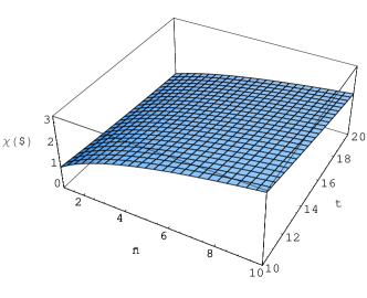
Figure 1: $\overline{n}$ ranges from $1$ to $10$ while $\gamma$ and $\beta$ are fixed as $0.1$ and $0.01$, respectively.

Assume $\overline{n}$ is fixed to $5$ and $\gamma$ fixed to $0.1$, while $\beta$ runs from $0.01$ to $0.1$, then we have the following diagram figure 2.;

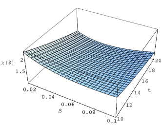
Figure 2: $\overline{n}$ is fixed to $5$ and $\gamma$ fixed to $0.1$, while $\beta$ runs from $0.01$ to $0.1$.

If $\overline{n}$ is fixed to $5$ and $\beta$ is fixed to $0.01$, while $\gamma$ ranges from $0.1$ to $0.5$, then the diagram figure 3. below is obtained.

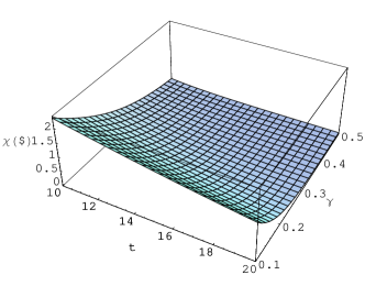
Figure 3: $\overline{n}$ is fixed to $5$ and $\beta$ is fixed to $0.01$, while $\gamma$ ranges from $0.1$ to $0.5$.

As these diagrams indicate, the channel capacity is proportional to the mean photon number at the input of the channel, yet decreases with the increase of time and intensity of noise $\beta\left(t\right)$. Here $\overline{n}$ is considered as the signal to the channel. The larger the signal, the larger the channel capacity. That the Markov quantum channel is noisy lies in the fact that $\overline{n}$ is decaying with the increase of the time. Our results are quite rational.

IV Fidelity vs. channel capacity

In quantum information theory, the fidelity is of great significance, which discusses the similarity between the input density operator and the output density operator. In some aspect, it evaluates how successful the message is transmitted and how well the channel preserves the information peters ; j ; lidar ; oh . The fidelity $\digamma$ of the channel is calculated as

$$\digamma\left(\eta\right) = \left\langle\eta\right|\rho\left(t\right)\left|\eta\right\rangle$$

$$= \left\langle\eta\right|\frac{1}{1+\beta\left(t\right)}:e^{-\frac{1}{1+\beta\left(t\right)}\left[a^{+}-\left(1+\beta\left(t\right)\right)f^{\ast}\eta^{\ast}\right]\left[a-\left(1+\beta\left(t\right)\right)f\eta\right]}:\left|\eta\right\rangle$$

$$= \frac{1}{1+\beta\left(t\right)}e^{-\left(1+\beta\left(t\right)\right)f^{2}\left|\eta\right|^{2}+f\left|\eta\right|^{2}+f^{\ast}\left|\eta\right|^{2}-\frac{1}{1+\beta\left(t\right)}\left|\eta\right|^{2}}$$

$$= \frac{1}{1+\beta\left(t\right)}\exp\left[-\frac{\left(e^{-\frac{\gamma}{2}t}-1\right)^{2}}{1+\beta\left(t\right)}\left|\eta\right|^{2}\right]$$

And the average value of $\digamma$, i.e., $\overline{\digamma}$ is

$$\overline{\digamma} = \int\frac{d^{2}\eta}{\pi\overline{n}}e^{-\frac{\left|\eta\right|^{2}}{\overline{n}}}\frac{1}{1+\beta\left(t\right)}\exp\left[-\frac{\left(e^{-\frac{\gamma}{2}t}-1\right)^{2}}{1+\beta\left(t\right)}\left|\eta\right|^{2}\right]$$

$$= \frac{1}{1+\beta\left(t\right)+\overline{n}\left(e^{-\frac{\gamma}{2}t}-1\right)^{2}}$$

It is clear that the average fidelity decreases with growing $\overline{n}$, nevertheless, the capacity increases with growing $\overline{n}$. Mathematically, we hold that there exists particular $\overline{n}_{opt}$ at which the average fidelity and the capacity are optimal, namely, certain channel capacity can be achieved with reasonably high fidelity. Below we derive the criterion for this situation.

Define $\Theta$ as

$$\Theta=\overline{\digamma}\times\chi\left(\$\right)$$

then $\overline{n}_{opt}$ must saturate the following equation

$$\frac{\partial\Theta}{\partial\overline{n}}=0$$

that is to say, $\overline{n}_{opt}$ satisfies the equation

$$a(1+\beta(t))\log(1+\beta(t))-a\beta(t)\log\beta(t)$$

$$= (a\beta(t)-(1+\beta(t)))\log b-(a-1)(1+\beta(t))\log(1+b)$$

where

$$a=\left(e^{\frac{\gamma}{2}t}-1\right)^{2}$$

$$b=\beta(t)+\overline{n}e^{-\gamma t}$$

It is evident that any signal input $\overline{n}$ saturates the criterion equation (8) above gives rise to mutually optimal channel capacity and transmission fidelity.

V Conclusions

In this paper we adopt a method to compute the quantum Markov channel of continuous variables. We use this method to calculate explicitly a noisy quantum channel with a Gaussian-distributed noise. Physically, the process is a monomodal electromagnetic field decaying inside a cavity. From the quantum information’s point of view, it is a field propagating at the prensence of reservoir.

We give the explicit form of the capacity of the channel. The channel capacity is proportional to the input signal $\overline{n}$, while decaying with the increase of time t and decaying rate $\gamma$ and the noise $\beta$.

On the other hand, the fidelity of the channel, which is a tag of the success of the information transmission, decreases with larger $\overline{n}$. Hence, there is tradeoff between fidelity and capacity. We derive the criterion when these two variables can achieve balance.

Quantum channels of continuous variables have been an important issue. We hope our research can shed light on this subject.

References

(1) M. Nielsen and I. Chuang, Quantum Computation and
Quantum Information (Cambridge University Press, Cambridge, 2000)
(2) S. L. Braunstein and A. K. Pati, Quantum Information
Theory with Continuous Variables, Kluwer, Dodrecht (2001)
(3) Thomas M. Cover and Joy A. Thomas, Elements of
Information Theory, Wiley-Interscience (August 12, 1991)
(4) C. H. Bennett and P. W. Shor, IEEE Trans.Inf. Theory
44, 2724 (1998); A. S. Holevo, arXiv:quant-ph/9809023
(5) A. S. Holevo and R. F. Werner, Phys. Rev. A 63,
032312 (2001)
(6) V. Giovannetti, S. Guha, S. Lloyd, L. Maccone, J. H.
Shapiro, and H. P. Yuen, Phys. Rev. Lett. 92, 027902 (2004);
Vittorio Giovannetti and Stefano Mancini, Phys. Rev. A 71, 062304
(2005)
(7) Chiara Macchiavello, G. Massimo Palma, and S.
Virmani, Phys. Rev. A 69, 010303(R) (2004); Nicolas J. Cerf, Julien
Clavareau, Chiara Macchiavello and Jérémie Roland, ibid.72, 042330 (2005)
(8) W. H. Zurek, Phys. Today 44(10), 36 (1991)
(9) E. Joos, H.D. Zeh, C. Kiefer, D. Giulini, K- Kupsch, I.-O.
Stamatescu, Decoherence and the Appearance of a Classical
World in Quantum Theory, Springer (July 15, 2003)
(10) Sonja Daffer, Krzysztof Wódkiewicz, and John K. McIver,
Phys. Rev. A 67, 062312 (2003); Sonja Daffer, Krzysztof Wódkiewicz, James D. Cresser, and John K. McIver, ibid, 70,
010304 (2004)
(11) A. T. Bharucha-Reid, Elements of the Theory of
Markov Processes and Their Applications (Dover Publications; April
9, 1997)
(12) John Preskill, Quantum Information and Computation (California Institute of Technology, September, 1998)
(13) A. S. Holevo, IEEE Trans. Inf. Theory 44, 269
(1998); P. Hausladen, R. Jozsa, B. Schumacher, M. Westmoreland, and W. K.
Wootters, Phys. Rev. A 54, 1869 (1996); B. Schumacher and M. D.
Westmoreland, Phys. Rev. A 56, 131 (1997)
(14) Marlan O.Scully and M.Suhail Zubairy, Quantum Optics (Cambridge 1997)
(15) D. F. Walls and G. J. Milburn, Quantum Optics
(Springer-Verlag, Berlin/Heidelberg, 1994)
(16) H.X. Lu, J. Yang, Y.D. Zhang and Z.B. Chen, Phys. Rev. A
67, 024101 (2003)
(17) N. A. Peters, T.-C. Wei, and P. G. Kwiat, Phys. Rev. A
70, 052309 (2004)
(18) J. Fiurásek, Phys. Rev. A 70, 032308 (2004)
(19) P. Zanardi and D. A. Lidar, Phys. Rev. A 70, 012315
(2004)
(20) S. Oh, S. Lee, and H.-w. Lee, Phys. Rev. A 66, 022316
(2002)