Self-Testing of Quantum Circuits

Abstract

We prove that a quantum circuit together with measurement apparatuses and EPR sources can be fully verified without any reference to some other trusted set of quantum devices. Our main assumption is that the physical system we are working with consists of several identifiable sub-systems, on which we can apply some given gates locally.

To achieve our goal we define the notions of simulation and equivalence. The concept of simulation refers to producing the correct probabilities when measuring physical systems. To enable the efficient testing of the composition of quantum operations, we introduce the notion of equivalence. Unlike simulation, which refers to measured quantities (i.e., probabilities of outcomes), equivalence relates mathematical objects like states, subspaces or gates.

Using these two concepts, we prove that if a system satisfies some simulation conditions, then it is equivalent to the one it is purposed to implement. In addition, with our formalism, we can show that these statements are robust, and the degree of robustness can be made explicit (unlike the robustness results of [DMMS00]). In particular, we also prove the robustness of the EPR Test [MY98]. Finally, we design a test for any quantum circuit whose complexity is linear in the number of gates and qubits, and polynomial in the required precision.

1 Introduction

We develop techniques for verifying the operations that a given set of quantum gates perform. We consider “self”-tests, which are tests using the given set of gates without reference to some other trusted and already characterized quantum devices. This notion was initially defined for classical programs [BK95, BLR93]. Self-testing was then extended to quantum devices [MY98, DMMS00] and to quantum testers of logical properties [BFNR03, FMSS03].

The work by Mayers and Yao [MY98] focuses on testing entangled EPR states shared between two distinguishable locations, $A$ and $B$. Apart from assuming the standard axioms of quantum mechanics, the main assumptions they exploit are locality in the sense that the measurements at $A$ commute with the measurements at $B$ (i.e., no instantaneous signaling); and that one can perform independent repetitions of the same experiments, in order to gather statistics (i.e., the apparatuses have no memory of previous runs of the experiments). However, they do not assess the robustness of their results (i.e., they do not claim that if the state satisfies the required statistics with precision $\varepsilon$ then the state is within $\varepsilon^{\Omega(1)}$ of an EPR state). Robustness is nonetheless an interesting property very much worth studying for practical reasons: first, one can never learn any statistics with infinite precision by sampling only; second, by their very nature, physical implementations are only approximate.

The work of Van Dam, Magniez, Mosca and Santha [DMMS00] focuses instead on testing gates. They make a number of assumptions, including (and in addition to assuming the standard axioms of quantum mechanics) (1) the ability to repeat the same gate in the same experiment; (2) the absence of memory in the apparatus between different experiments; (3) the ability to prepare and measure ‘0’ and ‘1’; (4) the locality of each of the gates (i.e., they only affect the qubits they are suppose to act upon); and (5) the dimension of the physical qubits (i.e., 2-level systems). Of these assumptions, the last one is certainly the most unrealistic one, but also the most crucial one. Relaxing it allows for “conspiracies” that can spoof the test, and it is not so clear how to work around them (See Appendix A for an example given by Wim van Dam).

This paper improves upon the Mayers and Yao results [MY98] by making them robust. It also improves upon the Van Dam, Magniez, Mosca and Santha paper [DMMS00] by removing the need for assumptions (1), (3) and (5). Some version of assumption (2) seems necessary. We suspect, one might be able to relax assumption (4) to some extent, but we keep a version of it in this work.

We have sketched the assumptions of the previous work that we do not wish to make. Let us now detail the assumptions that we do make. We assume that, (H1) the physical system we are working with consists of several identifiable sub-systems; (H2) two subsystems interact only if we are applying a gate that has both those subsystems as input; (H3) each gate will behave identically in each experiment it is used in (i.e., each gate is some fixed completely positive superoperator); and (H4) classical computation and control are perfect and can be trusted (e.g., classical control has no side-channel).

Our procedure allows us to test physical implementations of unitary gates, EPR creation gates, and one-qubit projective measurements. A more general superoperator can be tested by viewing it as a composition of operations of the above form.

There is however one important restriction to the class of gates we are able to test. The ideal gates must have real valued coefficients. Note that we are not making any assumptions about the physical implementation of gates, but rather on the ideal gates they are supposed to simulate. We are merely saying that we do not have a procedure for verifying that a physical gate is equivalent to a complex gate. This is not for a lack of trying. The problem is that any complex gate of dimension $d$ can be simulated using quantum systems of dimension $2d$, real gates and appropriate measurement devices, in a rather standard way [RG02]. On the positive side, this remark means that our restriction is not a limitation. But, this also means that one cannot tell if a gate is complex or simulated by a real one without external help (e.g., knowledge of the dimensionality of quantum systems, trusted one-qubit measuring apparatuses, etc.). More importantly, given any set of quantum gates, and a set of experiments attempting to characterize those gates, there is a corresponding set of real gates that would produce identical predictions. However, these two sets of gates are not equivalent according to the natural notion of equivalence we define (which is a type of local unitary equivalence). That is, we believe that such gates cannot be trusted in a cryptographic context without further assumption. The reason is that although the real-gate simulations of the complex gates yield identical outcome probabilities, an adversary might be able to take advantage of the structure of real-state simulations in order to extract information on the quantum operations being performed.

Our first contribution (Section 2) is to propose a theory of self-testing by introducing appropriate notions such as simulation and equivalence. Unlike simulation, which refers to measured quantities (i.e., probabilities of outcomes), equivalence relates mathematical objects like states, subspaces or gates. Equivalence is meant to relate objects with similar observable properties. Therefore, we have based this notion on the existence of unitary transformations that map states and operations onto their respective ideal version. Our notion preserves the inner product and hence the distinguishability of quantum states, which is a crucial tool for assessing the security of physical implementations of most quantum cryptographic protocols.

Our second contribution (Section 3) is a characterization of unitary gates and circuits. Namely, we explain how simulation implies equivalence. The main tool for thwarting conspiracies is the Mayers-Yao test of an EPR pair. We will build upon the fact that one way of preparing trusted random BB84 states is to first prepare an EPR state, transmit one half, and independently measure the other half. We will show that this method can be generalized and yields trusted input states to be used in conjunction with self-testable quantum circuits.

Our last contribution (Section 4) is to prove the robustness of our characterization. In particular, we show that the EPR test of [MY98] is robust. Using the concepts of simulation and equivalence, such proofs are not so difficult although the robustness of the EPR test had been left open. The crucial point was to realize that the robustness of our characterization needs only to be stated on a rather small subspace in order for it to be of practical interest.

The important consequence of our study is the possibility of defining a tester (Section 5) that might be used in real-life situations. Contrary to tomography which requires trusted measurement devices and an exponential number of statistics to be checked, our test has a complexity linear in the number of qubits and gates involved in the circuit, and polynomial in the required precision. We describe our tester with an example and in a general context.

2 Testing Concepts

2.1 Notation

In this section, we describe our theory of testing using a fixed integer $N$ as parameter. Later in the paper, we will set $N=2$ as it will correspond to the case of qubits. For an introduction to quantum computing, we refer the reader to [NC00, KSV02].

We denote by $\mathcal{U}(N)$ the set of unitary matrices of size $N$, $\mathcal{U}(H)$ the set of unitary transformations on the Hilbert space $H$, and $\mathcal{I}(H,H^{\prime})$ the set of isomorphisms between the Hilbert spaces $H$ and $H^{\prime}$ (with same dimension) which preserve the inner product. In case of transformations over real spaces, we use the notations $\mathcal{O}(N)$ and $\mathcal{O}(H)$ instead of $\mathcal{U}(N)$ and $\mathcal{U}(H)$.

For the Hilbert space $\mathcal{H}_{2}$ we denote by $\lvert 0\rangle$ and $\lvert 1\rangle$ the computational basis, and for any $\alpha\in\mathbb{R}$ the state $\lvert\alpha\rangle=\cos\alpha\lvert 0\rangle+\sin\alpha\lvert 1\rangle$. In particular $\lvert\tfrac{\pi}{2}\rangle=\lvert 1\rangle$. We denote by $\lvert\phi^{+}\rangle$ the EPR state $\frac{1}{\sqrt{2}}(\lvert 0\rangle\otimes\lvert 0\rangle+\lvert 1\rangle\otimes\lvert 1\rangle)$. For $n$ finite, we denote by $\lvert\Phi^{+}_{n}\rangle$ the state corresponding to $n$ EPR states: $\lvert\Phi^{+}_{n}\rangle=\frac{1}{\sqrt{2^{n}}}\sum_{x\in\{0,1\}^{n}}\lvert x\rangle\otimes\lvert x\rangle$.

For linear transformations $M$ and $M^{\prime}$ on $H$, and a subspace $S$ of $H$, the notation $M=_{S}M^{\prime}$ means that the equality holds only on $S$. When $M$ is a linear transformation on $A$, we extend $M$ on any tensor product $A\otimes B$ by $M\otimes\mathrm{Id}_{B}$; we sometimes still denote this as $M$ in an attempt to simplify our notation.

2.2 Simulation

The concept of simulation formalizes the idea of producing the correct probabilities when observing physical systems. Observations are based on fixed experimental setups comprising measuring devices that gather information about the state of the system of interest. Likewise, the simulation of a state by another one will be defined with respect to projectors. These projectors are used here in the same way measurement devices are used in a laboratory: they act as reference systems against which the system of interest is tested.

More precisely, we are given a family of projectors $(P^{w})_{w\in\mathcal{W}}$ acting on $H$, and a state $\lvert\psi\rangle$ whose purpose is to simulate the state $\lvert\phi\rangle$ of the canonical Hilbert space $\mathcal{H}_{N}=\mathbb{C}^{N}$. In the following definition, and throughout the rest of this paper, we implicitly use the labels $w$ of the projectors $P^{w}$ on $H$ to label some projectors $\lvert w\rangle\!\langle w\rvert$ on $\mathcal{H}_{N}$, that are assumed to be given and fixed.

Definition 1.

A quantum state $\lvert\psi\rangle\in H$ simulates the quantum state $\lvert\phi\rangle\in\mathcal{H}_{N}$ (with respect to $\{P^{w}\}_{w\in\mathcal{W}}$), if $\lVert P^{w}\lvert\psi\rangle\rVert^{2}=\lvert\langle w|\phi\rangle\rvert^{2}$, for every $w\in\mathcal{W}$.

The notion of simulation can be rephrased for a whole Hilbert space $H$. Let $(\lvert i\rangle)_{i}$ be the canonical orthogonal basis of $\mathcal{H}_{N}$, usually the computational basis. Assume we are given a family of states $(\lvert\psi_{i}\rangle)_{i}$ of $H$ such that each $\lvert\psi_{i}\rangle$ simulates $\lvert i\rangle$ (with respect to fixed set of projectors $\{P^{w}\}_{w\in\mathcal{W}}$). In such case, we say that $(\lvert\psi_{i}\rangle)_{i}$ simulates $(\lvert i\rangle)_{i}$ or, when there is no ambiguity, that $H$ simulates $\mathcal{H}_{N}$.

With this definition of simulation for Hilbert spaces, it is possible to extend the notion of simulation to gates. Note in the definition below that the set of projectors used to assess that $H$ simulates $\mathcal{H}_{N}$ is the same as the one used to assess that $G\lvert\psi_{i}\rangle$ simulates $T\lvert i\rangle$.

Definition 2.

Assume that $H$ simulates $\mathcal{H}_{N}$: $(\lvert\psi_{i}\rangle)_{i}$ simulates $(\lvert i\rangle)_{i}$ (with respect to $\{P^{w}\}_{w\in\mathcal{W}}$). A unitary transformation $G\in\mathcal{U}(H)$ simulates the unitary transformation $T\in\mathcal{U}(\mathcal{H}_{N})$, if $G\lvert\psi_{i}\rangle$ simulates $T\lvert i\rangle$ (with respect to $\{P^{w}\}_{w\in\mathcal{W}}$), for every $i$.

2.3 Equivalence

One goal of testing is to ensure, using few resources, that a physical implementation of a circuit is faithful enough so that the probabilities for the final measurement outcomes are identical to those that would be obtained after running the ideal circuit. Unfortunately, the notion of simulation as defined earlier does not compose. That is, measuring probabilities for parts of the circuit does not guarantee that the whole will function according to its ideal specifications. To be able to compose statements, we introduce the notion of equivalence.

Clearly, we want a notion of equivalence that respects the inner product of quantum states and that preserves the tensor product structure of the different registers. The first requirement follows from the fact that we want to be able to conclude that equivalence implies simulation and leads to an equivalence notion based on isometries or unitary transformations. The second requirement is imposed in order to keep a track of local transformations. This is crucial in this work since a series of local tests based on EPR pairs will be designed in order to test a whole circuit given by a sequence of local gates. It can be seen quite simply through the following example that using only isometries or unitary transformations does not satisfy this last property.

Consider two $4$-dimensional vector spaces $A$ and $B$, and $H=A\otimes B$. We identify in $A$ (resp. $B$) two $1$-qubit registers that we denote by $A_{1}$ and $A_{2}$ (resp. $B_{1}$ and $B_{2}$). Let $\lvert\psi\rangle=\lvert\phi^{+}\rangle_{A_{1}B_{1}}\otimes\lvert\phi^{+}\rangle_{A_{2}B_{2}}$. If the measurements on $A$ (resp. $B$) only measure the $A_{1}$-part of $A$ (resp. the $B_{1}$-part of $B$), we would like to say that $\lvert\psi\rangle$ is equivalent to $\lvert\phi^{+}\rangle$ on the subspace $S=\{\lvert\varphi\rangle_{A_{1}B_{1}}\otimes\lvert\phi^{+}\rangle_{A_{2}B_{2}}:\lvert\varphi\rangle_{A_{1}B_{1}}\in A_{1}\otimes B_{1}\}$, since the $(A_{2}\otimes B_{2})$-part of the system is not used. Even if there exists an isometry $U\in\mathcal{I}(S,\mathcal{H}_{4})$ such that $U\lvert\psi\rangle=\lvert\phi^{+}\rangle$ (and $P^{a,b}=_{S}U^{\dagger}\lvert a,b\rangle\!\langle a,b\rvert U$) this isometry cannot be decomposed with respect to the tensor decomposition of $H$. However this is fundamental for our purposes. This justifies a more elaborated notion of equivalence where we introduce a logical counterpart to any Hilbert space.

The equivalence notion we now introduce is based on the work of Mayers and Yao [MY98]. It is a mathematical notion based on the possibility of transferring states which lie within a given subspace of $H$ into a logical system $H_{c}$ prepared in a fiducial state via a joint unitary transformation.

For a Hilbert space $H$, that will describe the state of our physical system, we set a logical space $H_{c}=\mathcal{H}_{N}$ and define $\bar{H}=H_{c}\otimes H$. We consider in $H_{c}$ the usual canonical basis $(\lvert i\rangle)_{0\leq i<N}$, so that we have a canonical mapping between $H_{c}$ and $\mathcal{H}_{N}$, between $\mathcal{U}(H_{c})$ and $\mathcal{U}(N)$, and between $\mathcal{O}(H_{c})$ and $\mathcal{O}(N)$. Note that it is more convenient to set this logical system outside the physical system (instead of as a subpart of it) since initially we do not know which part of the physical system is used for the computation. Identifying some subsystem of $H$ as the logical space seems more unnatural than just adding this additional logical qubit.

The state $\lvert\psi\rangle\in H$ is embedded in $\bar{H}$ using the isometry: $\mathbb{I}_{H}:\lvert\psi\rangle\mapsto\lvert 0\rangle\otimes\lvert\psi\rangle$. The reverse operation is obtained by applying: $\mathbb{P}_{H}:\lvert\psi\rangle\mapsto\operatorname{\mathrm{tr}}_{\mathcal{H}_{N}}((\lvert 0\rangle\!\langle 0\rvert\otimes\mathrm{Id}_{H})\lvert\psi\rangle)$. It can be checked that $\mathbb{P}_{H}\mathbb{I}_{H}=\mathrm{Id}_{H}$. The operators $\mathbb{P}_{H}$ and $\mathbb{I}_{H}$ allow to identify $H$ with the subspace $\lvert 0\rangle\otimes H$ of $\bar{H}$. Similarly, any linear map $M$ on $H$ is extended to the linear map $\lvert 0\rangle\!\langle 0\rvert\otimes M$ on $\bar{H}$. Thus, we will omit $\mathbb{P}_{H}$ and $\mathbb{I}_{H}$ when there is no ambiguity.

First, we define the equivalence between a subspace of $H$ and the logical system $H_{c}$ with respect to a set of projectors. As for the notion of simulation, these projectors act as reference systems.

Definition 3.

Let $U\in\mathcal{U}(\bar{H})$. A subspace $S$ of $H$ is $U$-equivalent to $H_{c}$ (with respect to $(P^{w})_{w\in\mathcal{W}}$), if for every $w\in\mathcal{W}$, $P^{w}=_{S}\mathbb{P}_{H}U^{\dagger}(\lvert w\rangle\!\langle w\rvert\otimes\mathrm{Id}_{H})U\mathbb{I}_{H}$.

The above definition is equivalent to the commutative diagram:

$$\begin{array}[]{rcl}S&\xrightarrow{P^{w}}&S\\ U\mathbb{I}_{H}\downarrow&&\uparrow\mathbb{P}_{H}U^{\dagger}\\ \bar{H}&\xrightarrow{\lvert w\rangle\!\langle w\rvert\otimes\mathrm{Id}_{H}}&\bar{H}\end{array}.$$

Intuitively, the unitary transformation $U$ ensures that the correspondence between the physical system $H$ and the logical system $H_{c}$ is well defined on $S$. Using this correspondence, we can now define the notion of $U$-equivalence for states and gates.

Definition 4.

Let $S$ be a subspace of $H$. A state $\lvert\psi\rangle\in S$ is $U$-equivalent to a state $\lvert\phi\rangle\in H_{c}$ on $S$ (with respect to $(P^{w})_{w\in\mathcal{W}}$), if

1. $S$ is $U$-equivalent to $H_{c}$,

2. $\lvert\psi\rangle=U^{\dagger}(\lvert\phi\rangle\otimes\lvert\chi\rangle)$, for some $\lvert\chi\rangle\in H$.

Definition 5.

Let $S$ be a subspace of $H$. A unitary transformation $G\in\mathcal{U}(H)$ is $(U,V)$-equivalent to a unitary transformation $T\in\mathcal{U}(H_{c})$ on $S$ (with respect to $(P^{w})_{w\in\mathcal{W}}$), if

1. $S$ is $U$-equivalent to $H_{c}$,

2. $S^{\prime}=G(S)$ is $V$-equivalent to $H_{c}$,

3. $G=_{S}V^{\dagger}(T\otimes W)U$, for some $W\in\mathcal{U}(H)$.

This equivalence can be summarized by the following commutative diagram:

$$\begin{array}[]{rcccccl}S&\xrightarrow{P^{w}}&S&\xrightarrow{G}&S^{\prime}&\xrightarrow{P^{w}}&S^{\prime}\\ U\mathbb{I}_{H}\downarrow&&\mathbb{P}_{H}U^{\dagger}\uparrow\downarrow U\mathbb{I}_{H}&&\mathbb{P}_{H}V^{\dagger}\uparrow\downarrow V\mathbb{I}_{H}&&\uparrow\mathbb{P}_{H}V^{\dagger}\\ \bar{H}&\xrightarrow{\lvert w\rangle\!\langle w\rvert\otimes\mathrm{Id}_{H}}&\bar{H}&\xrightarrow{T\otimes W}&\bar{H}&\xrightarrow{\lvert w\rangle\!\langle w\rvert\otimes\mathrm{Id}_{H}}&\bar{H}\end{array}.$$

When $H$ is explicitly decomposed into a tensor product, $H=\bigotimes_{i=1}^{n}H^{i}$, and $P^{w}=\bigotimes_{i=1}^{n}P_{H^{i}}^{w^{i}}$, where $w=(w^{1},w^{2},\ldots,w^{n})\in\mathcal{W}^{1}\times\mathcal{W}^{2}\ldots\mathcal{W}^{n}$, we will often use the notion of equivalence for unitary matrices $U$ that can be tensor product decomposed as $U=\bigotimes_{i}U^{i}$, for some $U^{i}\in\mathcal{U}(\bar{H}^{i})$. When we do not want to specify the decomposition of $U$, we will use the notion of tensor equivalence. Notice that for the state and transformation tensor equivalence, $\lvert\chi\rangle$ and $W$ are not required to be tensor product decomposable. This is because we want encompass situations where the physical implementation $G$ of the gate creates or destroys entanglement in the hidden degrees of freedom of the quantum register.

Finally, note that the tensor equivalence on $H$ implies the equivalence for each factor $H_{i}$ of the tensor decomposition of $H$, if for each factor $H_{i}$ one can sum up some projections $P_{H^{i}}^{w^{i}}$ to the identity. This will be the case in the rest of the paper.

Proposition 1.

Let $H=\bigotimes_{i=1}^{n}H^{i}$. Let $S$ be a subspace of $H$ which is $(\bigotimes_{i}U_{i})$-equivalent to $H_{c}=\bigotimes_{i}{H^{i}_{c}}$ with respect to $(P^{w})_{w}$. Assume that for every $i$, a subset of the projectors of $(P_{H^{i}}^{w^{i}})_{w^{i}\in\mathcal{W}^{i}}$ sums to the identity on $H^{i}$. Then $S$ is $U_{i}$-equivalent to $H_{c}$ with respect to $(P_{H^{i}}^{w^{i}})_{w^{i}\in\mathcal{W}^{i}}$, for every $i$. Moreover if $S=\bigotimes_{i}S^{i}$, where $S^{i}$ is a subspace of $H^{i}$, then $S^{i}$ is $U_{i}$-equivalent to $H^{i}_{c}$ with respect to $(P_{H^{i}}^{w^{i}})_{w^{i}\in\mathcal{W}^{i}}$, for every $i$.

From now on, we set $N=2$ when we do not explicitly state otherwise. When we omit the parameters $U$ or $(U,V)$ from the equivalence notation, we mean that there exists such unitary transformations for which the $U$-equivalence or the $(U,V)$-equivalence holds.

2.4 EPR Test

In this section, we summarize Mayers and Yao’s results [MY98] in the framework of quantum testing we have just introduced. Their main result [MY03, Thm. 1] will be stated in an extended form that is most convenient for testing several registers successively.

From now and until the end of the paper, let $\mathcal{A}_{0}=\{0,\tfrac{\pi}{8},\tfrac{\pi}{4}\}$, $\mathcal{A}_{1}=\{a+\tfrac{\pi}{2}:a\in\mathcal{A}_{0}\}$, and $\mathcal{A}=\mathcal{A}_{0}\cup\mathcal{A}_{1}$. We fix in this section $(P_{A}^{a},P_{A}^{a+\pi/2})_{a\in\mathcal{A}_{0}}$ and $(P_{B}^{b},P_{B}^{b+\pi/2})_{b\in\mathcal{A}_{0}}$ orthogonal measurements respectively on two Hilbert spaces $A$ and $B$. Namely, we assume that $P_{A}^{a}+P_{A}^{a+\pi/2}=\mathrm{Id}_{A}$ and $P_{B}^{a}+P_{B}^{a+\pi/2}=\mathrm{Id}_{B}$, for every $a\in\mathcal{A}_{0}$.

Theorem 1.

Let $H=A\otimes B\otimes C$, and $\lvert\psi\rangle\in H$ that simulates $\lvert\phi^{+}\rangle$ with respect to $(P_{A}^{a}\otimes P_{B}^{b}\otimes\mathrm{Id}_{C})_{a,b\in\mathcal{A}}$. Then there exist two unitary transformations $U_{\bar{A}}\in\mathcal{U}(\bar{A})$ and $U_{\bar{B}}\in\mathcal{U}(\bar{B})$ such that $\lvert\psi\rangle$ is $(U_{\bar{A}}\otimes U_{\bar{B}})$-equivalent to $\lvert\phi^{+}\rangle$ on $S=\operatorname{\mathrm{span}}\{P_{A}^{a}\otimes P_{B}^{b}\otimes\mathrm{Id}_{C}\lvert\psi\rangle:a,b\in\mathcal{A}\}$. Moreover the dimension of $S$ is 4.

Note that the theorem can be extended from $S$ to the supports of $\lvert\psi\rangle$ on the $A$-side and on the $B$-side using [MY03, Prop. 4]. Since we will only need the result on $S$, and because the robustness the EPR test is easier to state in such case, we will only state our results for $S$, even though all of them can be extended to the tensor product of the respective supports (for the exact case).

From Theorem 1 it is easy to derive by induction over $n$ our main tool for testing $n$-qubit registers. Let $A=\bigotimes_{i=1}^{n}A^{i}$ and $B=\bigotimes_{i=1}^{n}B^{i}$, we now fix $(P_{A^{i}}^{a^{i}},P_{A^{i}}^{a^{i}+\pi/2})_{a^{i}\in\mathcal{A}_{0}}$ and $(P_{B^{i}}^{b^{i}},P_{B^{i}}^{b^{i}+\pi/2})_{b^{i}\in\mathcal{A}_{0}}$ to be orthogonal measurements on $A^{i}$ and $B^{i}$ respectively for every $i$. We denote $P_{A}^{a}=\bigotimes_{i=1}^{n}P_{A^{i}}^{a^{i}}$, with $a=(a^{i})_{i=1}^{n}$ and $P_{B}^{b}=\bigotimes_{i=1}^{n}P_{B^{i}}^{b^{i}}$ with $b=(b^{i})_{i=1}^{n}$. Note that in the following corollary, the tensor equivalence is with respect to the tensor decomposition $A\otimes B$, but also with respect to the tensor decompositions $A=\bigotimes_{i=1}^{n}A^{i}$ and $B=\bigotimes_{i=1}^{n}B^{i}$.

Corollary 1.

Let $H=A\otimes B\otimes C$, and $\lvert\Psi\rangle\in H$ that simulates $\lvert\phi^{+}\rangle$ with respect to $(P_{A^{i}}^{a^{i}}\otimes P_{B^{i}}^{b^{i}}\otimes\mathrm{Id}_{C})_{a^{i},b^{i}\in\mathcal{A}}$ for every $i=1,2,\ldots,n$. Then there exist two unitary transformations $U_{\bar{A}}\in\bigotimes_{i}\mathcal{U}(\bar{A}^{i})$ and $U_{\bar{B}}\in\bigotimes_{i}\mathcal{U}(\bar{B}^{i})$ such that $\lvert\Psi\rangle$ is $(U_{\bar{A}}\otimes U_{\bar{B}})$-equivalent to $\lvert\Phi^{+}_{n}\rangle$ on $S=\operatorname{\mathrm{span}}\{P_{A}^{a}\otimes P_{B}^{b}\lvert\psi\rangle:a,b\in\mathcal{A}^{n}\}$. Moreover the dimension of $S$ is $4^{n}$.

Therefore, when measurements are acting on different factors of the tensor product decompositions of $A$ and $B$, testing a $2n$-qubit EPR state can be done by testing the $n$ EPR pairs that are present in it. That is, by checking the probabilities of $O(n)$ outcomes, whereas there are $2^{O(n)}$ possible joint measurement outcomes.

3 Simulation implies Equivalence

In this section we relate simulation and equivalence. While it is clear that equivalence implies simulation, we show below that under certain assumptions, simulation implies equivalence. To ease the presentation of our results, we start by describing how $1$-qubit real gates, namely transformations in $\mathcal{O}(2)$, can be tested. As a second step, we show how to test $n$-qubit real gates.

3.1 One-qubit Gate Testing

As a first attempt, we show how to test that a gate is acting as the identity.

Proposition 2.

Let $H=A\otimes B$ and $G\in\mathcal{U}(A)$. Let $\lvert\psi\rangle\in H$ be such that $\lvert\psi\rangle$ and $G\lvert\psi\rangle$ simulate $\lvert\phi^{+}\rangle$. Then, $G\otimes\mathrm{Id}_{B}$ is tensor equivalent to $\mathrm{Id}_{A_{c}}\otimes\mathrm{Id}_{B_{c}}$ on $S=\operatorname{\mathrm{span}}\{P_{A}^{a}\otimes P_{B}^{b}\lvert\psi\rangle:a,b\in\mathcal{A}\}$.

Proof.

We show below that $G$ is $(U_{\bar{A}}\otimes U_{\bar{B}},U_{\bar{A}}G^{\dagger}\otimes U_{\bar{B}})$-equivalent to $\mathrm{Id}_{A_{c}}\otimes\mathrm{Id}_{B_{c}}$ on $S$.

First note that Lemmas 1 and 2 applied to $\lvert\psi\rangle$ gives $U_{\bar{A}}$ and $U_{\bar{B}}$ such that $S$ is $(U_{\bar{A}}\otimes U_{\bar{B}})$-equivalent to $A_{c}\otimes B_{c}$ and $U_{\bar{A}}\otimes U_{\bar{B}}\lvert\psi\rangle=\lvert\phi^{+}\rangle\otimes\lvert\chi\rangle$ for some $\lvert\chi\rangle$ in $A\otimes B$. We can derive that $(U_{\bar{A}}G^{\dagger}\otimes U_{\bar{B}})G\lvert\psi\rangle=\lvert\phi^{+}\rangle\otimes\lvert\chi\rangle$.

Hence, it only remains to show that $G(S)$ is $(U_{\bar{A}}G^{\dagger}\otimes U_{\bar{B}})$-equivalent to $A_{c}\otimes B_{c}$. Let $a,b,a^{\prime},b^{\prime}\in\mathcal{A}$, then the following equalities hold:

$$(P_{A}^{a}\otimes P_{B}^{b})(G\otimes\mathrm{Id}_{B})(P_{A}^{a^{\prime}}\otimes P_{B}^{b^{\prime}})\lvert\psi\rangle =(\mathrm{Id}_{A}\otimes P_{B}^{b}P_{B}^{b^{\prime}}P_{B}^{a^{\prime}})(P_{A}^{a^{\prime}}G\otimes\mathrm{Id}_{B})\lvert\psi\rangle$$

$$=G\otimes P_{B}^{b}P_{B}^{b^{\prime}}P_{B}^{a^{\prime}}P_{B}^{a}\lvert\psi\rangle$$

$$=(G\otimes\mathrm{Id}_{B})(P_{A}^{a}\otimes P_{B}^{b})(P_{A}^{a^{\prime}}\otimes P_{B}^{b^{\prime}})\lvert\psi\rangle,$$

where we applied Proposition 3 (see Appendix B.2) to $\lvert\psi\rangle$ on the first and the last line, and to $G\lvert\psi\rangle$ on the second line. In other words, this states that $(P_{A}^{a}\otimes P_{B}^{b})(G\otimes\mathrm{Id}_{B})=_{S}(G\otimes\mathrm{Id}_{B})(P_{A}^{a}\otimes P_{B}^{b})$. Using $U_{A}\otimes U_{B}$ to replace $P_{A}^{a}\otimes P_{B}^{b}$ over $S$, we get $P_{A}^{a}\otimes P_{B}^{b}=_{G(S)}(GU_{\bar{A}}^{\dagger}\otimes U_{\bar{B}}^{\dagger})(\lvert a\rangle\!\langle a\rvert\otimes\lvert b\rangle\!\langle b\rvert)(U_{\bar{A}}G^{\dagger}\otimes U_{\bar{B}})$, which is the required equivalence between $G(S)$ and $A_{c}\otimes B_{c}$. ∎

Stating the above result allows us to exhibit simple characteristics of the general method used for proving that gates can be self-tested. First, any gate testing requires two EPR tests. These are used to ensure that the input and output states together with the measurements act properly before and after the gate. These are “conspiracy” tests. Second, the fundamental properties of EPR states—namely that a given measurement can be performed on either the $A$-side or the $B$-side without changing the collapsed state—is used in order to show that on the input state $\lvert\psi\rangle$, the gate $G$ and the measurements commute. Together with the replacement of the projectors $P_{A}^{a}$ and $P_{B}^{b}$, that come from the physical measurements, by their ideal versions $\lvert a\rangle\!\langle a\rvert$ and $\lvert b\rangle\!\langle b\rvert$ on $A_{c}$ and $B_{c}$, this allows to perform the tomography of the gate $G$.

We can now state the general result concerning any $1$-qubit real gate.

Theorem 2.

Let $T\in\mathcal{O}(2)$. Let $H=A\otimes B$, $G_{A}\in\mathcal{U}(A)$, and $G_{B}\in\mathcal{U}(B)$. Let $\lvert\psi\rangle\in H$ be such that $\lvert\psi\rangle$ and $G_{A}G_{B}\lvert\psi\rangle$ simulate $\lvert\phi^{+}\rangle$, and such that $G_{A}\lvert\psi\rangle$ simulates $(T\otimes\mathrm{Id}_{2})\lvert\phi^{+}\rangle$. Then, $G_{A}$ is tensor equivalent to $T$ on $S=\operatorname{\mathrm{span}}\{P_{A}^{a}\otimes P_{B}^{b}\lvert\psi\rangle:a,b\in\mathcal{A}\}$.

Proof.

The proof proceeds in two steps. First, it is shown that $S$ and $G_{A}(S)$ are respectively $(U_{\bar{A}}\otimes U_{\bar{B}})$- and $(V_{\bar{A}}\otimes U_{\bar{B}})$-equivalent to $A_{c}\otimes B_{c}$. Second, it is shown that there exists $W\in\mathcal{U}(A)$ such that $G_{A}\otimes\mathrm{Id}_{B}=_{S}(V_{\bar{A}}^{\dagger}\otimes U_{\bar{B}}^{\dagger})(T\otimes W\otimes\mathrm{Id}_{\bar{B}})(U_{\bar{A}}\otimes U_{\bar{B}})$.

Lemmas 1 and 2 applied to $\lvert\psi\rangle$ and $G_{A}G_{B}\lvert\psi\rangle$ give $U_{\bar{A}},V_{\bar{A}}\in\mathcal{U}(\bar{A})$ and $U_{\bar{B}},V_{\bar{B}}\in\mathcal{U}(\bar{B})$ such that $S$ and $(G_{A}\otimes G_{B})(S)$ are respectively $(U_{\bar{A}}\otimes U_{\bar{B}})$- and $(V_{\bar{A}}\otimes V_{\bar{B}})$-equivalent to $A_{c}\otimes B_{c}$. This implies that $(G_{A}\otimes\mathrm{Id}_{B})(S)$ is $(V_{\bar{A}}\otimes U_{\bar{B}})$-equivalent to $A_{c}\otimes B_{c}$. That is, we have the required tensor equivalences for $S$ and $G_{A}(S)$. If we define $\lvert\chi\rangle_{AB}$ as $U_{\bar{A}}\otimes U_{\bar{B}}\lvert\psi\rangle=\lvert\phi^{+}\rangle_{A_{c}B_{c}}\otimes\lvert\chi\rangle_{AB}$, we then have $S=U_{A}^{\dagger}\otimes U_{B}^{\dagger}(A_{c}\otimes B_{c}\otimes{\lvert\chi\rangle_{AB}})$.

The simulation of $T\lvert\phi^{+}\rangle$ by $G_{A}\lvert\psi\rangle$ can be rewritten within the density matrix formalism as: $\operatorname{\mathrm{tr}}\left((P_{A}^{a}\otimes P_{B}^{b})G_{A}\lvert\psi\rangle\!\langle\psi\rvert G_{A}^{\dagger}\right)=\operatorname{\mathrm{tr}}\left((\lvert a\rangle\!\langle a\rvert\otimes\lvert b\rangle\!\langle b\rvert)(T\otimes\mathrm{Id}_{2})\lvert\phi^{+}\rangle\!\langle\phi^{+}\rvert(T^{\dagger}\otimes\mathrm{Id}_{2})\right)$. Using the commutativity of the trace operator and $(\mathrm{Id}_{2}\otimes\lvert b\rangle\!\langle b\rvert)\lvert\phi^{+}\rangle\!\langle\phi^{+}\rvert=\tfrac{1}{2}\lvert b\rangle\!\langle b\rvert\otimes\lvert b\rangle\!\langle b\rvert$, we get $\operatorname{\mathrm{tr}}\left((G_{A}^{\dagger}P_{A}^{a}G_{A}\otimes P_{B}^{b})\lvert\psi\rangle\!\langle\psi\rvert\right)=\frac{1}{2}\operatorname{\mathrm{tr}}\left(T^{\dagger}\lvert a\rangle\!\langle a\rvert T\lvert b\rangle\!\langle b\rvert\right)$.

Define the positive semi-definite operator $R^{a}_{\bar{A}\bar{B}}=(U_{\bar{A}}\otimes U_{\bar{B}})G_{A}^{\dagger}P_{A}^{a}G_{A}(U_{\bar{A}}^{\dagger}\otimes U_{\bar{B}}^{\dagger})$. Since $\lvert\psi\rangle$ is tensor equivalent to $\lvert\phi^{+}\rangle$, we have: $\operatorname{\mathrm{tr}}\left(R^{a}_{\bar{A}\bar{B}}(\lvert b\rangle\!\langle b\rvert_{A_{c}}\otimes\lvert b\rangle\!\langle b\rvert_{B_{c}}\otimes\lvert\chi\rangle\!\langle\chi\rvert_{AB})\right)=\operatorname{\mathrm{tr}}\left(T^{\dagger}\lvert a\rangle\!\langle a\rvert T\lvert b\rangle\!\langle b\rvert\right)$.

This can easily yield the equations required to apply Lemma 5 for performing the tomography of $R^{a}_{\bar{A}\bar{B}}$. For instance, observe that the operators $U_{\bar{B}}$ and $U_{\bar{B}}^{\dagger}$ can be removed from the definition of $R^{a}_{\bar{A}\bar{B}}$ without modifying it. Therefore the previous equation can be extended for all $b,b^{\prime}\in\mathcal{A}$ to

$$\operatorname{\mathrm{tr}}\left(R^{a}_{\bar{A}\bar{B}}(\lvert b\rangle\!\langle b\rvert_{A_{c}}\otimes\lvert b^{\prime}\rangle\!\langle b^{\prime}\rvert_{B_{c}}\otimes\lvert\chi\rangle\!\langle\chi\rvert_{AB})\right)=\operatorname{\mathrm{tr}}\left(T^{\dagger}\lvert a\rangle\!\langle a\rvert T\right),$$

since the value of the left hand side does not depend on $b^{\prime}$.

Now Lemma 5 can be applied on $A_{c}$ to the operators ${}_{AB}\langle\chi\rvert{}_{B_{c}}\langle b^{\prime}\rvert R^{a}_{\bar{A}\bar{B}}\lvert b^{\prime}\rangle_{B_{c}}\lvert\chi\rangle_{AB}$ and $T^{\dagger}\lvert a\rangle\!\langle a\rvert T$ with $n=1$ and $\varepsilon=0$. The conclusion is that ${}_{AB}\langle\chi\rvert{}_{B_{c}}\langle b^{\prime}\rvert R^{a}_{\bar{A}\bar{B}}\lvert b^{\prime}\rangle_{B_{c}}\lvert\chi\rangle_{AB}=(T^{\dagger}\lvert a\rangle\!\langle a\rvert T)$, for every $b^{\prime}\in\mathcal{A}$. Since $R^{a}_{\bar{A}\bar{B}}$ is a semi-definite operator, the above conclusion can be rewritten as

$$R^{a}_{\bar{A}\bar{B}}=_{A_{c}\otimes B_{c}\otimes{\lvert\chi\rangle_{AB}}}(T^{\dagger}\lvert a\rangle\!\langle a\rvert T)\otimes\mathrm{Id}_{A\otimes{\bar{B}}}.$$ (1)

The tensor-equivalence of $G_{A}(S)$ with $A_{c}\otimes B_{c}$ also gives

$$P_{A}^{a}=_{G_{A}(S)}(V_{\bar{A}}^{\dagger}\otimes U_{\bar{B}}^{\dagger})(\lvert a\rangle\!\langle a\rvert\otimes\mathrm{Id}_{A\otimes{\bar{B}}})(V_{\bar{A}}\otimes U_{\bar{B}}).$$

Since $S=U_{A}^{\dagger}\otimes U_{B}^{\dagger}(A_{c}\otimes B_{c}\otimes{\lvert\chi\rangle})$, this can be used to replace $P_{A}^{a}$ inside Equation (1). We obtain

$$(\lvert a\rangle\!\langle a\rvert\otimes\mathrm{Id}_{A\otimes{\bar{B}}})(V_{\bar{A}}\otimes U_{\bar{B}})G_{A}(U_{\bar{A}}^{\dagger}\otimes U_{\bar{B}}^{\dagger})(T^{\dagger}\otimes\mathrm{Id}_{A\otimes{\bar{B}}})\\ =_{A_{c}\otimes B_{c}\otimes{\lvert\chi\rangle}}(V_{\bar{A}}\otimes U_{\bar{B}})G_{A}(U_{\bar{A}}^{\dagger}\otimes U_{\bar{B}}^{\dagger})(T^{\dagger}\otimes\mathrm{Id}_{A\otimes{\bar{B}}})(\lvert a\rangle\!\langle a\rvert\otimes\mathrm{Id}_{A\otimes{\bar{B}}}).$$

Then, we conclude using Lemma 6 with $\varepsilon=0$, that there exists $W\in\mathcal{U}(A)$ such that

$$G_{A}=_{S}(V_{\bar{A}}^{\dagger}\otimes U_{\bar{B}}^{\dagger})(T\otimes W\otimes\mathrm{Id}_{\bar{B}})(U_{\bar{A}}\otimes U_{\bar{B}}).$$

∎

3.2 Many-qubit Gate Testing

We now consider $n$-qubit real gates. We present our main result for testing gates using a slightly different formulation than in Theorem 2. The reason for this change is that it makes the proof of the composition theorem (Theorem 4) used for self-testing circuits straightforward. We have also added an extra Hilbert space $C$ in the tensor product decomposition of $H$. The proof is omitted since it is identical to the second step of the proof of Theorem 2, where $a$, $b$ and $b^{\prime}$ are now in $\mathcal{A}^{n}$.

Theorem 3.

Let $T\in\mathcal{O}(2^{n})$. Let $H=A\otimes B\otimes C$, where $A=\bigotimes_{i}A^{i}$ and $B=\bigotimes_{i}B^{i}$. Let $G_{A}\in\mathcal{U}(A)$ and $G_{B}\in\mathcal{U}(B)$. Let $\lvert\Psi\rangle\in H$ and $U_{\bar{A}},V_{\bar{A}}\in\bigotimes_{i}\mathcal{U}(\bar{A}_{i})$ and $U_{\bar{B}},V_{\bar{B}}\in\bigotimes_{i}\mathcal{U}(\bar{B}_{i})$ be such that:

1. $\lvert\Psi\rangle$ is $(U_{\bar{A}}\otimes U_{\bar{B}})$-equivalent to $\lvert\Phi^{+}_{n}\rangle$ on $S$ with respect to $(P_{A}^{a}\otimes P_{B}^{b})_{a,b\in\mathcal{A}^{n}}$,

2. $G_{A}G_{B}\lvert\Psi\rangle$ is $(V_{\bar{A}}\otimes V_{\bar{B}})$-equivalent to $\lvert\Phi^{+}_{n}\rangle$ on $(G_{A}\otimes G_{B})(S)$ with respect to $(P_{A}^{a}\otimes P_{B}^{b})_{a,b\in\mathcal{A}^{n}}$,

3. $G_{A}\lvert\Psi\rangle$ simulates $(T\otimes\mathrm{Id}_{2^{n}})\lvert\Phi^{+}_{n}\rangle$ with respect to $(P_{A}^{a}\otimes P_{B}^{b}\otimes\mathrm{Id}_{C})_{a,b\in\mathcal{A}^{n}}$,

where $S=\operatorname{\mathrm{span}}\{P_{A}^{a}\otimes P_{B}^{b}\lvert\psi\rangle:a,b\in\mathcal{A}^{n}\}$. Then $G_{A}$ is $(U_{\bar{A}}\otimes U_{\bar{B}},V_{\bar{A}}\otimes U_{\bar{B}})$-equivalent to $T$ on $S$.

Using Corollary 1, one can observe that this formulation is not weaker than the one of Theorem 2.

3.3 Circuit Testing

Now we state our main theorem and its corollary which relates the simulation of states to the equivalence of gates, and therefore to the simulation of gates. We omit their proof due to the lack of space and because they are derived easily from Corollary 1 and Theorem 3.

Assume that some Hilbert space $H$ has a tensor product decomposition $H=\bigotimes_{i=1}^{n}A^{i}\bigotimes B^{i}$. For any subset $I\subseteq\{1,2,\ldots,n\}$, let $H^{I}$ denote the Hilbert space $\bigotimes_{i\in I}A^{i}\bigotimes_{i\in I}B^{i}$, and $\lvert\Phi^{+}\rangle_{I}$ the corresponding EPR state $\lvert\Phi^{+}_{|I|}\rangle$ over $\bigotimes_{i\in I}A_{c}^{i}\bigotimes_{i\in I}B_{c}^{i}$.

Theorem 4.

Let $H=A\otimes B$, where $A=\bigotimes_{i}A^{i}$ and $B=\bigotimes_{i}B^{i}$. Let $I^{1},I^{2},\ldots,I^{t}\subseteq\{1,2,\ldots,n\}$ be $t$ subsets. Let $G_{A}^{j}\in\mathcal{U}(A^{I^{j}})$, $G_{B}^{j}\in\mathcal{U}(B^{I^{j}})$ and $T^{j}\in\mathcal{O}(A_{c}^{I^{j}})$. Let $\lvert\Psi\rangle\in A\otimes B$. Define inductively $\lvert\Psi^{\prime j}\rangle=(G_{A}^{j}\otimes\mathrm{Id}_{B})\lvert\Psi^{j-1}\rangle$ and $\lvert\Psi^{j}\rangle=(G_{A}^{j}\otimes G_{B}^{j})\lvert\Psi^{j-1}\rangle$, where $\lvert\Psi^{0}\rangle=\lvert\Psi^{\prime 0}\rangle=\lvert\Psi\rangle$. Assume the following.

1. $\lvert\Psi\rangle$ simulates $\lvert\phi^{+}\rangle$ with respect to $(P_{A^{i}}^{a^{i}}\otimes P_{B^{i}}^{b^{i}})_{a^{i},b^{i}\in\mathcal{A}}$, for every $i=1,2,\ldots,n$.

2. For every $j=1,\ldots,t$: $\lvert\Psi^{j}\rangle$ simulates $\lvert\phi^{+}\rangle$ with respect to $(P_{A^{i}}^{a^{i}}\otimes P_{B^{i}}^{b^{i}})_{a^{i},b^{i}\in\mathcal{A}}$, for every $i\in I^{j}$.

3. For every $j=1,\ldots,t$: $\lvert\Psi^{\prime j}\rangle$ simulates $T^{j}\lvert\Phi^{+}\rangle_{I^{j}}$ with respect to $(P_{A^{I^{j}}}^{a}\otimes P_{B^{I^{j}}}^{b})_{a,b\in\mathcal{A}^{I^{j}}}$.

Then $G_{A}^{t}G_{A}^{t-1}\cdots G_{A}^{1}$ is tensor equivalent to $T^{t}T^{t-1}\cdots T^{1}$ on $S=\operatorname{\mathrm{span}}(P_{A}^{a}\otimes P_{B}^{b}\lvert\Psi\rangle:a,b\in\mathcal{A}^{n})$.

Corollary 2.

Let $\lvert\Psi\rangle\in H$ that satisfies the hypothesis of Theorem 4 for some decomposition of $G_{A}\in\mathcal{U}(A)$ and $T\in\mathcal{U}(A_{c})$ into $t$ gates acting only on a constant number of qubits. Then, for every $x\in\{0,1\}^{n}$, the state ${\sqrt{2^{n}}}\operatorname{\mathrm{tr}}_{B}(P_{B}^{x}\lvert\Psi\rangle)$ simulates $\lvert x\rangle_{A_{c}}$ with respect to $(P_{A}^{w})_{w\in\mathcal{A}^{n}}$. Moreover $G_{A}$ simulates $T$ with respect to the above identification, and the number of statistics to be checked is in $O(t)$.

4 Robustness of Simulation

4.1 Norm and Notation

We consider the $\ell_{2}$ norm $\lVert\cdot\rVert$ for states, and the corresponding operator $\lVert\cdot\rVert$ norm for linear transformations. These norms are stable by tensor product composition in the following sense: $\lVert u\otimes v\rVert=\lVert u\rVert\times\lVert v\rVert$, if $u$ and $v$ denote either vectors or linear transformations.

We note $\lvert\psi\rangle=^{\varepsilon}\lvert\psi^{\prime}\rangle$ when two vectors $\lvert\psi\rangle,\lvert\psi^{\prime}\rangle$ are such that $\lVert\lvert\psi\rangle-\lvert\psi^{\prime}\rangle\rVert\leq\varepsilon$. We extend the $\ell_{2}$-operator norm for restrictions of linear transformations on $H$. Namely if $M$ is a linear transformation on $H$, and $S$ is a subspace of $H$ we define by $\lVert M\rVert_{S}=\sup(\lVert M\lvert\psi\rangle\rVert:\lvert\psi\rangle\in S\text{ and }\lVert\lvert\psi\rangle\rVert=1)$. Similarly to states, we will write $M=^{\varepsilon}_{S}N$ when $\lVert M-N\rVert_{S}\leq\varepsilon$.

We introduce the notion of $\varepsilon$-simulation by extending the notion of simulation where statistics equalities are only approximately valid up to some additive term $\leq\varepsilon$. The notions of equivalence can be similarly extended to $\varepsilon$-equivalence, by replacing each equality $=_{S}$ by $=^{\varepsilon}_{S}$.

We will not detail the multiplicative constants that will occur in the upper bound on our additive error terms, but we will use instead the notation $O(f(\varepsilon))$ that denotes the existence of a universal constant $c$ for which the upper bound $c\times f(\varepsilon)$ is valid. We will use the notation $\Omega(f(\varepsilon))$ in a similar way.

4.2 Robustness

Until now, our interest has been focused on the possibility of self-testing a quantum circuit when outcome probabilities are known with perfect accuracy. To be of practical interest, our results must be extended to the situation of finite accuracy. We show below that it is possible and that all the relevant results for testing are indeed robust in the following way: if the statistics are close to the ideal ones, then the states, the measurements and the gates are also close to ones that are equivalent to the ideal ones. This notion of robustness follows the ones of Rubinfeld and Sudan [RS96, Rub99] for classical computing and of [DMMS00] for quantum computing.

One can extend quite easily Theorem 1 on the vector space $S=\operatorname{\mathrm{span}}(P_{A}^{a}P_{B}^{b}\lvert\psi\rangle:a,b\in\mathcal{A})$, which is enough for our purposes. Note that a robust version of Theorem 1 that would be valid on the tensor product of the supports of $\lvert\psi\rangle$ on the $A$-side and on the the $B$-side is much more difficult to state as well as inefficient in its robustness parameter $\varepsilon$. This is because its conclusion might depend on the dimensions of $A$ and $B$.

Theorem 5.

Let $H=A\otimes B\otimes C$, and $\lvert\psi\rangle\in H$ that $\varepsilon$-simulates $\lvert\phi^{+}\rangle$ with respect to $(P_{A}^{a}\otimes P_{B}^{b}\otimes\mathrm{Id}_{C})_{a,b\in\mathcal{A}}$. Then there exist two unitary transformations $U_{\bar{A}}\in\mathcal{U}(\bar{A})$ and $U_{\bar{B}}\in\mathcal{U}(\bar{B})$ such that $\lvert\psi\rangle$ is $(O({\varepsilon}^{1/4}),(U_{\bar{A}}\otimes U_{\bar{B}}))$-equivalent to $\lvert\phi^{+}\rangle$ on $S$.

The proof can be found in Appendix B. This result can be generalized to the case of a source producing a state $\lvert\Psi\rangle$ that simulates $n$ EPR pairs. In such case equivalence holds within $O(4^{n}\varepsilon)$.

Corollary 3.

Let $H=A\otimes B\otimes C$, where $A=\bigotimes_{i}A^{i}$ and $B=\bigotimes_{i}B^{i}$. Let $\lvert\Psi\rangle\in H$ be a state that $\varepsilon$-simulates $\lvert\phi^{+}\rangle$ with respect to $(P_{A^{i}}^{a^{i}}\otimes P_{B^{i}}^{b^{i}})_{a^{i},b^{i}\in\mathcal{A}}$, for every $i=1,2,\ldots,n$. Then, $\lvert\Psi\rangle$ is $O(4^{n}\varepsilon^{1/4})$-equivalent to $\lvert\Phi^{+}_{n}\rangle$.

Another corollary that we will use in the context of circuit testing concerns the case of $n$ sources of EPR pairs that are tested simultaneously. This is qualitatively different from the previous situation as the state $\lvert\Psi\rangle$ that is tested is assumed to be separable across the tensor product decomposition of $H$ into $H^{i}=A^{i}\otimes B^{i}$.

Corollary 4.

Let $H=A\otimes B\otimes C$, where $A=\bigotimes_{i}A^{i}$ and $B=\bigotimes_{i}B^{i}$. Let $\lvert\Psi\rangle\in H$ be a separable state across the tensor product decomposition of $H$ into $A_{i}\otimes B_{i}$, and such that it $\varepsilon$-simulates $\lvert\phi^{+}\rangle$ with respect to $(P_{A^{i}}^{a^{i}}\otimes P_{B^{i}}^{b^{i}})_{a^{i},b^{i}\in\mathcal{A}}$, for every $i=1,2,\ldots,n$. Then, $\lvert\Psi\rangle$ is $O(n\varepsilon^{1/4})$-equivalent to $\lvert\Phi^{+}_{n}\rangle$.

The proof of these two corollaries can be found in Appendix B. Now we concentrate on the robustness of Theorem 3 which is proven in Appendix C. Note that the exponential dependency in the number $n$ of qubits it not a constraint, since we will use this theorem for constant $n$ only (i.e., we assume an upper bound on the number of qubits affected by a gate, say $n\leq 3$).

Theorem 6.

Let $T\in\mathcal{O}(2^{n})$. Let $H=A\otimes B\otimes C$, where $A=\bigotimes_{i}A^{i}$ and $B=\bigotimes_{i}B^{i}$. Let $G_{A}\in\mathcal{U}(A)$ and $G_{B}\in\mathcal{U}(B)$. Let $\lvert\Psi\rangle\in H$ and $U_{\bar{A}},V_{\bar{A}}\in\bigotimes_{i}\mathcal{U}(\bar{A}_{i})$ and $U_{\bar{B}},V_{\bar{B}}\in\bigotimes_{i}\mathcal{U}(\bar{B}_{i})$ be such that:

1. $\lvert\Psi\rangle$ is $(\varepsilon,(U_{\bar{A}}\otimes U_{\bar{B}}))$-equivalent to $\lvert\Phi^{+}_{n}\rangle$ on $S$ with respect to $(P_{A}^{a}\otimes P_{B}^{b})_{a,b\in\mathcal{A}^{n}}$,

2. $G_{A}\otimes G_{B}\lvert\Psi\rangle$ is $(\varepsilon,(V_{\bar{A}}\otimes V_{\bar{B}}))$-equivalent to $\lvert\Phi^{+}_{n}\rangle$ on $(G_{A}\otimes G_{B})(S)$ with respect to $(P_{A}^{a}\otimes P_{B}^{b})_{a,b\in\mathcal{A}^{n}}$,

3. $G_{A}\lvert\Psi\rangle$ $\varepsilon$-simulates $(T\otimes\mathrm{Id}_{2^{n}})\lvert\Phi^{+}_{n}\rangle$ with respect to $(P_{A}^{a}\otimes P_{B}^{b}\otimes\mathrm{Id}_{C})_{a,b\in\mathcal{A}^{n}}$.

Then $G_{A}\otimes\mathrm{Id}_{B}$ is $(2^{O(n)}\sqrt{\varepsilon},(U_{\bar{A}}\otimes U_{\bar{B}},V_{\bar{A}}\otimes U_{\bar{B}}))$-equivalent to $T\otimes\mathrm{Id}_{\bar{B}_{c}}$ on $S$.

5 Testing a Circuit on a Specific Input

5.1 Construction

The assumptions we have made so far for gate testing are allowing very broad and generic conspiracies. For instance, the behavior of a gate can depend on previously applied gates in the circuit. Hence, it is impossible to have a fixed finite set of tests for characterizing the individual gates and then trust that the composition of these gates in a circuit will correctly simulate the ideal circuit. In other words, any circuit used for computation must be part of some tests.

Surprisingly, it is much easier to test the simulation of a circuit on the subspace $S$ than on a particular input. In fact, using EPR pairs allows for the simultaneous testing of all possible inputs, while making the selection of a particular one difficult. The obvious choice would be to post-select the outcome of the $B$-side measurements of the EPR pairs. Unfortunately, the selected input state would then be prepared with exponentially small probability. However, it is difficult to imagine being rid of EPR pairs as they appear to be the only kind of states that can be trusted and yet allow efficient gate testing.

We circumvent the aforementioned difficulty using the fact that our circuits can have classically controlled feedback that decides which gates need to be applied based on some measurement results. More precisely, given a circuit for a unitary transformation $T$ and an input $x$, we first measure the $B$-side of the (alleged) EPR states. This yields a classical state $y$ on the $A$-side. Second, we design a circuit $T_{x,y}$ whose purpose is to flip the corresponding bits of $y$ in order to get the input $x$, and to apply the initial circuit for $T$. Third, we run the modified circuit on the state $y$ that was prepared on the $A$-side. Finally, we test that this modified circuit implemented the correct computation. This includes verifying the gates and the preparation of all input states $\lvert x^{\prime}\rangle$—and in particular the preparation of $\lvert x\rangle$—obtained by measuring $\lvert\Psi\rangle$ on the $B$-side.

5.2 An Example

As a simple example, in Figure 1 we consider a small 2-qubit circuit that requires all-zeros as input.

We first run the computation (Experiment 1) once. Suppose the intermediate measurements on the B-side yield the outcomes $M_{1},M_{2}\in\{0,1\}$, as indicated in the diagram. The measurement outcomes determine whether $N^{0}=I$ or $N^{1}=N$ were applied to the other halves of the (alleged) EPR pairs, in order to prepare ‘0’ inputs for the initial circuit we intended to run.

We now wish to check that the output of the circuit is correct. We carry on implementing Experiments 2 through 8 each a number of times in $\log(n/\gamma)/\varepsilon^{8}$, where $\varepsilon$ is the required precision and $\gamma$ is some confidence parameter. In general, the number of different circuits to be run is linear in $t+n$, where $t$ is the number of gates in the circuit and $n$ is the number of qubits of the circuit, so we consider the test to be efficient.

The test circuits correspond to two independent sub-circuits being run on separate halves of $n$ EPR pairs. While the gate $G_{A}^{i}$ is purposed to implement the $i$-th step of the circuit, the gate $G_{B}^{i}$ should undo $G_{A}^{i}$ (by implementing the transpose gate). There are two types of tests. The “conspiracy tests” (Experiments 2,4,6,8) verify the effective dimension of the Hilbert spaces to be $2$ for each computational qubit system at each step of the circuit, and the “tomography tests” (Experiments 3,5,7) are characterizing the unitaries to confirm that they are the correct ones. Since the systems on each half of the test circuit never interact again, the gates on each side cannot “know” if they are in a conspiracy test, a tomography test, or the actual computation.

Thus, if all the conspiracy and tomography tests are passed, we are confident that the actual computation was carried out faithfully, and any ancillary states are not entangled with the output of the ideal circuit.

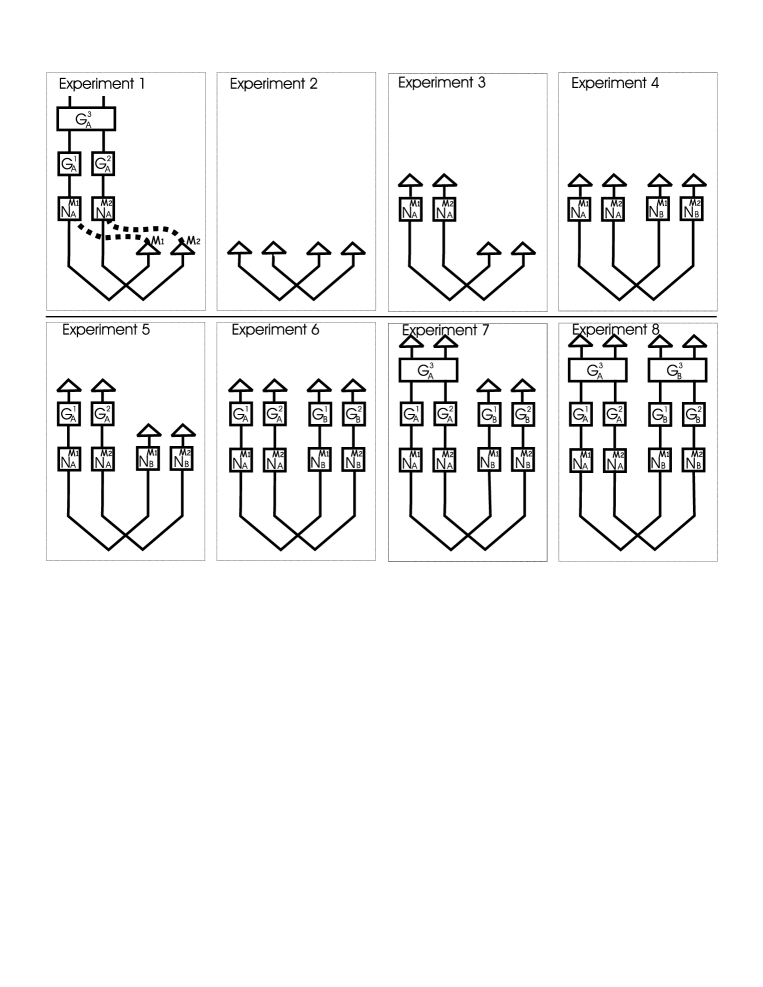
Figure 1: The different experiments to test the circuit consisting of gates $G^{3}_{A}G^{2}_{A}G^{1}_{A}$ on input $\lvert 00\rangle$.

5.3 The generic Test and its Analysis

The parameters of our test is a circuit for $T\in\mathcal{U}(2^{n})$, that is a gate decomposition $T^{t}T^{t-1}\cdots T^{1}=T$; a binary string $x\in\{0,1\}^{n}$; a precision $\varepsilon>0$; and a confidence $\gamma>0$. We assume that each gate $T^{i}$ acts on a constant number of qubits (say $\leq 3)$. The input is a source of quantum states $\lvert\Psi\rangle$ spread over $n$ pairs of quantum registers; gates $G_{A}^{j}$ and $G_{B}^{j}$ acting on the same register numbers as $T^{j}$, for every $j$; auxiliary gates $N_{A}^{i}$ acting on the $i$-th register of $A$; and orthogonal measurements $(P_{A^{i}}^{a},P_{A^{i}}^{a+\pi/2})_{a\in\mathcal{A}_{0}}$ and $(P_{B^{i}}^{b},P_{B^{i}}^{b+\pi/2})_{b\in\mathcal{A}_{0}}$. The goal is to test that, firstly, $\sqrt{2^{n}}\operatorname{\mathrm{tr}}_{B}(P^{b}_{B}\lvert\Psi\rangle)$ simulates $\lvert b\rangle$ and that, secondly, the implemented circuit $G_{A}$ simulates $T$.

Circuit Test $(T^{1},T^{2},\ldots,T^{t}\in\mathcal{U}(2^{n}),x\in\{0,1\}^{n},\varepsilon>0,\gamma>0)$ 1. Prepare a state $\lvert\Psi\rangle$ of $n$ EPR states into $n$ pairs of registers $A^{1}\otimes B^{1},\ldots,A^{n}\otimes B^{n}$ 2. Observe the $B$-side of $\lvert\Psi\rangle$ using the orthogonal measurement $(P_{B}^{b})_{b\in\{0,\pi/2\}^{n}}$ and let $y$ be the outcome 3. Let $T_{x,y}$ be the circuit that changes the input $\lvert y\rangle$ into $\lvert x\rangle$ (using some NOT gates), and then applies $T$ 4. Prepare on the $A$-side the circuit $G_{A}$ implementing $T_{x,y}$ with respect to its gate decomposition using the $t$ gates of $G_{A}^{j}$ and at most $n$ gates of $N_{A}^{i}$. Let $t^{\prime}\leq t+n$ be the total number of gates. 5. Run the circuit on the $A$-side and measure the outcome using the orthogonal measurement $(P_{A}^{a})_{a\in\{0,\pi/2\}^{n}}$ 6. Approximate all the following statistics by repeating $O(\tfrac{\log(n/\gamma)}{\varepsilon})$ times the following measurements (where we use the notation of Theorem 4): (a) Measure $\lvert\Psi\rangle$ with respect to $(P_{A^{i}}^{a^{i}}\otimes P_{B^{i}}^{b^{i}})_{a^{i},b^{i}\in\mathcal{A}_{0}}$, for every $i=1,2,\ldots,n$. (b) For every $j=1,\ldots,t^{\prime}$: Measure $\lvert\Psi^{j}\rangle$ with respect to $(P_{A^{i}}^{a^{i}}\otimes P_{B^{i}}^{b^{i}})_{a^{i},b^{i}\in\mathcal{A}}$, for every $i\in I^{j}$. (c) For every $j=1,\ldots,t^{\prime}$: Measure $\lvert\Psi^{\prime j}\rangle$ with respect to $(P_{A^{I^{j}}}^{a}\otimes P_{B^{I^{j}}}^{b})_{a,b\in\mathcal{A}_{0}^{I^{j}}}$. 7. Accept if all the statistics are correct up to an additive error $\varepsilon$

Theorem 7.

Let $T^{1},T^{2},\ldots,T^{t}\in\mathcal{U}(2^{n}),x\in\{0,1\}^{n},\varepsilon>0,\gamma>0$.

If Circuit Test$(T^{1},T^{2},\ldots,T^{t},x,\varepsilon,\gamma)$ accepts then, with probability $1-O(\gamma)$, the outcome probability distribution of the circuit (in step 5) is at total variance distance $O((t+n)\varepsilon^{1/8})$ from the distribution that comes from the measurement of $T^{t}T^{t-1}\cdots T^{1}\lvert x\rangle$ by $(\lvert a\rangle\!\langle a\rvert)_{a\in\{0,\pi/2\}^{n}}$.

Conversely, if Circuit Test$(T^{1},T^{2},\ldots,T^{t},x,\varepsilon,\gamma)$ rejects then, with probability $1-O(\gamma)$, at least one of the state $\lvert\Psi\rangle$, the gates $G_{A}^{i},G_{B}^{i}$ and $N_{A}^{i}$ is not $O(\varepsilon)$-equivalent to respectively either $\lvert\Phi_{n}^{+}\rangle$, $(\lvert a\rangle\!\langle a\rvert_{A^{i}_{c}})_{a\in\mathcal{A}},(\lvert b\rangle\!\langle b\rvert_{B^{i}_{c}})_{b\in\mathcal{A}})$, $T^{i},{}^{t}(T^{i})$ and $\mathrm{NOT}_{A^{i}_{c}}$, on $S=\operatorname{\mathrm{span}}(P_{A}^{a}\otimes P_{B}^{b}\lvert\Psi\rangle:a,b\in\mathcal{A}^{n})$ with respect to the projections $(P_{A}^{a}\otimes P_{B}^{b})_{a,b\in\mathcal{A}^{n}}$.

Moreover Circuit Test$(T^{1},T^{2},\ldots,T^{t},x,\varepsilon,\gamma)$ consists of $O(\tfrac{tn}{\varepsilon}\log(n/\gamma))$ samplings.

Proof.

We first describe the use of the hypotheses we made in Section 1 on our testing model. The assumption (H4) of trusted classical control is used to ensure that the circuit has the same behavior on $P_{B}^{y}\lvert\Psi\rangle$ as it would have on $\lvert\Psi\rangle$. Hypothesis (H3) implies that we can repeat several times the same experiment, and hypotheses (H1) and (H2) allow us to state which parts of our system are separated from the others.

First, using the Chernoff-Hoeffding bound, we know that the expectation of any bounded random variable can be approximated within precision $O(\varepsilon)$ with probability $1-O(\gamma)$ by $\tfrac{\log(1/\gamma)}{\varepsilon^{2}}$ independent samplings. Moreover if the expectation is lower bounded by a constant, then $\tfrac{\log(1/\gamma)}{\varepsilon}$ independent samplings are enough. In our case, the random variable is the two possible outcomes of a measurement. Call them $0$ or $1$. Since we can count both $0$ and $1$ outcomes, one of the corresponding probabilities is necessarily at least $1/2$. Therefore we get that each statistics we have from Circuit Test are approximated within precision $O(\varepsilon)$ with probability $1-O(\gamma)$. From now on, we assume that each statistics has been approximated within this precision.

The second part of the theorem is the soundness of Circuit Test. We prove it by contraposition. Namely, if our objects are at distance at most $\varepsilon$ from ones that exactly satisfies the statistics, then their own statistics has a bias which is upper bounded by $O(\varepsilon)$, thanks to the statistics properties of $\ell_{2}$-norm on states and the corresponding operator norm.

The rest of the proof now consists in proving the first part of the theorem, that is the robustness of Circuit Test. We first derive the correct simulation of the implemented circuit using the approximate version of Corollary 2, that we get using Theorems 5 and 6. More precisely, using Corollary 4 for the initial source we get that $\lvert\Psi\rangle$ is $O(n\varepsilon^{1/4})$-equivalent to $\lvert\Phi^{+}_{n}\rangle$ on $S$. For other steps, due to the application of the $j$-th gate, the state $\lvert\Psi^{j}\rangle$ is not necessarily a separable state across the $n$-registers. So we apply Corollary 3 on the registers where the $j$-th gate is applied, that is on a constant number of register, which gives the required $O(\varepsilon^{1/4})$-equivalence on the corresponding registers. Then Theorem 6 concludes that the $j$-th gate is $O(j\varepsilon^{1/8})$-equivalent to the expected one, similarly for the intermediate states of the circuit and for the measurements. Note the error propagation is controlled by two properties: the stability of the $\ell_{2}$ operator-norm by tensor product composition, and the triangle inequality of the norm.

Now we focus on the run of $T_{x,y}$ in Step 5. First we justify that the (normalized) outcome state $\sqrt{2^{n}}P_{B}^{y}\lvert\Psi\rangle\in S$ of the measurement $(P_{B}^{b})_{b\in\{0,\pi/2\}^{n}}$ is $O(n\varepsilon^{1/4})$-equivalent to $\lvert y\rangle$ with respect to $(P_{A}^{a})_{a\in\{0,\pi/2\}^{n}}$ on $P_{B}^{y}(S)$. Remind that by assumption the initial state $\lvert\Psi\rangle$ is separable across the $n$ pairs of registers, namely $\lvert\Psi\rangle=\bigotimes_{i}\lvert\psi^{i}\rangle$ with $\lvert\psi^{i}\rangle\in A^{i}\otimes B^{i}$. For each pair of registers $A^{i}\otimes B^{i}$, using Theorem 5 we get that $\lvert\psi^{i}\rangle$ is $O(\varepsilon^{1/4})$-equivalent to $\lvert\phi^{+}\rangle$ with respect to $(P_{A^{i}}^{a^{i}}\otimes P_{B^{i}}^{b^{i}})_{a^{i},b^{i}\in\mathcal{A}}$ on $S^{i}=\operatorname{\mathrm{span}}(P_{A^{i}}^{a^{i}}\otimes P_{B^{i}}^{b^{i}}\lvert\psi^{i}\rangle:a^{i},b^{i}\in\mathcal{A})$. In particular the projections $P_{A^{i}}^{a^{i}}\otimes P_{B^{i}}^{b^{i}}$ are also $O(\varepsilon^{1/4})$-equivalent to $\lvert a^{i}\rangle\!\langle a^{i}\rvert\otimes\lvert b^{i}\rangle\!\langle b^{i}\rvert$ on $S^{i}$. Therefore the normalized outcome state $\sqrt{2}P_{B}^{y^{i}}\lvert\psi^{i}\rangle$ (which is in $S^{i}$) is $O(\varepsilon^{1/4})$-equivalent to $\lvert y^{i}\rangle$ with respect to $(P_{A^{i}}^{a^{i}})_{a^{i}\in\{0,\pi/2\}}$ on $P_{B^{i}}^{y^{i}}(S^{i})$. We then get our equivalence for the whole outcome state using those intermediate equivalences together with the stability of the $\ell_{2}$ operator-norm by tensor product composition, and the triangle inequality of the norm.

Lastly, we combine the above approximate equivalences, one for the circuit and one for the input, and get that the outcome distribution is at total variation distance at most $O((t+n)\varepsilon^{1/8})$ from the expected one. ∎

Appendix A A Conspiracy for the Hadamard Test of [DMMS00]

This example is due to Wim van Dam. Consider the test for the Hadamard gate of [DMMS00]. It essentially consisted of verifying that starting with $\lvert 0\rangle$ or $\lvert 1\rangle$ followed by a Hadamard gate and a measurement resulted in a $50\%-50\%$ distribution of ‘0’ and ‘1’ outcomes, and starting with $\lvert 0\rangle$ followed by two Hadamard gates and a measurement resulted in a ‘0’ outcome $100\%$ of the time.

A very simple conspiracy (i.e., alternative explanation of the gate action that is not equivalent to the claimed action) that foils this test is the following. The qubit system is actually a $4$-state system consisting of two qubits. Our alleged $\lvert 0\rangle$ state corresponds to $\lvert 00\rangle$, and our alleged $\lvert 1\rangle$ state corresponds to $\lvert 11\rangle$. The alleged Hadamard gate simply maps $\lvert 00\rangle\mapsto\lvert 01\rangle$, $\lvert 01\rangle\mapsto\lvert 00\rangle$, $\lvert 11\rangle\mapsto\lvert 10\rangle$, $\lvert 10\rangle\mapsto\lvert 11\rangle$. In other words, our alleged $\lvert 0\rangle+\lvert 1\rangle$ actually corresponds to $\lvert 01\rangle$ and our alleged $\lvert 0\rangle-\lvert 1\rangle$ actually corresponds to $\lvert 11\rangle$. Our measurement operation simply outputs one of the two bits at random. So measuring $\lvert 00\rangle$ always results in ‘0’, measuring $\lvert 11\rangle$ always results in ’1’, and measuring $\lvert 01\rangle$ or $\lvert 10\rangle$ results in ‘0’ or ‘1’ each with probability $\frac{1}{2}$.

Note that this physical system would pass the test of [DMMS00] for the Hadamard gate, but clearly the system is not implementing the Hadamard gate. For example, if this apparatus were being used to implement the quantum key distribution of [BB84], the result would be disastrous since a competent eavesdropper could reliably distinguish all four states. It is imperative for truly secure the quantum key distribution of [BB84] that the qubits Alice sends are truly residing in a 2-dimensional Hilbert space with no crucial information leaked in extra degrees of freedom or “side channels”.

Appendix B EPR test and its Robustness

In this section we sketch the proof of Theorem 1, so that we can justify its robustness.

The proof proceeds with two main steps. The first step proves the existence of a strong equivalence, a notion we define next. The second shows that this strong equivalence implies the required tensor equivalence.

B.1 Strong equivalence

Intuitively the strong equivalence states the existence of an isometry between the ideal system and the physical system. Contrarily to the previously defined notion of equivalence, this does not require the use of an auxiliary system (see Definition 3).

Definition 6.

Let $S$ be an $N$-dimensional subspace of an Hilbert space $H$, and $U\in\mathcal{I}(S,\mathcal{H}_{N})$. We say that $S$ is strongly $U$-equivalent to $\mathcal{H}_{N}$ (with respect to $(P^{w})_{w\in\mathcal{W}}$) if $S$ is $P^{w}$-invariant (that is $P^{w}(S)\subseteq S$) and $P^{w}=_{S}U^{\dagger}\lvert w\rangle\!\langle w\rvert U$, for every $w$.

The above definition is equivalent to say that the following diagram is commutative:

$$\begin{array}[]{rcl}S&\xrightarrow{P^{w}}&S\\ U\downarrow&&\uparrow U^{\dagger}\\ \mathcal{H}_{N}&\xrightarrow{\lvert w\rangle\!\langle w\rvert}&\mathcal{H}_{N}\end{array}$$

Now, we can define the strong equivalence between two states and between two unitary transformations.

Definition 7.

Let $S$ be a subspace of $H$. A state $\lvert\psi\rangle\in S$ is strongly $U$-equivalent to a state $\lvert\phi\rangle\in\mathcal{H}_{N}$ on $S$ (with respect to $(P^{w})_{w\in\mathcal{W}}$), if

1. $S$ is strongly $U$-equivalent to $\mathcal{H}_{N}$

2. $\lvert\psi\rangle=U^{\dagger}\lvert\phi\rangle$.

Definition 8.

Let $S$ be a subspace of $H$. A unitary transformation $G\in\mathcal{U}(H)$ is strongly $(U,V)$-equivalent to a unitary transformation $T\in\mathcal{U}(\mathcal{H}_{N})$ on $S$ (with respect to $(P^{w})_{w\in\mathcal{W}}$), if

1. $S$ is strongly $U$-equivalent to $\mathcal{H}_{N}$,

2. $S^{\prime}=G(S)$ is $V$-equivalent to $\mathcal{H}_{N}$,

3. $G=_{S}V^{\dagger}TU$.

B.2 Outline of the proof of Theorem 1

This theorem is essentially obtained by proving two intermediate lemmas. The first one states that $\lvert\psi\rangle$ is strongly equivalent to $\lvert\phi^{+}\rangle$ without reference to the tensor product structure of $H=A\otimes B$. The second one recovers this structure and ends the proof.

Lemma 1.

Let $S=\operatorname{\mathrm{span}}((P_{A}^{a}\otimes P_{B}^{b}\otimes\mathrm{Id}_{C})\lvert\psi\rangle:a,b\in\mathcal{A})$. Under the hypothesis of Theorem 1, there exists an isometry $U\in\mathcal{I}(S,\mathcal{H}_{4})$ such that $\lvert\psi\rangle$ is strongly $U$-equivalent to $\lvert\phi^{+}\rangle$ on $S$.

This result is obtained in three steps. First the state $\lvert\psi\rangle$ satisfies the main property of any EPR state: the outcome state does not depend on which side the measurement is performed.

Proposition 3 ([MY03, Prop. 1]).

$P_{A}^{a}\lvert\psi\rangle=P_{B}^{a}\lvert\psi\rangle=(P_{A}^{a}\otimes P_{B}^{a}\lvert\otimes\rangle\mathrm{Id}_{C}){\psi}$, for every $a\in\mathcal{A}$.

Second, the statistical behavior of the measurement outcomes is rewritten in terms of geometric properties of the collapsed states. For $\alpha\neq\beta\in\mathcal{A}_{0}$, define $\Theta_{\alpha,\beta}=\{(a,b):a=\alpha,\alpha+\pi/2,b=\beta,\beta+\pi/2\}$, and $B_{\alpha,\beta}=((P_{A}^{a}\otimes P_{B}^{b}\otimes\mathrm{Id}_{C})\lvert\psi\rangle:(a,b)\in\Theta_{\alpha,\beta})$.

Proposition 4 ([MY03, Prop. 2]).

Let $\alpha\neq\beta\in\mathcal{A}_{0}$. The four vectors of $B_{\alpha,\beta}$ are mutually orthogonal and have the same length as the corresponding ideal vectors $((\lvert a\rangle\!\langle a\rvert\otimes\lvert b\rangle\!\langle b\rvert)\lvert\phi^{+}\rangle:a,b\in\Theta_{\alpha,\beta})$.

These geometric properties for any $\alpha\neq\beta$ can be rewritten under the strong-equivalence notion. That is $S_{\alpha,\beta}=\operatorname{\mathrm{span}}(B_{\alpha,\beta})$ is strongly $U_{\alpha,\beta}$-equivalent to $\mathcal{H}_{4}$, where $U_{\alpha,\beta}$ is the isometry that maps $P_{A}^{a}P_{B}^{b}\lvert\psi\rangle$ to $(\lvert a\rangle\!\langle a\rvert\otimes\lvert b\rangle\!\langle b\rvert)\lvert\phi^{+}\rangle$ for $a,b\in\Theta_{\alpha,\beta}$.

The third step states that in fact $S_{\alpha,\beta}=S_{\alpha^{\prime},\beta^{\prime}}=S$, for every $\alpha^{\prime}\neq\beta^{\prime}$, and that $U_{\alpha,\beta}$ is independent from the choice of $\alpha,\beta$.

Proposition 5 ([MY03, Prop. 3]).

Let $\alpha,\beta,\alpha^{\prime},\beta^{\prime}\in\mathcal{A}_{0}$ be such that $\alpha\neq\beta$ and $\alpha^{\prime}\neq\beta^{\prime}$. The vectors of $B_{\alpha,\beta}$ are in the real span of $B_{\alpha^{\prime},\beta^{\prime}}$. Moreover, the matrix corresponding to the basis change from $B_{\alpha,\beta}$ to $B_{\alpha^{\prime},\beta^{\prime}}$ is identical to the one of the ideal case.

Lemma 1 follows directly from this last observation.

The next lemma ends the proof of Theorem 1. It shows that the strong equivalence, which involves a global isometry $U$, implies the tensor equivalence over $S$. That is, it involves only local unitary transformations over $\bar{A}$ and $\bar{B}$. Moreover the subspace $S$ where the tensor equivalence holds can be extended to the tensor product of the supports of $\lvert\psi\rangle$ on the $A$-side and on the $B$-side.

Lemma 2.

Let $S=\operatorname{\mathrm{span}}((P_{A}^{a}\otimes P_{B}^{b}\otimes\mathrm{Id}_{C})\lvert\psi\rangle:a,b\in\mathcal{A})$. Assume that $\lvert\psi\rangle$ is strongly $U$-equivalent $\lvert\phi^{+}\rangle$ on $S$, then there exist two unitary transformations $U_{\bar{A}}\in\mathcal{U}(\bar{A})$ and $U_{\bar{B}}\in\mathcal{U}(\bar{B})$ such that $\lvert\psi\rangle$ is $(U_{\bar{A}}\otimes U_{\bar{B}})$-equivalent to $\lvert\phi^{+}\rangle$ on $S$.

The proof of this lemma is constructive, that is the transformations $U_{\bar{A}}$ and $U_{\bar{B}}$ will be defined explicitly in terms of the projectors $P_{A}^{a}$ and $P_{B}^{b}$. More precisely, we define the NOT and control-NOT using the given orthogonal projections. The transformations $U_{\bar{A}}$ and $U_{\bar{B}}$ are constructed using the decomposition of a SWAP gate as two control-NOT gates (the logical qubit being in the $\lvert 0\rangle$ state as required by the embedding $\mathbb{I}_{A}$ of $A$ in $\bar{A}$). It is then checked that $U_{\bar{A}}$ and $U_{\bar{B}}$ fulfill the conclusions of the lemma.

First, the NOT gate on $A$ is defined by $N_{A}=2P_{A}^{\pi/4}-\mathrm{Id}_{A}$. The NOT gate on $A_{c}$ is denoted by $N_{A_{c}}$. Then, the c-NOT gates on $\bar{A}$ are defined by $c_{A_{c}}\text{-}N_{A}=\lvert 0\rangle\!\langle 0\rvert\otimes\mathrm{Id}_{A}+\lvert\pi/2\rangle\!\langle\pi/2\rvert\otimes N_{A}$, and $c_{A}\text{-}N_{A_{c}}=\mathrm{Id}_{A_{c}}\otimes P_{A}^{0}+N_{A_{c}}\otimes P_{A}^{\pi/2}$. Finally, the transformation $U_{\bar{A}}$ which extracts the state of the physical qubit included in $A$ by swapping it into $A_{c}$ is given by $U_{\bar{A}}=(c_{A_{c}}\text{-}N_{A})(c_{A}\text{-}N_{A_{c}})$.

The first observation is that all these transformations are necessarily unitary since they involve projections that come from orthogonal measurements. Moreover, they are all equivalent to their ideal mapping on $S$, namely to the transformations $N_{2}$, $c_{A_{c}}\text{-}N_{2}$ and $c_{2}\text{-}N_{A_{c}}$, which are defined by substituting $A$ with $\mathcal{H}_{2}$. In the rest of this section we are using simultaneously many different spaces, hence we explicitly write the appropriate injection $\mathbb{I}_{A}$ and projection $\mathbb{P}_{A}$.

Proposition 6 ([MY03, Eq. 10]).

Let $I\in\mathcal{I}(A_{c},\mathcal{H}_{2})$ be the canonical isometry between $A_{c}$ and $\mathcal{H}_{2}$.

1. $N_{A}\otimes\mathrm{Id}_{B}$ is strongly $(U,U)$-equivalent to $N_{2}\otimes\mathrm{Id}_{2}$ on $S$.

2. $c_{A_{c}}\text{-}N_{A}\otimes\mathrm{Id}_{B}$ is strongly $(I\otimes U,I\otimes U)$-equivalent to $c_{A_{c}}\text{-}N_{2}\otimes\mathrm{Id}_{2}$ on $\mathbb{I}_{A}(S)=\lvert 0\rangle_{A_{c}}\otimes S$.

3. $c_{A}\text{-}N_{A_{c}}\otimes\mathrm{Id}_{B}$ is strongly $(I\otimes U,I\otimes U)$-equivalent to $c_{2}\text{-}N_{A_{c}}\otimes\mathrm{Id}_{2}$ on $\mathbb{I}_{A}(S)=\lvert 0\rangle_{A_{c}}\otimes S$.

Therefore $U_{\bar{A}}$ is strongly $(I\otimes U,I\otimes U)$-equivalent to the SWAP gate between $\mathcal{H}_{2}$ and $A_{c}$ on $\lvert 0\rangle_{A_{c}}\otimes S$. The transformation $U_{\bar{B}}$ can be similarly defined on $\bar{B}$ with the same above properties.

To conclude the proof, it is sufficient to check that the tensor product equivalence holds on $S$. Using the above properties of $U_{\bar{A}}$ and $U_{\bar{B}}$, this requires only a bit of algebra. In effect, we get [MY03, Eq. 11 &12]:

$$\begin{split}\lvert 0\rangle_{A_{c}}\otimes\lvert 0\rangle_{B_{c}}\otimes\lvert\psi\rangle&=(U_{\bar{A}}^{\dagger}\otimes U_{\bar{B}}^{\dagger})(\lvert\phi^{+}\rangle_{A_{c}B_{c}}\otimes(U^{\dagger}\lvert 00\rangle_{\mathcal{H}_{4}})_{AB}),\\ \forall\lvert\varphi\rangle\in S,\quad(P_{A}\otimes\mathrm{Id}_{B})\lvert\varphi\rangle&=\mathbb{P}_{A}(U_{\bar{A}}^{\dagger}\otimes\mathrm{Id}_{B})(\lvert a\rangle\!\langle a\rvert{a}_{A_{c}}\otimes\mathrm{Id}_{AB})(U_{\bar{A}}\otimes\mathrm{Id}_{B})\mathbb{I}_{A}(\lvert\varphi\rangle),\\ \forall\lvert\varphi\rangle\in S,\quad(\mathrm{Id}_{A}\otimes P^{b}_{B})\lvert\varphi\rangle&=\mathbb{P}_{B}(\mathrm{Id}_{A}\otimes U_{\bar{B}}^{\dagger})(\lvert b\rangle\!\langle b\rvert{b}_{B_{c}}\otimes\mathrm{Id}_{AB})(\mathrm{Id}_{A}\otimes U_{\bar{B}})\mathbb{I}_{B}(\lvert\varphi\rangle).\end{split}$$ (2)

These equations can be summarized in the following proposition.

Proposition 7 ([MY03, Eq. 11 &12]).

$\lvert\psi\rangle$ is $(U_{\bar{A}}\otimes U_{\bar{B}})$-equivalent to $\lvert\phi^{+}\rangle$ on $S$.

The tensor-equivalence can then be extended to the tensor product of the respective supports using [MY03, Prop. 4].

This ends the summary of the proof of Mayers and Yao’s result.

B.3 Robustness

The notion of strong equivalence is extended into $\varepsilon$-strong equivalence in the same way equivalence was extended into $\varepsilon$-equivalence. In particular, for the $\varepsilon$-strong equivalence, the subspace $S$ does not need to be $P^{w}$-invariant anymore. However, we require that each unit vector of $P^{w}(S)$ is at distance at most $\varepsilon$ from a vector of $S$.

The proof of Theorem 5 is again in two steps by making Lemmas 1&2 robust. One way of stating an approximated equivalence is to derive it from an orthogonal basis using the following proposition.

Proposition 8.

Let $B$ be a finite set of orthogonal and unit vectors of $H$. Define $S=\operatorname{\mathrm{span}}(B)$. Let $M$ and $N$ be two linear transformations on $H$ such that $M\lvert\psi\rangle=^{\varepsilon}N\lvert\psi\rangle$, for every $\lvert\psi\rangle\in B$. Then $\lVert M-N\rVert_{S}\leq\sqrt{\lvert B\rvert}\varepsilon$.

Below, $S$, $S_{\alpha,\beta}$ and $S_{0}$ are defined as in the previous section.

Lemma 3.

Under the hypothesis of Theorem 5, there exists an isometry $U\in\mathcal{I}(S_{0},\mathcal{H}_{4})$ such that $\lvert\psi\rangle$ is strongly $(O({\varepsilon}^{1/4}),U)$-equivalent to $\lvert\phi^{+}\rangle$ on $S$.

Sketch of proof.

We follow the structure of the proof of Lemma 1. Let $\delta=\sqrt{\varepsilon}$. First we rephrase Propositions 3 and 4 easily since they directly derive from the statistics of $\lvert\psi\rangle$. This give us $P_{A}^{a}\lvert\psi\rangle=^{\delta}P_{A}^{a}\otimes P_{B}^{a}\lvert\psi\rangle$ and $P_{B}^{a}\lvert\psi\rangle=^{\delta}P_{A}^{a}\otimes P_{B}^{a}\lvert\psi\rangle$, for every $a\in A$. Moreover, for every $\alpha\neq\beta$, the four states of $B_{\alpha,\beta}$ are still orthogonal but their lengths are now approximately correct up to an additive error $\delta$.

Since the sets $S_{\alpha,\beta}$ will not necessarily coincide with each other anymore, we first fix arbitrarily $B_{0}=B_{\alpha_{0},\beta_{0}}$, for some $\alpha_{0}\neq\beta_{0}$, and $S_{0}=S_{\alpha_{0},\beta_{0}}$. Then we will show that any vector from $S$ is close to a vector of $S_{0}$.

Following the proof of Proposition 5, which is based on geometrical arguments in dimension 8, one can prove that the re-normalized vectors of $B_{\alpha,\beta}$ are now at distance at most $\sqrt{\delta}$ from a vector of the real span of $B_{0}$. Moreover, the basis change matrix between $B_{\alpha,\beta}$ and $B_{0}$ corresponds to the one of the ideal case up to an additive error in $O(\sqrt{\delta})$.

We now construct $U$ in a way similar to that of the perfect case. Because the length of the four vectors in $B_{0}$ is not necessarily correct, $U$ is defined after re-normalizing them. In short, the isometry $U$ is the isometry that maps the (re-normalized) states $P_{A}^{a}P_{B}^{b}\lvert\psi\rangle$ to (re-normalized) $(\lvert a\rangle\!\langle a\rvert\otimes\lvert b\rangle\!\langle b\rvert)\lvert\phi^{+}\rangle$ for every $a,b\in\Theta_{\alpha_{0},\beta_{0}}$.

The conclusions of the Lemma hold on $S_{0}$ from Proposition 8.

A consequence is that for every $\alpha_{0}\neq\beta_{0}\in\mathcal{A}_{0}$ and $\alpha\neq\beta\in\mathcal{A}_{0}$, the spaces $S_{0}=S_{\alpha_{0},\beta_{0}}$ and $S_{\alpha,\beta}$ are close. For unit vectors $\lvert\psi_{0}\rangle\in S_{0}$ and $\lvert\psi\rangle\in S_{\alpha,\beta}$ we have $\max_{\lvert\psi_{0}\rangle}\min_{\lvert\psi\rangle}\lVert\lvert\psi_{0}\rangle-\lvert\psi\rangle\rVert\in O({\varepsilon}^{1/4})$. This justifies that the conclusion can be extended from $S_{0}$ to $S$ with an additional error term in $O({\varepsilon}^{1/4})$. ∎

Lemma 4.

Assume that $\lvert\psi\rangle$ is strongly $(\varepsilon,U)$-equivalent to $\lvert\phi^{+}\rangle$ on $S$, then there exist two unitary transformations $U_{\bar{A}}\in\mathcal{U}(\bar{A})$ and $U_{\bar{B}}\in\mathcal{U}(\bar{B})$ such that $\lvert\psi\rangle$ is $(O(\varepsilon),U_{\bar{A}}\otimes U_{\bar{B}})$-equivalent to $\lvert\phi^{+}\rangle$ on $S$.

Sketch of proof.

We again follow the structure of the proof of Lemma 2. Define $U_{\bar{A}}$ and $U_{\bar{B}}$ in the very same way. These are still unitary transformations even if the statistics are not exact. The first modifications start with Proposition 6, where an additive error term $2\varepsilon$ comes from the use of two projections in each expression of $N_{A}$, $c_{A_{c}}\text{-}N_{A}$ and $c_{2}\text{-}N_{A_{c}}$, such that these projections are all $\delta$-equivalent to their ideal projections.

1. $N_{A}\otimes\mathrm{Id}_{B}$ is strongly $(2\varepsilon,U,U)$-equivalent to $N_{2}\otimes\mathrm{Id}_{2}$ on $S_{0}$.

2. $c_{A_{c}}\text{-}N_{A}\otimes\mathrm{Id}_{B}$ is strongly $(2\varepsilon,I\otimes U,I\otimes U)$-equivalent to $c_{A_{c}}\text{-}N_{2}\otimes\mathrm{Id}_{2}$ on $\lvert 0\rangle_{A_{c}}\otimes S_{0}$.

3. $c_{A}\text{-}N_{A_{c}}\otimes\mathrm{Id}_{B}$ is strongly $(2\varepsilon,I\otimes U,I\otimes U)$-equivalent to $c_{2}\text{-}N_{A_{c}}\otimes\mathrm{Id}_{2}$ on $\lvert 0\rangle_{A_{c}}\otimes S_{0}$.

Then Equations (2) are also extended up to an additive error term in $O(\varepsilon)$, which ends the sketch of the proof. ∎

Note that our robust statements can only be made on $S$. Any results that have been extended to the support of $\lvert\psi\rangle$ on the $A$-side using [MY03, Prop. 4] cannot be made robust, at least independently of the dimension of $A_{\lvert\psi\rangle}$, because of the instability of [MY03, Prop. 4].

B.4 Proof of corollary 3

We proceed by induction over $n$. From theorem 5, we have that $\lvert\Psi\rangle$ is $\varepsilon^{1/4}$-equivalent to $\lvert\phi^{+}\rangle$ on $\operatorname{\mathrm{span}}\{P_{A^{n}}^{a^{n}}P_{B^{n}}^{b^{n}}\lvert\Psi\rangle:a_{n},b_{n}\in\mathcal{A}\}$ with respect to the measurements $P_{A^{n}}^{a^{n}}P_{B^{n}}^{b^{n}}$. Fix $a_{n}\in\{0,\tfrac{\pi}{2}\}$ and $b_{n}\in\{\tfrac{\pi}{4},\tfrac{\pi}{4}+\tfrac{\pi}{2}\}$. Then, the state $P_{A^{n}}^{a^{n}}P_{B^{n}}^{b^{n}}\lvert\Psi\rangle/\lVert P_{A^{n}}^{a^{n}}P_{B^{n}}^{b^{n}}\lvert\Psi\rangle\rVert$ is $2\varepsilon$-simulating $\lvert\phi^{+}\rangle$ with respect to $P_{A^{i}}^{a^{i}}P_{B^{i}}^{b^{i}}$ for every $1\leq i\leq n-1$. Applying our hypothesis for $n-1$, we get that $P_{A^{n}}^{a^{n}}P_{B^{n}}^{b^{n}}\lvert\Psi\rangle/\lVert P_{A^{n}}^{a^{n}}P_{B^{n}}^{b^{n}}\lvert\Psi\rangle\rVert$ is $2\times 4^{n-1}\varepsilon^{1/4}$-equivalent to $\lvert\Phi^{+}_{n-1}\rangle$ on $\operatorname{\mathrm{span}}\left\{\left(\bigotimes_{i=1}^{n-1}(P_{A^{i}}^{a^{i}}P_{B^{i}}^{b^{i}})\right)(P_{A^{n}}^{a^{n}}P_{B^{n}}^{b^{n}})\lvert\Psi\rangle:a^{i},b^{i}\in\mathcal{A},\ 1\leq i\leq n-1\right\}$. Note that the unitaries that are constructed for obtaining this equivalence are built independently from the value of $a^{n}$ and $b^{n}$. Therefore, using Proposition 8, we obtain that $S=\operatorname{\mathrm{span}}\{P_{A}^{a}P_{B}^{b}\lvert\Psi\rangle:a,b\in\mathcal{A}^{n}\ \}$ is $4^{n}\varepsilon^{1/4}$-equivalent to $A_{c}\otimes B_{c}$ with respect to $\bigotimes_{i=1}^{n-1}P_{A^{i}}^{a^{i}}P_{B^{i}}^{b^{i}}$. Since it would have been possible to single out say $A^{1}\otimes B^{1}$ instead, combining the two results gives $S=\operatorname{\mathrm{span}}\{P_{A}^{a}P_{B}^{b}\lvert\Psi\rangle:a,b\in\mathcal{A}^{n}\ \}$ is $4^{n}\varepsilon^{1/4}$-equivalent to $A_{c}\otimes B_{c}$ with respect to $P_{A}^{a}P_{B}^{b}$.

The fact that $\lvert\Psi\rangle=^{4^{n}\varepsilon^{1/4}}U_{\bar{A}}\otimes U_{\bar{B}}\lvert\Phi^{+}_{n}\rangle\lvert\chi\rangle$ can be derived from Theorem 5 applied to each $A^{i}\otimes B^{i}$ pair independently.

B.5 Proof of corollary 4

This corollary follows directly from Theorem 5 applied to each $A^{i}\otimes B^{i}$ independently when one recognizes that the separability condition implies that $\lvert\Psi\rangle=\left(\bigotimes_{i}\operatorname{\mathrm{tr}}_{ABC-A^{i}B^{i}}\lvert\Psi\rangle\right)\otimes\operatorname{\mathrm{tr}}_{AB}\lvert\Psi\rangle.$

Appendix C Proof of Theorem 6

The structure of the proof follows the one presented for testing $1$-qubit real gates when probabilities are perfectly known.

The $\varepsilon$-simulation of $(T\otimes\mathrm{Id}_{2^{n}})\lvert\Phi^{+}_{n}\rangle$ by $G_{A}\lvert\Psi\rangle$ can be rewritten within the density matrix formalism as

$$\operatorname{\mathrm{tr}}\left((P_{A}^{a}\otimes P_{B}^{b}\otimes\mathrm{Id}_{C})G_{A}\lvert\Psi\rangle\!\langle\Psi\rvert G_{A}^{\dagger}\right)=^{\varepsilon}\operatorname{\mathrm{tr}}\left((\lvert a\rangle\!\langle a\rvert\otimes\lvert b\rangle\!\langle b\rvert)(T\otimes\mathrm{Id}_{2^{n}})\lvert\Phi^{+}_{n}\rangle\!\langle\Phi^{+}_{n}\rvert(T^{\dagger}\otimes\mathrm{Id}_{2^{n}})\right),$$

for any $a,b\in\mathcal{A}^{n}$. Here, $\lvert a\rangle\!\langle a\rvert$ is a shorthand notation for $\bigotimes_{i=1}^{n}\lvert a^{i}\rangle\!\langle a^{i}\rvert$. Using that $(\mathrm{Id}_{2^{n}}\otimes\lvert b\rangle\!\langle b\rvert)\lvert\Phi^{+}_{n}\rangle\!\langle\Phi^{+}_{n}\rvert=\tfrac{1}{2^{n}}\lvert b\rangle\!\langle b\rvert\otimes\lvert b\rangle\!\langle b\rvert$ and the commutativity of the trace operator, we get

$$\operatorname{\mathrm{tr}}\left((G_{A}^{\dagger}P_{A}^{a}G_{A}\otimes P_{B}^{b})\lvert\Psi\rangle\!\langle\Psi\rvert\right)=^{\varepsilon}\frac{1}{2^{n}}\operatorname{\mathrm{tr}}\left(T^{\dagger}\lvert a\rangle\!\langle a\rvert T\lvert b\rangle\!\langle b\rvert\right).$$

Since $\lvert\Psi\rangle$ is $\varepsilon$-equivalent to $\lvert\Phi^{+}_{n}\rangle$, we have

$$\operatorname{\mathrm{tr}}\left(R^{a}_{\bar{A}\bar{B}C}(\lvert b\rangle\!\langle b\rvert_{A_{c}}\otimes\lvert b\rangle\!\langle b\rvert_{B_{c}}\otimes\lvert\chi\rangle\!\langle\chi\rvert_{ABC}\right)=^{O(\varepsilon)}\operatorname{\mathrm{tr}}\left(T^{\dagger}\lvert a\rangle\!\langle a\rvert T\lvert b\rangle\!\langle b\rvert\right),$$ (3)

where $R^{a}_{\bar{A}\bar{B}C}$ is a positive semi-definite operator $R^{a}_{\bar{A}\bar{B}C}=(U_{\bar{A}}\otimes U_{\bar{B}}\otimes\mathrm{Id}_{C})G_{A}^{\dagger}P_{A}^{a}G_{A}(U_{\bar{A}}^{\dagger}\otimes U_{\bar{B}}^{\dagger}\otimes\mathrm{Id}_{C})$ on $\bar{A}\otimes\bar{B}\otimes C$. Above, the vector $\lvert\chi\rangle_{ABC}$ is given by the tensor $\varepsilon$-equivalence of $\lvert\Psi\rangle$ to $\lvert\Phi^{+}_{n}\rangle$. Equation 3 can easily yield the equations required to apply Lemma 5 for performing the tomography of $R^{a}_{\bar{A}\bar{B}}$. For $b,b^{\prime}\in\mathcal{A}$

$$\operatorname{\mathrm{tr}}\left(R^{a}_{\bar{A}\bar{B}C}(\lvert b\rangle\!\langle b\rvert_{A_{c}}\otimes\lvert b^{\prime}\rangle\!\langle b^{\prime}\rvert_{B_{c}}\otimes\lvert\chi\rangle\!\langle\chi\rvert_{ABC})\right)=^{O(\varepsilon)}\operatorname{\mathrm{tr}}\left(T^{\dagger}\lvert a\rangle\!\langle a\rvert T\lvert b\rangle\!\langle b\rvert\right).$$

Now Lemma 5 can be applied to ${}_{ABC}\langle\chi\rvert{}_{B_{c}}\langle b^{\prime}\rvert R^{a}_{\bar{A}\bar{B}C}\lvert b^{\prime}\rangle_{B_{c}}\lvert\chi\rangle_{ABC}$ for any $b^{\prime}\in\mathcal{A}$ and its conclusion rewritten as

$$R^{a}_{\bar{A}\bar{B}C}=^{2^{O(n)}\sqrt{\varepsilon}}_{A_{c}\otimes B_{c}\otimes{\lvert\chi\rangle_{ABC}}}(T^{\dagger}\lvert a\rangle\!\langle a\rvert T)\otimes\mathrm{Id}_{A\otimes{\bar{B}}\otimes C}.$$

The $\varepsilon$-tensor equivalence of $G_{A}(S)$ with $A_{c}\otimes B_{c}$ also gives (removing obvious identities):

$$P_{A}^{a}=_{G_{A}(S)}^{\varepsilon}(V_{A}^{\dagger}\otimes U_{B}^{\dagger})\lvert a\rangle\!\langle a\rvert_{A_{c}}(V_{A}\otimes U_{B}).$$

Using this equality we obtain

$$\lvert a\rangle\!\langle a\rvert_{A_{c}}(V_{\bar{A}}\otimes U_{\bar{B}})G_{A}(V_{\bar{A}}^{\dagger}\otimes U_{\bar{B}}^{\dagger})T^{\dagger}=_{A_{c}\otimes B_{c}\otimes\lvert\chi\rangle_{ABC}}^{2^{O(n)}\sqrt{\varepsilon}}T^{\dagger}(\lvert a\rangle\!\langle a\rvert_{A_{c}}(V_{\bar{A}}\otimes U_{\bar{B}})G_{A}(V_{\bar{A}}^{\dagger}\otimes U_{\bar{B}}^{\dagger}).$$

Lemma 6 concludes that:

$$G_{A}=_{S}^{2^{O(n)}\sqrt{\varepsilon}}(V_{\bar{A}}^{\dagger}\otimes U_{\bar{B}}^{\dagger}\otimes\mathrm{Id}_{C})(T\otimes W\otimes\mathrm{Id}_{\bar{B}\otimes C})(V_{\bar{A}}\otimes U_{\bar{B}}\otimes\mathrm{Id}_{C}),$$

which ends the proof.

Appendix D Technical lemmas for Exact and Approximate Tomography

Lemma 5.

Let $n\geq 1$ and $H=\mathcal{H}_{2}^{\otimes n}$. Let $\lvert\gamma\rangle$ be a unit vector of $H$ belonging to the real span of the states $\bigotimes_{i=1}^{n}\lvert b_{i}\rangle$ for $(b_{i})_{i}\in\{0,\tfrac{\pi}{2}\}^{n}$. Let $\rho$ be a positive semi-definite matrix over $H$ such that

$$\forall(b_{i})_{i}\in\{0,\tfrac{\pi}{4},\tfrac{\pi}{2}\}^{n},\ \operatorname{\mathrm{tr}}\left(\rho\bigotimes_{i=1}^{n}\lvert b_{i}\rangle\!\langle b_{i}\rvert\right)=^{\varepsilon}\operatorname{\mathrm{tr}}\left(\lvert\gamma\rangle\!\langle\gamma\rvert\bigotimes_{i=1}^{n}\lvert b_{i}\rangle\!\langle b_{i}\rvert\right).$$ (4)

Then $\rho=^{2^{O(n)}\sqrt{\varepsilon}}\lvert\gamma\rangle\!\langle\gamma\rvert$.

Proof.

Define the Pauli matrices for each factor of $H$ as $I=\lvert 0\rangle\!\langle 0\rvert+\lvert\tfrac{\pi}{2}\rangle\!\langle\tfrac{\pi}{2}\rvert=\mathrm{Id}_{2}$, $X=2\lvert\tfrac{\pi}{4}\rangle\!\langle\tfrac{\pi}{4}\rvert-I$, $Z=\lvert 0\rangle\!\langle 0\rvert-\lvert\tfrac{\pi}{2}\rangle\!\langle\tfrac{\pi}{2}\rvert$ and $Y=\imath ZX$. Recall that $X$, $Y$, and $Z$ have trace $1$, their square is $I$, and they anti-commute. A property of the $n$-fold tensor products of the Pauli matrices, i.e. $\{I,X,Y,Z\}^{\otimes n}$, is to be an (unnormalized) orthogonal basis for the hermitian matrices over $H$ for the matrix inner product $(M,N)=\operatorname{\mathrm{tr}}M^{\dagger}N$. Note also that the $n$-fold tensor products of $I,X,Z$ generate all real symmetric matrices of $H$ by linear combination.

That is we can write

$$\lvert\gamma\rangle\!\langle\gamma\rvert=\sum_{P\in\{I,X,Z\}^{\otimes n}}c(P)P\quad\mbox{and}\quad\rho=\sum_{P\in\{I,X,Y,Z\}^{\otimes n}}r(P)P,$$

with $c(P)=\tfrac{1}{2^{n}}\operatorname{\mathrm{tr}}(P\lvert\gamma\rangle\!\langle\gamma\rvert)\in\mathbb{R}$ and $r(P)=\tfrac{1}{2^{n}}\operatorname{\mathrm{tr}}(P\rho)\in\mathbb{R}$. Since any $P\in\{I,X,Z\}^{\otimes n}$ is a linear combination of the projectors $\bigotimes_{i}\lvert b_{i}\rangle\!\langle b_{i}\rvert$ with $(b_{i})\in\{0,\tfrac{\pi}{4},\tfrac{\pi}{2}\}^{n}$, using the linearity of the trace, Equation 4 implies

$$\forall P\in\{I,X,Z\}^{\otimes n},\ r(P)=^{2^{O(n)}\varepsilon}c(P).$$

Because $\rho$ is a positive semi-definite matrix, we have $\operatorname{\mathrm{tr}}(\rho^{2})\leq\operatorname{\mathrm{tr}}(\rho)^{2}$. Using the properties of Pauli matrices, the left hand side can be rewritten as $\operatorname{\mathrm{tr}}(\rho^{2})=\sum_{P}r(P)^{2}$, and the right hand side as $r(I^{\otimes n})^{2}$, leading to $\sum_{P}r(P)^{2}\leq r(I^{\otimes n})^{2}$.

Since $\lvert\rho\rangle\!\langle\rho\rvert$ is a projector of rank $1$, it satisfies $\sum_{P}c(P)^{2}=c(I^{\otimes n})^{2}$. Since this sum is only over $\{I,X,Z\}^{\otimes n}$, and that the coefficients $c(P)$ are close to the coefficients $r(P)$, we obtain $\sum_{P}r(P)^{2}=2^{O(n)}\varepsilon$, when the sum is taken over $P\in\{I,X,Y,Z\}^{\otimes n}-\{I,X,Z\}^{\otimes n}$.

Using that $\lVert\rho-\lvert\chi\rangle\!\langle\chi\rvert\rVert\leq\sum_{P}\lVert(r(P)-c(P))P\rVert$, and the fact that $\lVert(r(P)-c(P))P\rVert=|r(P)-c(P)|$, we obtain that $\rho=^{2^{O(n)}\sqrt{\varepsilon}}\lvert\gamma\rangle\!\langle\gamma\rvert$, which ends the proof. ∎

Lemma 6.

Let $n\geq 1$ and $H_{1}=H_{2}=\mathcal{H}_{2}^{\otimes n}$. Let $U\in\mathcal{U}(H_{1}\otimes H_{2})$. If for every $a\in\{0,\pi/4,\pi/2\}^{n}$ the transformation $U$ satisfies $U(\lvert a\rangle\!\langle a\rvert{a}_{H_{1}}\otimes\mathrm{Id}_{H_{2}})=^{\varepsilon}(\lvert a\rangle\!\langle a\rvert{a}_{H_{1}}\otimes\mathrm{Id}_{H_{2}})U$, then there exists $W\in\mathcal{U}(H_{2})$ such that $U=^{2^{O(n)}\varepsilon}\mathrm{Id}_{H_{1}}\otimes W$.

Proof.

The proof uses the fact that any real symmetric matrix on $H_{1}$ can be written as a linear combination of $(\lvert a\rangle\!\langle a\rvert{a}_{H_{1}})_{a\in\{0,\pi/4,\pi/2\}^{n}}$. Since $(\lvert a\rangle)_{a\in\{0,\pi/2\}}$ is the computational basis of $H_{1}$, we can write $U=\sum_{i,j\in\{0,\pi/2\}^{n}}\lvert i\rangle\!\langle j\rvert\otimes W_{ij}$ for some $W_{ij}$ acting on $H_{2}$. By assumption for every $i,j$,

$$U((\lvert i\rangle\!\langle j\rvert+\lvert j\rangle\!\langle i\rvert)\otimes\mathrm{Id}_{H_{2}}) =^{2^{O(n)}\varepsilon}((\lvert i\rangle\!\langle j\rvert+\lvert j\rangle\!\langle i\rvert)\otimes\mathrm{Id}_{H_{2}})U,$$

$$\text{and}\quad\sum_{k}(\lvert k\rangle\!\langle j\rvert\otimes W_{ki}+\lvert k\rangle\!\langle i\rvert\otimes W_{kj}) =^{2^{O(n)}\varepsilon}\sum_{k}(\lvert i\rangle\!\langle k\rvert\otimes W_{jk}+\lvert j\rangle\!\langle k\rvert\otimes W_{ik}),$$

which implies $\lVert\sum_{i\neq j}W_{ij}\rVert={2^{O(n)}\varepsilon}$.

Define the operator $W^{\prime}=\sum_{i}W_{ii}$. Then $W^{\prime}$ satisfies the required conditions, except that $W^{\prime}$ is not necessarily in $\mathcal{U}(H_{2})$. Since we assumed that $U$ is a unitary transformation, one can use a Gram-Schmidt orthonormalization of $W^{\prime}$ which will gives a $W^{\prime\prime}$ which is at distance at most $2^{O(n)}\varepsilon$ from $W^{\prime}$. This concludes the proof. ∎

References

- [BB84] C. H. Bennett and G. Brassard. Quantum cryptography: Public key distribution and coin tossing. In Proc. IEEE International Conference on Computers, Systems, and Signal Processing, pages 175–179, 1984.
- [BFNR03] H. Buhrman, L. Fortnow, I. Newman, and H. Röhrig. Quantum property testing. In Proceedings of 14th ACM-SIAM Symposium on Discrete Algorithms, pages 480–488, 2003.
- [BK95] M. Blum and S. Kannan. Designing programs that check their work. Journal of ACM, 42(1):269–291, 1995.
- [BLR93] M. Blum, M. Luby, and R. Rubinfeld. Self-testing/correcting with applications to numerical problems. Journal of Computer and System Sciences, 47(3):549–595, 1993.
- [DMMS00] W. van Dam, F. Magniez, M. Mosca, and M. Santha. Self-testing of universal and fault-tolerant sets of quantum gates. In Proceedings of 32nd ACM Symposium on Theory of Computing, pages 688–696, 2000.
- [FMSS03] K. Friedl, F. Magniez, M. Santha, and P. Sen. Quantum testers for hidden group properties. In Proceedings of the 28th International Symposium on Mathematical Foundations of Computer Science, volume 2747 of Lecture Notes in Computer Science, pages 419–428. Springer, 2003.
- [KSV02] A. Kitaev, A. Shen, and M. Vyalyi. Classical and Quantum Computation, volume 47 of Graduate Studies in Mathematics. AMS, 2002.
- [MY98] D. Mayers and A. Yao. Quantum cryptography with imperfect apparatus. In Proceedings of 39th IEEE Symposium on Foundations of Computer Science, pages 503–509, 1998.
- [MY03] D. Mayers and A. Yao. Self testing quantum apparatus. Technical Report quant-ph/0307205, arXiv, 2003.
- [NC00] M. Nielsen and I. Chuang. Quantum Computation and Quantum Information. Cambridge University Press, 2000.
- [RG02] T. Rudolph and L. Grover. A –rebit gate universal for quantum computing, 2002.
- [RS96] R. Rubinfeld and M. Sudan. Robust characterizations of polynomials with applications to program testing. SIAM Journal of Comping, 25(2):23–32, 1996.
- [Rub99] R. Rubinfeld. On the robustness of functional equations. SIAM Journal of Computing, 28(6):1972–1997, 1999.