The Localization of $s$-Wave and Quantum Effective Potential of a Quasi-Free Particle with Position-Dependent Mass

Abstract

The properties of the $s$-wave for a quasi-free particle with position-dependent mass(PDM) have been discussed in details. Differed from the system with constant mass in which the localization of the $s$-wave for the free quantum particle around the origin only occurs in two dimensions, the quasi-free particle with PDM can experience attractive forces in $D$ dimensions except $D=1$ when its mass function satisfies some conditions. The effective mass of a particle varying with its position can induce effective interaction which may be attractive in some cases. The analytical expressions of the eigenfunctions and the corresponding probability densities for the $s$-waves of the two- and three-dimensional systems with a special PDM are given, and the existences of localization around the origin for these systems are shown.

I Introduction

The properties of a system interested in physics have a close relationship with its dimensionality of space. Quantum Hall effect is a macroscopical quantum phenomenon occurred in the two-dimensional systempra . Bose-Einstein condensation only takes place in the three-dimensional Bose systems but not in one- and two-dimensional caseshuang . There is no finite-temperature phase transition in the one-dimensional system, and there may exist Kosterlitz-Thouless transition of the topological type in two-dimensionskos-tho and the conventional thermodynamics phase transition in three-dimensionshuang . One has made extensive theoretical and experimental researches on properties of the systems with various dimensions and also developed many effective methods to understand them. So far, quantum mechanics is believed to be the most successful theory to tackle various problems in physics.

In quantum mechanics, we usually solve Schrödinger equations of various potentials to obtain the eigenfunctions and the related physical quantities of the system. It is well known that the wave functions for both the two-dimensional system with axial symmetries and the three-dimensional system with spherical symmetry can be separated into the product of the radial and angular parts. Due to the fact that the angular component of the eigenfunction is the spherical harmonics(in three-dimensions) or its reduced form(in two-dimensions), the emphasis to solve Schrödinger equation is put on its radial component for the system with spherical or axial symmetriesflu . The radial Schrödinger equations for two- and three-dimensional systems have little difference in their forms, we can transform one into another by just making a simple replacement of the quantum number of angular momentum. It is in this sense that there is no remarkable difference between two- and three-dimensional systems in the framework of quantum mechanics as in other problems. However, Cirone and coworkers have made systematic studies on the two-dimensional system through solving the Schrödinger equation in recent yearsber ; cir ; bia ; sch ; bot ; jen ; bia2 ; cir2 . They find that the $s$-state of a free quantum particle in two dimensions can have a unique localization around the origin which does not present in other dimensions.

The study of quantum systems with position-dependent mass(PDM) has become one of the active subjects over the last years. These systems have found wide applications in the determination of electrical properties of various systems such as semiconductor, quantum dot, liquid crystal and so on. Theoretically, the search for the exact solutions of the wave equations, especially those of the Schrödinger equation with PDM has aroused great interestvon ; bas ; ser ; bar ; lev ; plas ; mil ; de ; go1 ; go2 ; alh ; koc ; que1 ; que2 ; que3 ; que4 ; cai , they may provide useful models to the description of the systems with PDM. A natural problem is what relations there exist between the dimensionality of space and properties of the system in the case of PDM. Up to now, the study of the system with PDM is mainly focused on one rather than higher dimensions. As far as we know, there are no investigations on the possible differences between systems of different dimensions with PDM. In this article, we will discuss the properties of systems of different dimensions with PDM through their zero angular momentum states ($s$-state). We find that the effective attractive potential appeared in the two-dimensional system with constant mass also exists in the two-dimensional system with PDM, and in particular that there is an additional effective potential related to the mass function of the particle in the latter case. The effective potential induced by the variation of mass with position may be attractive or repulsive depending on the sign of the first order derivative of the mass function with respect to the position. The more important thing is that this induced effective potential appears in the system with any dimension other than one. When effective mass is a constant, the induced effective potential vanishes, which reflects the fact that the system with PDM is more general than that of the constant mass. In this article, we will give the explicit expression of the effective potential for the quasi-free particle with PDM in $D$ dimensions. For the so-called quasi-free particle we mean that the particle does not subject to other potential field except its mass is position-dependent. With the mass being constant, the quasi-free particle becomes free one. We also solve the radial Schrödinger equation to get the eigenfunctions of the $s$ states and the corresponding probability density functions, and analyze their behaviors for a special mass function in the two- and three-dimensional systems, respectively.

This article is organized as follows: In section II, we will analyze the $s$-state of the quasi-free particle with PDM and make a comparison between the properties of the systems in different dimensionality $D$ as well as btween those of the system with constant mass and with PDM in terms of the effective potential. In sections III.1 and III.2, we will get the exact solutions for the $s$-wave of the quasi-free particle with a special mass function in two and three dimensions, respectively. They localize around the origin, which show the existence of the effective attractive potential. In Section IV, we will make some conclusions and discussions.

II Radial Schrödinger equations and the effective potentials of $D$-dimensional quasi-free particle with PDM

We first consider a $D$-dimensional system with PDM. We will assume that the effective mass varies with the radial coordinate $m=m(r)$. When the mass of a particle depends on its position, the mass and momentum operators no longer commute, so there are several ways to define the kinetic energy operator of the quantum system. In this paper, we will adopt the form of the kinetic energy introduced by Levy-Leblond and etclev , which reads

$$T=\frac{1}{2m_{0}}\vec{\bf p}\frac{1}{\mu(r)}\cdot\vec{\bf p},$$ (1)

where $\mu(r)=\frac{m(r)}{m_{0}}$ is dimensionless mass, and the momentum operator $\vec{\bf p}$ can be expressed in terms of $D$-dimensional differential operator $\nabla_{D}$ as

$$\vec{\bf p}=-i\hbar\nabla_{D}.$$

In Cartesian coordinate, we have the representation of the operator $\nabla_{D}$ to be of the form $\nabla_{D}=(\frac{\partial}{\partial x_{1}},\,\frac{\partial}{\partial x_{2}},\,\cdots,\frac{\partial}{\partial x_{D}})$. In the following sections, we will use the units of $m_{0}=1,\hbar=1$, then the Schrödinger equation of the quasi-free particle with PDM in $D$-dimensional space may be written as

$$\left(-\frac{1}{2}\vec{\nabla}_{D}\frac{1}{{\mu(r)}}\cdot\vec{\nabla}_{D}\right)\psi(\vec{r})=E\psi(\vec{r}).$$ (2)

We adopt spherical coordinate $(r,\theta_{1},\theta_{2},\cdots,\theta_{D-2},\phi)$, and define a operator

$$T_{r}=\frac{1}{2}\hat{p}_{r}\frac{1}{{\mu(r)}}\hat{p}_{r},$$ (3)

where

$$\hat{p}_{r}=\frac{1}{2}(\hat{\vec{r}}\cdot\vec{p}+\vec{p}\cdot\hat{\vec{r}})=-i\frac{1}{{r^{(D-1)/2}}}\frac{\partial}{{\partial r}}r^{(D-1)/2}=-i\left(\frac{\partial}{\partial r}+\frac{D-1}{2r}\right),$$

is the radial momentum operator in $D$-dimensional spacenie ; sch ; ban ; kos ; ave ; levk ; paz . The operator $T_{r}$ reduces to $\frac{{\hat{p}_{r}^{2}}}{{2\mu}}$ with the mass being constant. We now rewrite the Hamiltonian of the quasi-free particle with PDM in $D$ dimensions as followsban ; nie ; kos ; ave ; levk

$$H=T=T_{r}-\frac{1}{{2\mu(r)}}\left\{-\frac{{\hat{L}^{2}}}{{r^{2}}}+\frac{{\mu^{\prime}}}{\mu}\cdot\frac{{(D-1)}}{{2r}}-\frac{{(D-1)(D-3)}}{{4r^{2}}}\right\},$$ (4)

where $\hat{L}$ is the $D$-dimensional angular momentum operator.

For the $D$-dimensional system with spherical symmetry, the eigenfunction $\psi(\vec{r})$ of the system can be made separation of variablesban ; nie ; kos ; ave ; levk

$$\psi(\vec{r})=r^{-(D-1)/2}R(r)\cdot Y_{l_{D-2},\cdots,l_{1}}^{l}(\theta_{1},\theta_{2},\cdots,\theta_{D-2},\phi),$$ (5)

where $Y_{l_{D-2},\cdots,l_{1}}^{l}(\theta_{1},\theta_{2},\cdots,\theta_{D-2},\phi)$ is $D$-dimensional hyperspherical harmonic function, and $l$ is the quantum number of angular momentum.

With Eq.(4) and the eigenfunction (5), we can get the $D$-dimensional radial Schrödinger equation from Eq.(2)

$$\left[-\frac{d}{{dr}}\frac{1}{{2\mu(r)}}\frac{d}{{dr}}+\frac{1}{{2\mu(r)}}\frac{{l(l+D-2)}}{{r^{2}}}-\frac{{\mu^{\prime}}}{{\mu^{2}}}\cdot\frac{{(D-1)}}{{4r}}+\frac{{(D-1)(D-3)}}{{8\mu r^{2}}}\right]R(r)=ER(r),$$ (6)

where $\frac{1}{{2\mu(r)}}\frac{{l(l+D-2)}}{{r^{2}}}$ is the centrifugal potential which results from the action of the term $\frac{1}{2\mu(r)}\frac{\hat{L}^{2}}{r^{2}}$ in Eq.(4) on the hyperspherical harmonic function in Eq.(5). The factor $l(l+D-2)$ is the eigenvalue of the operator $\hat{L}^{2}$ with eigenfunction being the hyperspherical harmonic functionban ; nie ; ave . If we only consider $s$-wave, the contribution from the centrifugal potential is zero. The last two terms in the bracket on LHS of Eq.(6) are the quantum effective potential (QEP) for the system with PDM,

$$V_{QEP}=-\frac{{\mu^{\prime}}}{{\mu^{2}}}\frac{{(D-1)}}{{4r}}+\frac{{(D-1)(D-3)}}{{8\mu r^{2}}}.$$ (7)

The first term $-\frac{{\mu^{\prime}}}{{2\mu^{2}}}\frac{{(D-1)}}{{2r}}$ in Eq.(7) is the effective potential due to the dependence of the mass on position;The second term comes from the reduction of the motion of the particle in $D$ dimensions to that of radial component and it also appears in the system with constant mass.

Now we can make a few remarks on Eq.(7): (i) A quasi-free particle with PDM is generally not free in the radial direction. When $D=3$ and the mass of the particle is constant, QEP disappears. However, in the system with PDM, the potential $-\frac{{\mu^{\prime}}}{{2\mu^{2}r}}$ originated from the variation of mass with position does not vanish. For $D=1$, QEP is zero for systems with constant mass or PDM. So QEP remains to be related to the dimensionality of the system. (ii) For $D>3$, QEP is a repulsive potential if the mass of the particle decreases with the radial coordinate, i.e. $\mu^{\prime}(r)<0$. (iii) Being different from the system with constant mass in which attractive QEP only occurs for $D=2$, we may also have attractive QEP for other $D$ in the systems with PDM. The sign of QEP in Eq. (7) determines whether QEP is attractive or repulsive. For example, the QEP is attractive for $D=3$ when the mass function $\mu(r)$ satisfies the condition $\mu^{\prime}(r)>0$.

III Eigenfunctions and Localization of the $s$ States for a Quasi-Free Particle with PDM

III.1 Two-dimensional system

When $D=2$, the Hamiltonian of a quasi-free particle with PDM in polar coordinate $(\rho,\varphi)$ can be written as follows from Eq.(4)

$$H=T=\frac{1}{2}\hat{p}_{\rho}\frac{1}{\mu(\rho)}\hat{p}_{\rho}-\frac{1}{2\mu\rho^{2}}\frac{\partial^{2}}{\partial\varphi^{2}}-\frac{1}{8\mu(\rho)\rho^{2}}-\frac{\mu^{\prime}(\rho)}{4\mu^{2}(\rho)\rho},$$ (8)

where $\hat{p}_{\rho}=-i\hbar(\frac{\partial}{\partial\rho}+\frac{1}{2\rho})$ is the radial momentum operator for the two-dimensional system.

The wave function of the two-dimensional system with axial symmetry can have the following form

$$\psi(\vec{\rho})=\frac{1}{\sqrt{\rho}}R(\rho)e^{il\varphi},$$ (9)

where $l=0,\pm 1,\pm 2,\cdots$ is the quantum number of angular momentum. If we only consider $s$-state, that is $l=0$ in Eq.(9), then the second term in Eq.(8) will disappear in the radial Schrödinger equation. The last two terms in Eq. (8) is the QEP mentioned-above and is the reduction of Eq.(7) in two dimensions,

$$V_{QFP}=-\frac{1}{8\mu(\rho)\rho^{2}}-\frac{\mu^{\prime}(\rho)}{4\mu^{2}(\rho)\rho}.$$ (10)

From Eq.(10), the following remarks are in order: (i) When mass is a constant, i.e. $\mu^{\prime}=0$, $V_{QEP}$ reduced to that studied by Cirone and coworkers ber ; cir ; bia ; sch ; bot ; jen ; bia2 ; cir2 . (ii) If the mass $\mu$ increases with $r$, that is $\mu^{\prime}>0$, then $V_{QFP}$ is always negative, and so it is a central attractive potential. In this case, the variation of mass strengthens the attractive force. (iii) If $\mu^{\prime}<0$, QEP may be attractive or repulsive depending on the specific form of the mass function. However, the dependence of mass on the position may weaken and even destroy the attractive action in this case. So in the two-dimensional system, a quasi-free particle with PDM is subject to an effective potential in its radial motion. This effective potential has an additional part from the variation of effective mass except for that occurred in the system with constant mass.

Now we devote ourself to the solution of the $s$-state and discuss its properties for a given mass function. We have known that if the effective mass $\mu$ increases with $r$, i.e. $\mu^{\prime}>0$, then QEP $V_{QFP}$ is always attractive. When we only consider $s$-wave, the effect from the centrifugal potential is suppressed, so we expect that there exists the bound state localized around the origin and the corresponding probability function displays a maximum near the origin.

We chose the mass function to be of the form $\mu(\rho)=\rho^{\alpha}$, and we also assume that the energy be negative, i.e. $E=-|E|$ so that the state is bound. Notice that the mass function may have a positive multiple factor, we group it into $m_{0}$. The requirement that the mass function satisfies the condition $\mu^{\prime}>0$ imposes the restriction $\alpha>0$ on its exponent $\alpha$. This is a stronger restriction for $\alpha$. Because we only require that $V_{QFP}$ be attractive, that is $V_{QFP}<0$, Eq. (7) implies that $\alpha>-\frac{1}{2}$ is sufficient for that requirement with the above mass function. Due to the following considerations, we need not worry about the possibility of the above effective mass increasing infinitely: We will soon see that the eigenfunction decays exponentially with the distance from the origin and so the increment of the effective mass is finite around the origin. On the other hand, we mainly concern the behavior of the eigenfunction for the $s$ state around the origin. This situation is similar to that of a particle under the harmonic oscillator potential.

Now the radial Schrödinger equation for the quasi-free particle with effective mass of the form $\mu(\rho)=\rho^{\alpha}$ can be written as

$$-\frac{1}{2}\frac{d^{2}u(\rho)}{d\rho^{2}}-\frac{1-\alpha}{2\rho}\frac{du(\rho)}{d\rho}+\frac{l^{2}}{2\rho^{2}}u(\rho)=-|E|\rho^{\alpha}u(\rho),$$ (11)

where $u(\rho)$ is the radial wave function which is related to $R(\rho)$ in Eq.(9) through the equation

$$u(\rho)=\frac{R(\rho)}{\sqrt{\rho}}.$$ (12)

For $s$-wave, i.e. $l=0$, Eq. (11) reduces to the following equation

$$\frac{d^{2}u}{d\rho^{2}}+\frac{1-\alpha}{\rho}\frac{du(\rho)}{d\rho}-2|E|\rho^{\alpha}u(\rho)=0.$$ (13)

Setting

$$z=\frac{2\sqrt{2|E|}}{\alpha+2}\rho^{(\alpha+2)/2},\;\nu=\frac{\alpha}{2+\alpha},\;u(\rho)=z^{\nu}\xi(z),$$ (14)

we may transform Eq.(13) into the standard modified Bessel equationmag

$$z^{2}\frac{d^{2}\xi(z)}{dz^{2}}+z\frac{d\xi(z)}{dz}-(z^{2}+\nu^{2})\xi(z)=0.$$ (15)

Eq.(15) has two special solutions $I_{\nu}(z)$ and $K_{\nu}(z)$ which are the first and second modified Bessel function, respectively. It should be noted that the range of $\nu$ is $-\frac{1}{3}<\nu<1$ due to $\alpha>-\frac{1}{2}$.

We require that $u$ be finite when $\rho$ is large so the eigenfunction may be normalized. This is equivalent to $\xi(z)\rightarrow 0$ when $z\rightarrow\infty$. Considering of the asymptotic behavior of the functions $I_{\nu}$ and $K_{\nu}$ with the modulus of their arguments being largemag , we have the general solution of Eq.(15) which is finite with large $|z|$,

$$\xi=cK_{\nu}(z),$$ (16)

where $c$ is a arbitrary constant. So the solution of Eq.(13) is

$$u(\rho) =cz^{\nu}K_{\nu}(z)=\sqrt{\frac{\sin(\nu\pi)}{\nu\pi^{2}}}\left[2|E|(1-\nu)\right]^{\frac{1}{2}(1-\nu)}z^{\nu}K_{\nu}(z)$$ (17)

$$=\sqrt{\frac{2|E|\sin(\nu\pi)(1-\nu)}{\nu\pi^{2}}}\rho^{\frac{\nu}{1-\nu}}K_{\nu}((1-\nu)\sqrt{2|E|}\rho^{\frac{1}{1-\nu}}).$$

We can show that this eigenfunction has been normalized

$$\int_{-\infty}^{+\infty}dx\int_{-\infty}^{+\infty}dy|\psi(x,y)|^{2} =\int_{0}^{2\pi}d\varphi\int_{0}^{+\infty}\rho\,d\rho|u(\rho)|^{2}$$ (18)

$$=\frac{2\sin(\nu\pi)}{\nu\pi}\int_{0}^{\infty}zK^{2}_{\nu}(z)\,dz=1.$$

The probability density that the particle may appear between $\rho$ and $\rho+d\rho$ is

$$W(\rho)d\rho= \int_{0}^{2\pi}d\theta\,\rho\,d\rho|\psi|^{2}=2\pi|u(\rho)|^{2}\rho\,d\rho$$ (19)

$$= \frac{4|E|\sin(\nu\pi)(1-\nu)}{\nu\pi}\rho^{\frac{1+\nu}{1-\nu}}K_{\nu}^{2}((1-\nu)\sqrt{2|E|}\rho^{\frac{1}{1-\nu}})\,d\rho.$$

In Fig.1, we depict the probability density function $W(\rho)$ with $|E|=\frac{1}{2}$ and $\nu=-0.2,0.1,0.4,0.7$, respectively. These figures indicate that $W(\rho)$ sharply collapses at the origin and decays exponentially for large $\rho$, with a maximum close to the origin. In addition, the maximum of $W$ deviates from the origin as increasing $\nu$. In order to show how $W(\rho)$ varies with $\rho$, we give the cuts of Fig.1 along the radial in Fig.2. It is seen that the variation of $W(\rho)$ with $\rho$ is similar to that with constant mass as given in cir . For other energies $E$, the corresponding $W(\rho)$ has similar behavior, they all have the localization around the origin.

The localization of the probability density for the $s$ state of a quasi-free particle with PDM is produced by above QEP $V_{QFP}$. Because the mass function is chosen so that $\mu^{\prime}$ is always positive, $V_{QFP}$ is an attractive potential. The above localization of the probability density confirms that the potential is attractive.

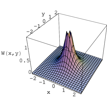
(a)$\;\nu=-0.2$

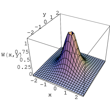
(b)$\;\nu=0.1$

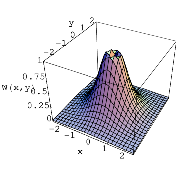
(c)$\;\nu=0.4$

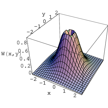
(d)$\;\nu=0.7$

Figure 1: The radial probability density of $s$-state of a two-dimensional quasi-free particle with PDM is $0$ at the origin, but has a maximum close to the origin. The radial probability density decays exponentially for large $\rho$. The parameters are $|E|=\frac{1}{2}$, and $\nu=-0.2,\,0.1,\,0.4,\,0.7$, respectively.

(a)$\;\nu=-0.2$

(b)$\;\nu=0.1$

(c)$\;\nu=0.4$

(d)$\;\nu=0.7$

Figure 2: The cut of the radial probability density of the $s$-state for a two-dimensional quasi-free particle with PDM shows that the maximum of the probability density deviates from he origin with $\nu$ increasing. The parameters are the same as those in Fig.1.

If $E=|E|>0$, we make the similar transformation as in Eq. (14), then the radial Schrödinger equation for $l=0$ and the mass function $\mu(\rho)=\rho^{\alpha}$ reads

$$z^{2}\frac{d^{2}\xi(z)}{dz^{2}}+z\frac{d\xi(z)}{dz}+(z^{2}-\nu^{2})\xi(z)=0.$$ (20)

Eq.(20) has two special solutions $J_{\nu}(z)$ and $Y_{\nu}(z)$ which are first and second kind of Bessel functions, respectivelymag . Considering of the asymptotic behavior of $J_{\nu}(z)$ and $Y_{\nu}(z)$ around the origin and large $|z|$ we have the solution of Eq.(20) to be of the form

$$\xi=CJ_{\nu}(z)+DY_{\nu}(z),$$ (21)

where $C$ and $D$ are constants. The radial eigenfunction for the positive energy is

$$u(\rho)=z^{\nu}(CJ_{\nu}(z)+DY_{\nu}(z)).$$ (22)

The related probability density function of the above eigenfunction does not possess of the property of localization near the origin.

III.2 Three-dimensional system

We use the same form of mass function $\mu(r)=r^{\alpha}$ as that for the two-dimensional system, then the radial Schrödinger equation for the three-dimensional quasi-free particle is

$$-\frac{1}{2}\frac{d^{2}u(r)}{dr^{2}}+\frac{1}{2}\frac{2-\alpha}{r}\frac{du(r)}{dr}+\frac{l(l+1)}{2r^{2}}u(r)=-|E|r^{\alpha}u(r),$$ (23)

where $u(r)$ is the radial wave function which has the relation to $R(r)$ in Eq.(5)

$$u(r)=\frac{R(r)}{r}.$$ (24)

For the state of $l=0$, Eq.(23) reads

$$\frac{d^{2}u(r)}{dr^{2}}+\frac{2-\alpha}{r}\frac{du(r)}{dr}=2|E|r^{\alpha}u(r).$$ (25)

Making the replacements of the following forms

$$z=\frac{2\sqrt{2|E|}}{\alpha+2}r^{(\alpha+2)/2},\;\nu=\frac{\alpha-1}{2+\alpha},\;u(\rho)=z^{\nu}\xi(z),$$ (26)

we will turn Eq.(25) into the standard modified Bessel equation as Eq.(15). Now, $\nu$ is restricted in the range $(-\frac{1}{2},\,1)$ due to $\alpha>0$.

Similar to the analysis of the two-dimensional system and with the requirement that $u$ is finite when $r$ is large, the general solution of Eq.(15) is

$$\xi=cK_{\nu}(z),$$ (27)

where $c$ is an arbitrary constant. The normalized solution of Eq.(25) is

$$u(r) =cz^{\nu}K_{\nu}(z)=\sqrt{\frac{\sin(\nu\pi)}{2\nu\pi^{2}}}\left[\frac{2}{3}(1-\nu)\right]^{\frac{1}{2}(1-2\nu)}\left(2|E|\right)^{\frac{1}{2}(1-\nu)}z^{\nu}K_{\nu}(z)$$ (28)

$$=\sqrt{\frac{8|E|\sin(\nu\pi)(1-\nu)}{3\nu\pi}}r^{\frac{\nu}{2(1-\nu)}}K_{\nu}(\frac{2}{3}(1-\nu)\sqrt{2|E|}r^{\frac{3}{2(1-\nu)}}).$$

The probability of finding the particle in the range $r$ to $r+dr$ is

$$W(r)\,dr= \int_{0}^{2\pi}d\theta\int_{0}^{\pi}\sin\varphi\,d\varphi\,r^{2}\,dr|\psi|^{2}$$ (29)

$$= \int_{0}^{2\pi}d\theta\int_{0}^{\pi}\sin\varphi\,d\varphi\,r^{2}\,dr|u(r)|^{2}|Y_{00}(\theta,\varphi)|^{2}=|u(r)|^{2}r^{2}\,dr$$

$$= \frac{8|E|\sin(\nu\pi)(1-\nu)}{3\nu\pi}r^{\frac{2-\nu}{1-\nu}}K_{\nu}^{2}(\frac{2}{3}(1-\nu)\sqrt{2|E|}r^{\frac{3}{2(1-\nu)}})\,dr.$$

For the three-dimensional system, the relationship between the probability density $W(r)$ and $r$ is similar to that for the two-dimensional system. There also exists localization of the wave function for the $s$ state around the origin.

Similar to the discussion for the two-dimensional system in the last subsection, the eigenfunction and the related probability density function for the positive energy in three dimensions have also no localization close the origin.

IV Conclusions and Discussions

In this article, we discussed the properties of the $s$-state of a quasi-free particle with PDM. When mass varies with radial coordinate $r$, it induces additional effective potential which may produce central attractive force and may cause the wave function of the $s$-state to localize around the origin. In $D$, except $D=1$, dimensional system with the mass of the particle being position-dependent, the localization appears, which contrasts sharply with the system of constant mass. We solve the radial Schrödinger equation to get the exact $s$-wave function for a specific mass function in two and three dimensions, respectively. Their corresponding probability densities and the related asymptotic behaviors are also analyzed, and the results are consistent with the general discussions.

There are many kinds of mass functions that are used in the investigation of the systems with PDM, but it is difficult to get the exact solutions of the radial Schrödinger equations for these mass functions in higher dimensional systems. So some numerical studies are required for the understanding of the properties of the systems with these mass functions.

References

- (1) R. E. Prange and S. M. Girvin, The Quantum Hall Effect, Springer-Verlag, 1990
- (2) K. Huang, Statistical Mechanics, 2nd., New York :John Wiley & Sons, 1987
- (3) J. M. Kosterlitz and D. J. Thouless 1973 J. Phys. C6:1181
- (4) S. Flügge, Practical Quantum Mechanics, Springer-Verlag,1974
- (5) M. V. Berry and A. M. Ozorio de Almeida 1973 J. Phys. A6:1451
- (6) M. A. Cirone, K. Rzażewski, W. P. Schleich, F. Straub and J. A. Wheeler 2001 Phys. Rev. A65:022101
- (7) I. Białynicki-Birula, M. A. Cirone, J. P. Dahl, M. Fedorov and W. P. Schleich 2002 Phys. Rev. Lett 89:060404
- (8) W. P. Schleich and J. P. Dahl 2002 Phys. Rev. A65:052109
- (9) J. Botero, M. A. Cirone, J. P. Dahl, F. Straub and W. P. Schleich 2003 Appl. Phys. B76:129
- (10) J. P. Dahl and W. P. Schleich 2002 Phys. Rev. A65:022109
- (11) I. Białynicki-Birula, M. A. Cirone, J. P. Dahl, R. F. O’Connell and W. P. Schleich 2002 J. Opt. B4:S393
- (12) M. A. Cirone, J. P. Dahl, M. Fedorov,D. Greenberger and W. P. Schleich 2002 J. Phys. B35:191
- (13) O. von Roos 1983 Phys. Rev. B27:7547
- (14) G. Bastard 1988 Wave Mechanics Applied to Semiconductor Heterostructure (Les Ulis Editions de Physique)
- (15) L. T. Serra and E. Lipparini 1997 Europhys. Lett. 40:667
- (16) M. Barranco, M. Pi, S. M. Gatica, E. S. Hernandez and J. Navarro 1997 Phys. Rev. B56: 8997
- (17) J. M. Levy-Leblond 1995 Phys. Rev. A52:1845
- (18) A. R. Plastino , M. Casas, F. Garcias and A. Plastino 1999 Phys. Rev. A60:4318
- (19) V. Milanovic, Z. Ikovic 1999 J. Phys. A: Maht. Gen. 32:7001
- (20) A. de Souza Dutra, C. A. S. Almeida 2000 Phys. Lett. A275:25
- (21) B. Gönül, B. Gönül, D. Tutcu and O. Özer 2002 Mod. Phys. Lett. A17:2057
- (22) B. Gönül, O. Özer, B. Gönül and F. Üzgün 2002 Mod. Phys. Lett. A17:2453
- (23) A. Alhaidari 2002 Phys. Rev. A66:042116
- (24) R. Koc and M. Koca 2003 J. Phys. A: Math. Gen. 36:8105
- (25) C. Quesne and V. M. Tkachuk 2003 J. Phys. A: Math. Gen. 36:10373
- (26) C. Quesne and V. M. Tkachuk 2004 J. Phys. A: Math. Gen. 37:10095
- (27) C. Quesne and V. M. Tkachuk 2004 J. Phys. A: Math. Gen. 37:4267
- (28) B. Bachi, A. Banerjee, C. Quesne and V. M. Tkachuk 2005 J. Phys. A: Math. Gen. 38:2929
- (29) C. Y. Cai, Z. Z. Ren and G. X. Ju 2005 Commun. Theor. Phys. 43:1019
- (30) M. Bander and C.Itzykson 1966 Rev. Mod. Phys. 38:330,346
- (31) M. M. Nieto 1979 Am. J. Phys. 47:1067
- (32) V. A. Kostelecky, M. M. Nieto and D. R. Truax 1985 Phys. Rev. D 32:2627
- (33) J. Avery 1993 J. Phys. Chem. 97:2406
- (34) G. Levai, B. Konya and Z. Papp 1998 J. Math. Phys. 39: 5811
- (35) G. Paz 2002 J. Phys. A 35:3727
- (36) W. Magnus, F. Oberhettingger and R. P. Soni, Formulas and Theorems for the Special Functions of Mathematical Physics, Springer-Verlag, 1966