We present an analytical expression for the response of a transient spectrum to a single-Cooper-pair box biased by a classical voltage and irradiated by a single-mode quantized field. The exact solution of the model is obtained, by means of which we analyze the analytic form of the fluorescence spectrum using the transitions among the dressed states of the system. An interesting relation between the fluorescence spectrum and the dynamical evolution is found when the initial field states are prepared in binomial states.

1 Introduction

For quantum information science and technologies, it is crucial to build the fundamental quantum logic gates [1]. Together with the basic single bit logic gates, the non-trivial two bit gates constitutes the fundamental blocks for the quantum network of quantum computing. The present lack of a current standard based on quantum devices has inspired several attempts to manipulate single electrons, or Cooper pairs, where the rate of particle transfer is controlled by an external frequency. Various superconducting nanocircuits have been proposed as quantum bits (qubits) for a quantum computer [2, 3]. In principle, any two-state quantum system works as a qubit, the fundamental unit of quantum information. However, only a few real physical systems have worked as qubits, because of requirements of a long coherent time and operability. Among various physical realizations, such as ions traps, QED cavities, quantum dots and NMR etc., superconductors with Josephson junctions offer one of the most promising platforms for realizing quantum computation [2, 3, 4, 5, 6].

The single-Cooper-pair transistor [7, 8], is composed of two ultrasmall tunnel junctions in series forming an island. Transport through the single-Cooper-pair transistor depends on the electrostatic energy required to charge the island, as in the single-electron transistor, and also on the Josephson coupling across the junctions. Cooper-pair boxes are one of the prominent candidates for qubits in a quantum computer. Recent experiments [9] have revealed quantum coherent oscillations in two CPBs coupled capacitively and demonstrated the feasibility of a conditional gate as well as creating macroscopic entangled states. Scalable quantum-computing schemes [9] have been proposed based on charge qubits. In architectures based on Josephson junctions coupled to resonators, the resonators store single qubit states, transfer states from one Josephson junction to another, entangle two or more Josephson junctions, and mediate two-qubit quantum logic. In effect, the resonators are the quantum computational analog of the classical memory and bus elements.

In this paper we deal with the problem of the interaction between a single-mode quantized field and a single-Cooper-pair box biased by a classical voltage. Despite the complexity of the problem, we obtain a quite simple master equation that is valid for arbitrary values of the Rabi frequency and the detuning. We apply the Fourier transform of the time averaged dipole-dipole correlation function to calculate the fluorescence spectrum, assuming that the electromagnetic field is initially in a binomial state. We find that the detuning changes considerably the shape of the resonance fluorescence spectrum and leads to novel spectral features. The organization of this paper is as follows: in section 2 we introduce the model and give exact expression for the unitary operator. In section 3 we employ the analytical results obtained in section 2 and by using the finite double-Fourier transform of the two-time field correlation function we find an analytical expression for the spectrum. Finally, we summarize the results in section 4.

2 The model

Several schemes have been proposed for implementing quantum computer hardware in solid state quantum electronics. These schemes use electric charge, magnetic flux, superconducting phase, electron spin, or nuclear spin as the information bearing degree of freedom [11]. In this paper, we consider an example of a realistic system, fabricated by the present day technology. We consider a superconducting box with a low-capacitance Josephson junction (with the capacitance $C_{J}$ and Josephson energy $E_{J}$), biased by a classical voltage source $V_{g}$ through a gate capacitance $C_{g}$ and placed inside a single-mode microwave cavity. Suppose the gate capacitance is screened from the quantized radiation field, then the junction-field Hamiltonian, in the interaction picture, can be written as [12]

$$\hat{H}_{in}=\frac{(Q-C_{g}V_{g}-C_{J}V)^{2}}{2(C_{g}+C_{J})}-E_{J}\cos\phi.$$ (1)

where the relevant conjugate variables are the charge $Q=2Ne$ on the island (where $N$  is the number of Cooper-pairs) and the phase difference $\phi$ across the junction. The radiation field is to produce an alternating electric field of the same frequency across the junction, and $V$ is the effective voltage difference produced by the microwave across the junction. We assume that the dimension of the device is much smaller than the wavelength of the applied quantized microwave (which is a realistic assumption), so the spatial variation in the electric field is negligible. We also assume that the field is linearly polarized, and is taken perpendicular to the plane of electrodes, then $V$ may be written down as [13]

$$V=i\left(\frac{\hslash\omega}{2C_{F}}\right)\left(\hat{\psi}-\hat{\psi}^{\dagger}\right),$$ (2)

where $\hat{\psi}^{\dagger}$ and $\hat{\psi}$ are the creation and annihilation operators of the microwave with frequency $\omega$. $C_{F}$ is the capacitance parameter, which depends on the thickness of the junction, the relative dielectric constant of the thin insulating barrier, and the dimension of the cavity. In this paper we consider the case where the charging energy with scale

$$E_{c}=\frac{e^{2}}{2}\left(C_{g}+C_{J}\right),$$

dominates over the Josephson coupling energy $E_{{}_{J}}$, and concentrate on the value $Vg=\frac{e}{C_{g}}$, so that only the low-energy charge states $N=0$ and $N=1$ are relevant. In this case the Hamiltonian in a basis of the charge state $\left|\downarrow\right\rangle$ and $\left|\uparrow\right\rangle$ reduces to a two-state form. In a spin-$1/2$ language [15]

$$\hat{H}_{in}=E_{c}\left(1+\frac{C_{J}^{2}}{e^{2}}V^{2}\right)-\frac{1}{2}E_{J}\sigma_{x}+2E_{c}\frac{C_{J}}{e}V\sigma_{z}.$$ (3)

where $\sigma_{x}$ and $\sigma_{z}$ are the Pauli matrices in the pseudo-spin basis.

The time development of the state vector $|\psi(t)\rangle$ of the system is postulated to be determined by Schrödinger equation

$$i\hbar\frac{d}{dt}|\psi(t)\rangle=\widehat{H}_{in}|\psi(t)\rangle.$$ (4)

The solution of equation (4) can be written as $|\psi(t)\rangle=\hat{U}_{t}|\psi(0)\rangle,$ where $\hat{U}_{t}$ is a time evolution operator which depends on the Hamiltonian of the system. Since $|\psi(0)\rangle$ is arbitrary, the time evolution operator obeys $i\hbar dU_{t}/dt=\widehat{H}_{in}U_{t}.$ Integrating this equation, gives $U_{t}$ $\equiv\exp\left(\frac{-i}{\hbar}\int\hat{H}_{in}dt\right).$ If the system is conservative and $\hat{H}_{in}$ is explicitly independent of time, then $U_{t}$ reduces to $U_{t}$ $\equiv\exp\left(\frac{-i}{\hbar}\hat{H}_{in}t\right).$

One may, also, assume that the two eigenstates $|\Phi_{1,2}^{(n)}\rangle$ are known, along with their corresponding eigenenergies $\Upsilon_{\pm}^{(n)}.$Then we can write the time evolution operator as

$$\hat{U}_{t}=\sum\limits_{n=0}^{\infty}\left\{\exp(-i\Upsilon_{+}^{(n)}t)|\Phi_{1}^{(n)}\rangle\langle\Phi_{1}^{(n)}|\right.\left.+\exp(-i\Upsilon_{-}^{(n)}t)|\Phi_{2}^{(n)}\rangle\langle\Phi_{2}^{(n)}|\right\}.$$ (5)

In order to find explicit forms of the eigenvalues and eigenvectors, we consider the weak quantized radiation field and then we can neglect the term containing $V^{2}$ in equation (3) and using the rotating wave approximations we obtain

$$\Upsilon_{\pm}^{(n)} = \omega(n+1/2)\pm\mu_{n},$$

$$\mu_{n} = \sqrt{\frac{\Delta^{2}}{4}+\frac{e^{2}C_{J}^{2}}{2(C_{J}+C_{g})^{2}}\times{\frac{\omega}{2\hslash C_{J}}}\times(n+1)}.$$ (6)

We denote by $\Delta=E_{J}-\omega$ the detuning between the Josephson energy and cavity field frequency. $|\Phi_{1,2}^{(n)}\rangle$ are given by

$$|\Phi_{1}^{(n)}\rangle = \cos\left(\tan^{-1}\left(\frac{(C_{J}+C_{g})\left(-\Delta+2\mu_{n}\right)}{eC_{J}\sqrt{(n+1)}}\sqrt{\frac{2\hslash C_{J}}{\omega}}\right)\right)|n,\uparrow\rangle$$ (7)

$$+\sin\left(\tan^{-1}\left(\frac{(C_{J}+C_{g})\left(-\Delta+2\mu_{n}\right)}{eC_{J}\sqrt{(n+1)}}\sqrt{\frac{2\hslash C_{J}}{\omega}}\right)\right)|n+1,\downarrow\rangle{\Large,}$$

$$|\Phi_{2}^{(n)}\rangle = \sin\left(\tan^{-1}\left(\frac{(C_{J}+C_{g})\left(-\Delta+2\mu_{n}\right)}{eC_{J}\sqrt{(n+1)}}\sqrt{\frac{2\hslash C_{J}}{\omega}}\right)\right)|n,\uparrow\rangle$$ (8)

$$-\cos\left(\tan^{-1}\left(\frac{(C_{J}+C_{g})\left(-\Delta+2\mu_{n}\right)}{eC_{J}\sqrt{(n+1)}}\sqrt{\frac{2\hslash C_{J}}{\omega}}\right)\right)|n+1,\downarrow\rangle{\Large.}$$

We devote the next section to investigate the general structure of the dipole-dipole correlation function in terms of the eigenstates and eigenvalues of the system, and evaluate the fluorescence spectrum for input binomial states.

3 The transient spectrum

For the calculation of the spectrum, we consider the time evolution of the off-diagonal density matrix elements of the field while the diagonal density matrix elements remain stationary. In this section we derive the physical transient spectrum $S(\nu)$ by calculating the Fourier transform of the time averaged dipole-dipole correlation function $\langle\sigma_{+}(t+\tau)\sigma_{-}(t)\rangle$, weighted by the detector response function $\langle\psi(0)|\sigma_{+}(t+\tau)\sigma_{-}(t)|\psi(0)\rangle$ where $|\psi(0)\rangle$ is the initial state of the considered system. Then, the transient spectrum is given by the expression [14]

$$S(\nu)=Re\left(\int\limits_{0}^{\infty}d\tau\exp[-i\nu\tau-\gamma\tau]\overline{\langle\psi(0)|\sigma_{+}(t+\tau)\sigma_{-}(t)|\psi(0)\rangle}d\tau\right),$$ (9)

where $\gamma$ is the detector width and $\nu$ is the spectrum frequency.

Using equations (5)-(8), the time evolution of the states can be expressed as

$$\hat{U}_{t}|n,e\rangle = A(n,t)|n,e\rangle+B(n,t)|n+k,g\rangle,$$

$$\hat{U}_{t}|n,g\rangle = A(n-k,t)|n,g\rangle+B(n-k,t)|n-k,e\rangle,$$ (10)

where

$$A(n,t) = \sin^{2}\left(\tan^{-1}\left(\frac{(C_{J}+C_{g})\left(-\Delta+2\mu_{n}\right)}{eC_{J}\sqrt{(n+1)}}\sqrt{\frac{2\hslash C_{J}}{\omega}}\right)\right)\exp\left(-it\Upsilon_{-}^{(n)}\right)$$ (11)

$$+\cos^{2}\left(\tan^{-1}\left(\frac{(C_{J}+C_{g})\left(-\Delta+2\mu_{n}\right)}{eC_{J}\sqrt{(n+1)}}\sqrt{\frac{2\hslash C_{J}}{\omega}}\right)\right)\exp\left(-it\Upsilon_{+}^{(n)}\right),$$

$$B(n,t) = \frac{1}{2}\sin 2\left(\tan^{-1}\left(\frac{(C_{J}+C_{g})\left(-\Delta+2\mu_{n}\right)}{eC_{J}\sqrt{(n+1)}}\sqrt{\frac{2\hslash C_{J}}{\omega}}\right)\right)$$ (12)

$$\times\biggl{[}\exp\left(-it\Upsilon_{+}^{(n)}\right)-\exp\left(-it\Upsilon_{-}^{(n)}\right)\biggr{]}.$$

By using the above equations, the correlation function $\langle\hat{\sigma}_{+}(t+\tau)\hat{\sigma}_{-}(t)\rangle$ can be evaluated in terms of the coefficients $A(n,t)$ and $B(n,t),$ as follows (the box initially prepared in the excited state i.e. the initial state of the system is assumed to be $\left|\psi(0)\right\rangle=\sum\limits_{n=0}^{M}\beta_{n}^{M}(\eta)\left|n,e\right\rangle,$ where $\beta_{n}^{M}(\eta)$ will be defined latter)

$$\langle\hat{\sigma}_{+}(t+\tau)\hat{\sigma}_{-}(t)\rangle = \sum\limits_{n=0}^{\infty}\left(\beta_{n}^{M}\right)^{2}\langle n,e|\hat{\sigma}_{+}(t+\tau)\hat{\sigma}_{-}(t)|n,e\rangle$$ (13)

$$= \sum\limits_{n=0}^{\infty}\left(\beta_{n}^{M}\right)^{2}A(n,t)A(n-k,\tau)A^{\ast}(n,t-\tau).$$

The Fourier transform of the time averaged dipole-dipole correlation, which is directly related to the fluorescence spectrum with the identification of $\gamma$ as the width associated with the detector [14]. After carrying out the various operations we get

$$S(\nu) = \left(\beta_{0}^{M}\right)^{2}\left(\frac{\gamma\sin^{4}\theta_{0}}{\gamma^{2}+(\nu-\Upsilon_{0}^{+})^{2}}+\frac{\gamma\cos^{4}\theta_{0}}{\gamma^{2}+(\nu-\Upsilon_{0}^{-})^{2}}\right)$$ (14)

$$+\sum\limits_{n=1}^{\infty}\left(\beta_{n}^{M}\right)^{2}{\Huge[}\frac{\gamma\sin^{4}\theta_{n}\cos^{2}\theta_{n-k}}{\gamma^{2}+(\nu+\Upsilon_{n-k}^{+}-\Upsilon_{n}^{+})^{2}}+\frac{\gamma\sin^{4}\theta_{n}\sin^{2}\theta_{n-k}}{\gamma^{2}+(\nu+\Upsilon_{n-k}^{-}-\Upsilon_{n}^{+})^{2}}$$

$$+\frac{\gamma\cos^{4}\theta_{n}\cos^{2}\theta_{n-k}}{\gamma^{2}+(\nu+\Upsilon_{n-k}^{+}-\Upsilon_{n}^{-})^{2}}+\frac{\gamma\cos^{4}\theta_{n}\sin^{2}\theta_{n-k}}{\gamma^{2}+(\nu+\Upsilon_{n-k}^{-}-\Upsilon_{n}^{-})^{2}}{\Huge],}$$

where $\left(\beta_{n}^{M}\right)^{2}$ is the initial photon number distribution and $\theta_{n}$ is

$$\theta_{n}=\tan^{-1}\left(\frac{(C_{J}+C_{g})\left(-\Delta+2\mu_{n}\right)}{eC_{J}\sqrt{(n+1)}}\sqrt{\frac{2\hslash C_{J}}{\omega}}\right).$$

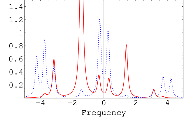
Figure 4: The same as in figure 2 but $\Delta=g$.

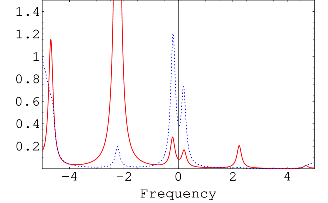
Figure 5: The same as in figure 2 but $\Delta=2g$.

Thus the time averaged spectrum consists of resonant structures which arise from transitions among different dressed states. The final structure of the time averaged spectrum will depend on the form of the input photon distribution. As the cavity field starts to interact with the Cooper pair the initial photon number distribution starts to change. Due to the quantum interference between component states the oscillations in the cavity field become to be composed of two component states. The situation that has just been described is depicted in figures 1-5.

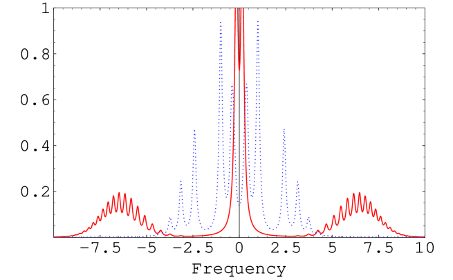
Figure 1: The evolution of the function $S(\upsilon)$ in a perfect cavity as a function of ($\upsilon-\omega)/\lambda$ for an input binomial state, with the $\eta=0,M\rightarrow\infty(i.e.\eta M=|\alpha|^{2}$ where $|\alpha|^{2}=10$ (solid line) and $|\alpha|=1$( dotted line). Calculations assume detector width $\gamma=0.1g$, and the detuning parameter $\Delta$ has zero value.

In figure 1 we discuss the spectrum for the situation of a coherent field with $\Delta=0$. We show the evolution of this spectrum $S(\upsilon)$ as a function of ($\upsilon-\omega)/\lambda$ where $\lambda=\frac{eC_{J}}{2(C_{J}+C_{g})}\sqrt{\frac{\omega}{2\hslash C_{J}}}$. We consider the initial state of the field is a binomial state. The binomial states which has been introduced by Stoler, Saleh and Teich in [2], interpolate between the most nonclassical states, such as number states and coherent states, and reduce to them in two different limits. Some of their properties [2, 3, 4], methods of generation [2, 3, 5], as well as their interaction with atoms [6], have been investigated in the literature. The binomial state is defined as a linear superposition of number states in an $M-$dimensional subspace

$$\left|\eta,M\right\rangle=\sum\limits_{n=0}^{M}\beta_{n}^{M}(\eta)\left|n\right\rangle,$$ (15)

where the state $\left|n\right\rangle$ is the number state of the field mode, $\eta$ is a complex number with the absolute value between $0$ and $1$, $M$ is a positive integer, and

$$\beta_{n}^{M}(\eta)=\sqrt{\left(\begin{array}[]{c}M\\ n\end{array}\right)\left(\eta^{n}+(1-\eta)^{n-M}\right)}.$$ (16)

The name binomial state comes from the fact that their photon distribution is simply a binomial distribution with probability $\eta$. The binomial state is a linear combination of $M+1$ number states with coefficients chosen such that the photon-counting probability distribution is binomial with mean photon $M$. This state can produce, under certain choices of the parameters $\eta$ and $M$, the number state $\left|M\right\rangle$, the vacuum state $\left|0\right\rangle$ and the coherent state. When $\eta\rightarrow 0,$ $M\rightarrow\infty$  with $\eta M=\alpha^{2}$ fixed ($\alpha$ real constant), $\left|\eta,M\right\rangle$ reduces to the coherent states which correspond to the Poisson distribution. Here we consider $\eta=0,M\rightarrow\infty$ and $|\alpha|^{2}=10$ (solid line) and $|\alpha|=1$ (dotted line). Calculations assume that the detector width $\gamma=0.1\lambda$, and the detuning parameter $\Delta$ has zero value. The slit is adjusted so that the light is collected from Cooper-pair box which have been in the field for times ranging from 0 up to 7. From an initially broad featureless spectrum, the central peak and the sidebands emerge rather quickly. As the observation region is lengthened, all the components get taller and narrower. Then for about ($\upsilon-\omega)\approx\pm 9\lambda$, the transient spectrum has narrowed enough and tends to zero. In the limit of a very large mean photon number and at exactly resonant field, it is possible to simplify the expression for the spectrum $S(\nu)$ and illustrate explicitly the manner in which the sidebands and the central peaks narrow with increasing ($\upsilon-\omega)$.

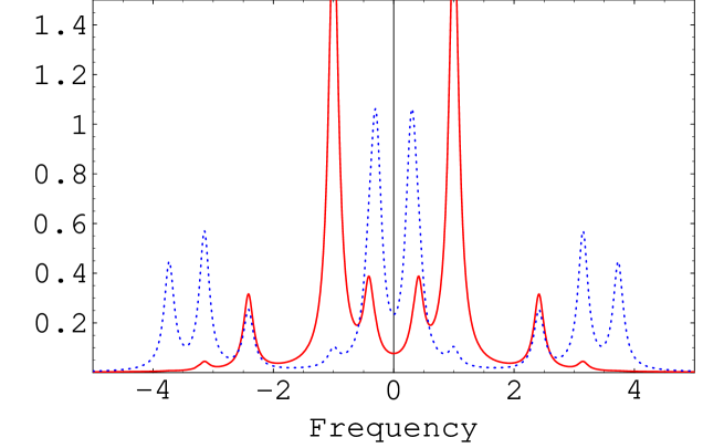
Figure 2: The evolution of the function $S(\upsilon)$ in a perfect cavity as a function of ($\upsilon-\omega)/\lambda$ for an input binomial state, with $M=3$, $\eta=0.7$ for (solid line) and $\eta=0.1$ for (dotted line). Calculations assume that, the detector width $\gamma=0.1g$, and the detuning parameter $\Delta$ has zero value.

It would be of interest to pay attention to the physical transient spectrum for binomial states. In order to do that, we use different values of both $\eta$ and $M$ (say $M=3$ and $\eta=0.7,$ $0.1$). This basis is overcomplete and many states in the Hilbert space can be expanded in it. The behaviors of $S(\nu)$ is notably different from those observed in the coherent state case. Indeed, in the fully connected system considered here, $S(\nu)$ is extremum at $\pm 1(\pm 0.4)$ when $\eta=0.7(0.1)$ whereas in the coherent state case, figure 1, $S(\nu)$ is extremum at $\approx 0$. In addition, the scaling behavior of the spectrum and of its derivative are different in both cases. Therefore, when speaking about the physical transient spectrum sensitivity achieved with different frequencies, it is necessary to specify the kind of initial state of the field.

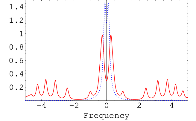
Figure 3: The same as in figure 2 but $M=30$.

Our aim is now to evaluate the response of the physical transient spectrum due to the mean photon $M$.  It is interesting to note that in a large value of $M,$ we observe a similar behavior to that obtained in the coherent state, see figure 3. Now, we would like to shed some light on the spectrum behavior when the detuning differs from zero. The transient spectrum under these conditions can be asymmetric and ultimately the central component and one of the Rabi sidebands can vanish despite the fact that the quadrature-noise spectrum exhibits a significant amount of noise at these frequencies. The asymmetry arises from the stimulated emission induced between the dressed states by the binomial field.

These asymmetries consist of an enhanced sideband on the atomic resonance frequency side of the central peak and more pronounced oscillations between the central peak and the enhanced sideband than on the opposite side of the central peak. Also, we observe a slight displacement in the location of the central maximum from the applied field frequency toward the atomic frequency. One can see that the large value of the detuning parameter gives a disappearance of one peak and large displacement in the location of the maximum value of the spectrum.

We can conclude that the effect of the detuning on the spectrum of the emitted light is twofold. The first effect is the shift of the spectrum to the left or to the right depending on the sign of $\Delta$. The second effect is the dependence of the amplitude of the peaks on $\Delta$. This dependence leads to the fact that, in the far off-resonance limit, only one peak survives.

Finally we may point out that the present lack of a current standard based on quantum devices has inspired several attempts to manipulate single electrons, or Cooper pairs, where the rate of particle transfer is controlled by an external frequency [16]. In the experiments described in [17] a long array of Josephson junctions with an external signal applied to a gate, which is capacitively coupled to the middle of the array has been used. Theoretically many systems can act as a qubit, but the realization of it is difficult. Nakamura et al. [18] have shown in their experiments with single Cooper pair box, that in a kind of metallic island structures the oscillations between eigenstates of the system last at least a few nanoseconds. The states are characterized by the number of Cooper pairs in the box and (quantum) manipulation of this number is of basic importance for the production of viable qubits. This might be a very important issue when thinking of the limitations on the preparation and read-out of the states.

4 Conclusion

We have analyzed the physical transient spectrum of a single Cooper-pair box, which is biased by a classical voltage and irradiated by a single-mode quantized field. We emphasize the fact that the proper expression for the emission spectrum which is derived in this paper can be measured in a realistic experiment. This spectrum has been obtained not only as a function of the atomic and field parameters, but also as a function of $\gamma$ which is available to the experimenter ($\gamma$ the width associated with the detector). Thus it correctly incorporates the possible effects of a finite observation interval, observations made close to the point where the interaction was turned on, and arbitrary initial conditions for the Cooper pair box at the start. Among the reasons for the interest in considering nonclassical effects of the binomial states, we may mention the following reasons: the experimental work shows that nonclassical effects serve as a test of the quantum nature of light and nonclassical behavior of light is usually connected with a noise reduction below a standard limit (e.g. the shotnoise limit). In particular, we have explored the influence of various parameters of the system on the emission spectrum of the output field statistics. We have used the finite double-Fourier transform of the two-time field correlation function to find an analytical expression for the spectrum. The spectrum in the cavity for the initial binomial states is studied. Such systems are potentially interesting for their ability to process information in a novel way and might find application in models of quantum logic gates. The phenomenon of oscillations in the field spectrum has been shown. It is observed that the symmetry shown in the resonant case for the spectra is no longer present once the detuning is added.

References

- [1] F. W. Strauch, P.R. Johnson, A. J. Dragt, C. J. Lobb, J. R. Anderson, and F. C. Wellstood, Phys. Rev. Lett. 91, 167005 (2003).
- [2] A. J. Berkley, H. Xu, R. C. Ramos, M. A. Gubrud, F. W. Strauch, P. R. Johnson, J. R. Anderson, A. J. Dragt, C. J. Lobb, and F. C. Wellstood, Science 300, 1548 (2003)
- [3] L. F.Wei and F. Nori, Europhys. Lett. 67, 1004 (2004)
- [4] F. Plastina and G. Falci, Phys. Rev. B 67, 224514 (2003).
- [5] D. V. Averin and C. Bruder, Phys. Rev. Lett. 91, 057003 (2003).
- [6] A. Wallraff, D. I. Schuster, A. Blais, L. Frunzio, R.-S. Huang, J. Majer, S. Kumar, S. M. Girvin and R. J. Schoelkopf, Nature (London) 431, 162 (2004)
- [7] T. A. Fulton et al.: Phys. Rev. Lett. 63, 1307 (1989).
- [8] Y. Makhlin, G. Schön, and A. Shnirman, Rev. Mod. Phys. 73, 357 (2001).
- [9] Y. A. Pashkin, T. Yamamoto, O. Astafiev, Y. Nakamura, D. V. Averin and J. S. Tsai, Nature 421, 823 (2003).
- [10] J. Q. You, J. S. Tsai, and F. Nori, Phys. Rev. Lett. 89, 197902 (2002).
- [11] Y. Makhlin, G.Schön, and A. Shnirman, Nature 398, 305 (1999); 8. L.B. Ioffe, V.B. Geshkenbein, M.V. Feigelman, A.L. Fauchere, G. Blatter, Nature 398, 679 (1999); B. Kane, Nature, 393, 133 (1998); D. Loss, D. DiVincenzo, Phys. Rev. A 57, 120 (1998).
- [12] R. Migliore, A. Messina and A. Napoli, Eur. Phys. J. B 13, 585 (2000); 22, 111 (2001)
- [13] M. Zhang, J. Zpu and B. Shao, Int. J. Mod. Phys. B 16, 4767 (2002)
- [14] J. H. Eberly and K. Wodkiewicz, J. Opt. Soc. Am. 67, 1252 (1977); G. S. Agarwal and R. R. Puri, Phys. Rev. A 33, 1757 (1986); V. Buzek, I Jex, J. Mod. Opt. 38, 987 (1991).
- [15] W. Krech and T. Wagner, Phys. Lett. A 275, 159 (2000).
- [16] M. Keller, J. M. Martinis, N. M. Zimmerman and A. H. Steinbach, Appl. Phys. Lett., 69, 1804, (1996).
- [17] M. Watanabe and D. B. Haviland, Phys. Rev. B 67, 094505 (2003); Coulomb blockade of Cooper pair tunneling in one dimensional Josephson junction arrays, K. Andersson, Ph. D. Thesis, Nanostructure Physics, KTH- The Royal Institute of Technology, Stockholm, Sweden 2002
- [18] Y. Nakamura, Yu. A Pashkin, and J. S. Tsai, Nature 398, 786 (1999).