Vanishing of electron pair recession at central impact

Abstract

Identity of electrons leads to description of their states by symmetrical or anti-symmetrical combination of free coherent states.

Due to the coordinate uncertainty potential energy of the Coulomb repulsing is limited from above and so when energy of electrons is large enough, electrons go through each other, without noticing one another.

We show existence of set of coherent states for which wave packages recession vanish - electrons remain close regardless of Coulomb repulsion.

1 Introduction

Taking into consideration the identity of electrons we describe their state by symmetrical or anti-symmetrical combination of free coherent states npyt ; sag ; pfff ; vacjpued . These states have a lot of essentially quantum pecularities such as entanglement gafi ; lgz ; llv ; bekvt .

Due to the coordinate uncertainty potential energy of the coulomb repulsing is limited from above. That is why two types of classical interpretation of electron interaction are possible:

• Classical scattering of an electron on another one. Electrons approach a certain distance, but due to the Coulomb repulsion they scatter in opposite directions.

• If energy of electrons is large enough, electrons go through each other, without noticing one another.

Two types of classic description of results of an impact take place for electrons with parallel and with anti-parallel spins as well.

In these two cases, due to recession of centers of packages of waves the entanglement of the state (both spatial and spin) remains constant. For the case of antiparallel mutual orientation of electron spins there is a certain range of relative momentum values at which recession of the centers of wave packages vanishes. Instead, spreading of wave packages takes place. The observed characteristic of the state is the quadrupole moment of the electric field produced by the pair of charges. In this case the spatial entanglement of the states vanishes simultaneously with packages spreading, in contrast to spin entanglement. Vanishing of recession makes evidence of the fact, that electrons are in the almost identical states long enough.

Will examine the pair of coherent electrons in the center-of-mass system, $r_{1}=\frac{R}{2}+r$, $r_{2}=\frac{R}{2}-r$, $p_{1}=\frac{P}{2}+p$, $p_{2}=\frac{P}{2}-p$. The Hamiltonian of this system is:

$$H=\frac{p_{1}^{2}}{2m}+\frac{p_{2}^{2}}{2m}+\frac{e_{0}^{2}}{\left|\vec{r}_{1}-\vec{r}_{2}\right|}=\frac{P^{2}}{4m}+\frac{p^{2}}{m}+\frac{e_{0}^{2}}{\left|\vec{r}_{1}-\vec{r}_{2}\right|}.$$ (1)

Hamiltonian of coherent electron pair is divided on Hamiltonian of free motion of center of mass of electron pair $H_{c}=\frac{\vec{P}^{2}}{4m}$ and Hamiltonian of relative motion

$$H_{r}=\frac{\vec{p}^{2}}{m}+\frac{e_{0}^{2}}{\left|\vec{r}\right|},$$ (2)

which is similar to the Hamiltonian of electron in the atom of hydrogen.

2 Wave function of coherent electron pair

Studying the electromagnetic field of coherent electron, (and also electromagnetic field of coherent electron pair), we deal with the problem on effect of coordinate and momentum uncertainties of free particle. Plane wave is not good instrument for description of the coherent electron state, because a flat wave is characterized a zero momentum uncertainty, and coordinate uncertainty tends to infinity. The same concerns to the functions, localized in space, that look like: $\delta(x-x_{0}(t))$. That is why we consider the wave function of coherent electron as Gaussian superposition of plane waves. Such kinds of probability distribution are characterized by the coordinate and momentum uncertainties $\sigma_{x}$ and$\sigma_{p}$. For the free particle, momentum uncertainty is constant,$\sigma_{p}=const$, but coordinate uncertainty depends on time.

2.1 Wave function of single coherent electron

Taking into consideration the aforesaid, we can write the wave function of coherent electron:

$$\Psi(\vec{r},\vec{r}_{0},\vec{p}_{0})=\frac{1}{\left({\sqrt{\sigma\sqrt{2\pi(1+\omega^{2}(t-t_{0})^{2})}}}\right)^{3}}\exp\left({-\frac{\left({\vec{r}-\vec{r}_{0}-\frac{\vec{p}_{0}}{m}(t-t_{0})}\right)^{2}}{4\sigma^{2}(1+\omega^{2}(t-t_{0})^{2})}+i\frac{\vec{p}_{0}\vec{r}}{\hbar}}\right),$$ (3)

where $\sigma$ is coordinate uncertainty, $r_{0}$- an average value of the coordinate, $p_{0}$- an average value of the momentum, $t_{0}$- is a culmination moment (moment of time, when correlation between the coordinate and momentum is absent), $m$- electron mass. Taking into consideration the uncertainty relation, which takes a minimum value in the moment of culmination, we can write down:

$$\sigma_{x}=\frac{\hbar}{2\sigma_{p}}\sqrt{1+\omega^{2}\left({t-t_{0}}\right)^{2}}$$ (4)

whence $\sigma_{r}\sigma_{p}=\frac{\hbar}{2}\sqrt{1+\omega^{2}\left({t-t_{0}}\right)^{2}}$. In the moment of culmination this expression takes a minimum value $\sigma_{r}\sigma_{p}=\hbar/2.$

As it is obvious from (4), the dependence of the wave package on time provides package spreading with time.

The kinetic energy of coherent electron:

$$T=\frac{p_{0}^{2}}{2m}+\frac{3\hbar}{4\sigma^{2}m},$$ (5)

where the first item describes the energy of quasi-classical motion of wave package center, the second item is conditioned by momentum uncertainty.

2.2 1. 2. Wave function of coherent electron pair

Wave function of coherent electron pair is an anti-symmetrical (in the case of parallel mutual spin orientation) or symmetrical (in the case of anti-parallel mutual spin orientation) combinations of wave functions of every electron (according to Pauli principle):

$$\Psi(\vec{r}_{1},\vec{r}_{2})=\frac{\Psi_{1}(\vec{r}_{2})\Psi_{2}(\vec{r}_{1})\pm\Psi_{1}(\vec{r}_{1})\Psi_{2}(\vec{r}_{2})}{\sqrt{1\pm N^{2}}}.$$ (6)

$N$ is an overlapping integral, which is defined is such a way:

$$N=\int{\Psi_{1}^{\ast}(r)}\Psi_{2}(r)d^{3}r=\left\langle{\Psi_{1}(r)}\mathrel{\left|{\vphantom{{\Psi_{1}(r)}{\Psi_{2}(r)}}}\right.\kern-1.2pt}{\Psi_{2}(r)}\right\rangle.$$ (7)

Overlapping integral is not equal to zero because wave functions are not orthogonal.

In the center-of-mass system average values of coordinate sum and momentum sum are equal to zero.

The parameters $\vec{r}_{0}$ and $\vec{p}_{0}$ have to take values of relative coordinate and relative momentum correspondingly. But these parameters should not be considered as average values of coordinate and momentum, because these values are equal to zero due to identity of electrons.

We consider coherent electron pair at $t=t_{0}$. The wave function is:

$$\begin{array}[]{l}\Psi(\vec{r}_{1},\vec{r}_{2})=\frac{1}{\sqrt{1\pm N^{2}}}\frac{1}{\left({\sigma\sqrt{2\pi}}\right)^{3}}\cdot\\ \cdot\left[{\exp\left({-\frac{\left({\vec{r}_{1}-\vec{r}_{0}}\right)^{2}}{4\sigma^{2}}-\frac{\left({\vec{r}_{2}+\vec{r}_{0}}\right)^{2}}{4\sigma^{2}}+i\frac{\vec{p}_{0}(\vec{r}_{1}-\vec{r}_{2})}{\hbar}}\right)}\right.\\ \pm\left.{\exp\left({-\frac{\left({\vec{r}_{2}-\vec{r}_{0}}\right)^{2}}{4\sigma^{2}}-\frac{\left({\vec{r}_{1}+\vec{r}_{0}}\right)^{2}}{4\sigma^{2}}+i\frac{\vec{p}_{0}(\vec{r}_{1}-\vec{r}_{2})}{\hbar}}\right)}\right]\\ \end{array}$$ (8)

Taking into consideration the wave function, the average of 2 is hnat :

$$\begin{array}[]{l}\left\langle H\right\rangle=\frac{p_{0}^{2}}{m}+\frac{3\sigma^{2}}{m}+\frac{\sigma^{2}\left|{\frac{2\sigma}{\hbar}r_{0}+\frac{i}{\sigma}p_{0}}\right|^{2}\exp\left({-\left|{\frac{2\sigma}{\hbar}r_{0}+\frac{i}{\sigma}p_{0}}\right|^{2}}\right)}{m\left({1+\exp\left({-\left|{\frac{2\sigma}{\hbar}r_{0}+\frac{i}{\sigma}p_{0}}\right|^{2}}\right)}\right)}\\ +e^{2}\frac{\frac{1}{\left|R\right|}erf\left({\frac{\sigma\left|R\right|}{\hbar\sqrt{1+\omega^{2}t^{2}}}}\right)-\frac{i}{\left|L\right|}erf\left({\frac{\sigma\left|L\right|}{\hbar\sqrt{1+\omega^{2}t^{2}}}}\right)\left|J\right|^{2}}{1+\left|J\right|^{2}}\end{array}$$ (9)

where $\left|R\right|=\frac{1}{2}\frac{1}{r(t)+\frac{t}{m}p(t)}$, $\left|L\right|=\frac{\hbar}{\sigma^{2}}\vec{p}(t)-2\omega t\vec{r}(t)$, $\left|J\right|^{2}=\exp(\left({-\left|{\frac{2\sigma}{\hbar}r(t)+\frac{i}{2}p(t)}\right|}\right)$ The average value of Hamiltonian of coherent electron pair depends on time. This dependence is determined by the fact that correlation between relative coordinate and relative momentum is absent in the initial moment of time only (moment of culmination).

3 Equations of motion

Using the method of integration by trajectories, Klauder has proved that one can obtain classical Hamiltonian equations of motion considering the average value of quantum system Hamiltonian as the Hamiltonian of classical system kla .

These equations go to classic equations of free motion of center of mass and equations of relative motion

$$\frac{d\vec{p}}{dt}=-\frac{\partial\left\langle H\right\rangle}{\partial\vec{r}},\frac{d\vec{r}}{dt}=\frac{\partial\left\langle H\right\rangle}{\partial\vec{p}}$$ (10)

Thus, in the Hamilton equations one should use relative coordinate and momentum. Equations of motion:

$$\frac{dp}{dt}=-\frac{\partial E}{\partial r}\quad,\quad\frac{dr}{dt}=\frac{\partial E}{\partial p},$$ (11)

where $E=\left\langle H\right\rangle$.

The average value of Hamiltonian of coherent electron pair depends on time. This dependence is determined by the fact that correlation between relative coordinate and relative momentum is absent in the initial moment of time only (moment of culmination).

The average value of energy of the system depends on time. This dependence is determined by the special quantum properties, first of all, by the effect of relative coordinate and momentum uncertainties. Even if the average values of coordinate and momentum are equal to zero, the average value of Hamiltonian depends on time due to spreading of wave package.

4 Central impact of coherent electrons

4.1 Quasi-classical model of the central impact

Due to the coordinate uncertainty potential energy of the coulomb repulsing is limited from above. That is why two types of classical interpretation of electron interaction are possible.

1. Scattering (same to the classical one) of an electron on another one. Electrons approach a certain distance, but due to the Coulomb repulsion they scatter in opposite directions (classical-like).

2. If energy of electrons is large enough, electrons go through each other, without noticing one another (tunneling-like).

Taking into consideration the principle of identity we find these two cases to be physically indistinguishable. We can not distinguish, which electron goes in certain direction. We can not find, whether they continue motion in the same directions, as before the impact (it means electrons fly over through each other), or in the opposite directions (it means, Coulomb repulsion took place).

We can calculate time $t$ electrons need to return to an initial distance. The traveltime differs according to the type of impact.

In classical approach to consideration of forward scattering, the falling electron stops, and the electron, which is the target, after scattering goes with the same speed the falling electron has had before scattering. Taking into consideration the principle of identity, we can not distinguish between the falling electron and the target electron. At the same time it is supposed, that Coulomb interaction between electrons remains and the potential interaction energy tends to infinity.

Dependence of traveltime on initial momentum is shown in figure 1.

Studying the central impact of coherent electrons, we can outline two types of traveltime behavior. For the first traveltime is definite at the any value of relative momentum. It takes place for the electrons with parallel mutual spin orientation, and the special case, for the electrons with anti-parallel mutual spin orientation as well, except the electrons, which have the relative momentum in the certain range. For the special case the traveltime is indefinitely large. It means, electrons do not return to the initial distance long enough.

4.2 Quadrupole moment of electric field

Instead of attempt to build an operator, for which parameters$r_{0}$, $p_{0}$ (or their combination) are the eigenvalues, we study the quadruple moment dependence on these values. The quadrupole moment of electric field, produced by the pair of charge, is a well determined physical quantity.

Quadrupole moment for the system of classical charges is described by the following:

$$D_{\alpha\beta}=\sum\limits_{i}{q_{i}}\left({3x_{i}^{\alpha}x_{i}^{\beta}-r_{i}^{2}\delta_{\alpha\beta}}\right)$$ (12)

For the case of optional mutual orientation of vectors $\vec{p}_{0}$ and $\vec{r}$ ($\vec{r}=(x,y,z)$, $\vec{p}_{0}=(p_{0x},0,p_{0z})$, $\vec{r}_{0}=(0,0,r_{0})$), we calculate the components of tensor of quadrupole moment:

$$D=\left({{\begin{array}[]{*{20}c}{D_{xx}\hfill}&0\hfill&{D_{xz}\hfill}\\ 0\hfill&{D_{yy}\hfill}&0\hfill\\ {D_{zx}\hfill}&0\hfill&{D_{zz}\hfill}\\ \end{array}}}\right),$$ (13)

here$D_{xz}=D_{zx}$.

Nonzero components of the tensor are defined:

$$\begin{array}[]{l}D_{xx}=\int{\rho\left({x,y,z}\right)\left({2x^{2}-y^{2}-z^{2}}\right)}dxdydz,\\ D_{yy}=\int{\rho\left({x,y,z}\right)\left({2y^{2}-x^{2}-z^{2}}\right)}dxdydz,\\ D_{zz}=\int{\rho\left({x,y,z}\right)\left({2z^{2}-x^{2}-y^{2}}\right)}dxdydz,\\ D_{xz}=D_{zx}=\int{\rho\left({x,y,z}\right)xz}dxdydz,\end{array}$$ (14)

where $\rho(x,y,z)$ is density of probability.

Components of tensor are:

$$\begin{array}[]{l}D_{xx}=\frac{2N^{2}\left({\frac{4\sigma^{4}}{\hbar^{2}}\left({p_{0z}^{2}-2p_{0x}^{2}}\right)}\right)-2r_{0}^{2}}{1\pm N^{2}},\\ D_{yy}=\frac{2N^{2}\left({\frac{4\sigma^{4}}{\hbar^{2}}\left({p_{0z}^{2}+p_{0x}^{2}}\right)}\right)-2r_{0}^{2}}{1\pm N^{2}},\\ D_{zz}=\frac{2N^{2}\left({\frac{4\sigma^{4}}{\hbar^{2}}\left({p_{0x}^{2}-2p_{0z}^{2}}\right)}\right)+4r_{0}^{2}}{1\pm N^{2}},\\ D_{xz}=D_{zx}=\frac{-12N^{2}\frac{\sigma^{2}p_{0x}p_{0z}}{\hbar^{2}}}{1\pm N^{2}}.\end{array}$$ (15)

Let us consider the case$N\to 0$. It is possible if $4\left(p_{0x}^{2}+p_{0z}^{2}\right)\sigma^{2}/\hbar^{2}\gg 1$ , and $r_{0}^{2}/\sigma^{2}\gg 1$, it means $r_{0}\gg\sigma$ and $(p_{0x}^{2}+p_{0z}^{2})\gg\left(\hbar/2\sigma\right)^{2}$.

Under those restrictions one can determine $r_{0}$:

$$r_{0}=\sqrt{-\frac{D_{xx}}{2}}=\sqrt{-\frac{D_{yy}}{2}}=\frac{1}{2}\sqrt{D_{zz}}.$$ (16)

Let us consider the case of$N\to 1$, to determine $p_{0x}$ and $p_{0z}$values. It is possible in the case of$\frac{4(p_{0x}^{2}+p_{0z}^{2})\sigma^{2}}{\hbar^{2}}<<1$ and $-\frac{r_{0}^{2}}{\sigma^{2}}<<1$, which means $(p_{0x}^{2}+p_{0z}^{2})<<\frac{\hbar}{4\sigma}$ and $r_{0}<<\sigma$. One can get following expressions:

$$p_{0x}=\frac{\hbar}{2\sigma^{2}}\sqrt{-\frac{D_{zz}+2D_{xx}}{3}},$$ (17)

$$p_{0z}=\frac{1}{\hbar}\sqrt{\frac{1}{3}}\frac{D_{xz}}{\sqrt{-(D_{zz}+2D_{xx})}}.$$ (18)

The quadrupole moment: $D=D_{zz}\cos^{2}(\vartheta)+\left({D_{xx}\cos^{2}(\varphi)+D_{yy}\sin^{2}(\varphi)}\right)\sin^{2}(\vartheta)+2D_{xz}\cos(\vartheta)\sin(\vartheta)\cos(\varphi)$ (26)

The dependence of quadrupole moment on time is shown in figure 2. It is monotone for common case and periodic for the special one.

4.3 Recession and spreading of wave packages

For the typical case of coherent electrons, the recession of centers of wave packages is quicker than spreading of packages as it is shown in figure 3.

For the special case (figure 4), the recession of centers of wave packages is more slow, then their spreading. In fact, the recession of the centers of wave packages vanishes with time. Spreading of wave packages takes place. The dependence of quadrupole moment of electric field, produced by the electron pair, on time is periodic in the special case.

5 Conclusions

Coordinate and momentum uncertainty leads to a lot of especially quantum peculiarities of electron pair Coulomb repulsing. Here we have shown existence of set of coherent states for which wave packages recession vanish - electrons remain close regardless of Coulomb repulsion.

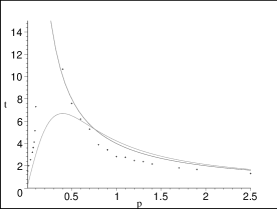
5mm normal

Figure 1: The traveltime dependence on relative momentum values.
Left – case of parallel mutual spin orientation, right – anti-parallel one.
Curve 1 corresponds to electrons travelflying over through each other; time is inversely proportional to the momentum; Curve 2 corresponds to classical Coulomb collision. Curve 3 corresponds to two coherent electrons interaction.

5mm normal

Figure 2: The dependence of quadrupole moment on time: left – typical case, right – special one.

5mm normal

Figure 3: Change of wave function of coherent electron pair is represented for a case of recession of centers of wave packages quicker than their spreading.

5mm normal

Figure 4: Change of wave function of coherent electron pair is represented, recession of centers of wave packages vanishes, instead spreading of wave packages takes place.

References

- (1) Gerardo Adesso and Fabrizio Illuminati, Bipartite And Multipartite Entanglement Of Gaussian States:- arxiv:quant-ph/0510052
- (2) Y. Nakamura, Yu.A. Pashkin, T. Yamamoto, and J.S. Tsai, Phys. Rev. Lett. 88, 047901 (2002).
- (3) John R. Klauder, Phase Space Geometry in Classical and Quantum Mechanics - Second InternationalWorkshop on Contemporary Problems in Mathematical Physics, Cotonou, Benin, October 28-November 2, 2001: arxiv:quant-ph/0112010
- (4) E. Paladino, L. Faoro, G. Falci, and R. Fazio, Phys. Rev. Lett. 88, 228304 (2002).
- (5) D. Vion, A. Aassime, A. Cottet, P. Joyez, H. Pothier, C. Urbina, D. Esteve, and M.H. Devoret, Science 296, 886 (2002).
- (6) V. O. Gnatovskyy and C.V. Usenko, Electron-electron Coulomb interaction for coherent entangled states - Fortschr. Phys. 51, No. 2-3, 134 - 138 (2003)
- (7) S.A. Gurvitz, Two-electron correlated motion due to Coulomb repulsion:- arxiv:cond-mat/0203545
- (8) C. W. J. Beenakker, C. Emary, M. Kindermann, and J. L. van Velsen, Production and detection of entangled electron-hole pairs in a degenerate electron gas arxiv:cond-mat/0305110
- (9) Lixin He, Gabriel Bester, and Alex Zunger, Singlet-triplet splitting, correlation and entanglement of two electrons in quantum dot molecules:- arxiv:cond-mat/0503492
- (10) A.V. Lebedev a, G.B. Lesovik a, and G. Blatter, Generating spin-entangled electron pairs in normal conductors using voltage pulses arxiv:cond-mat/0504583
5mm
\onelinecaptionsfalse
\captionstylenormal