Entangled mixed-state generation by twin-photon scattering

Abstract

We report experimental results on mixed-state generation by multiple scattering of polarization-entangled photon pairs created from parametric down-conversion. By using a large variety of scattering optical systems we have experimentally obtained entangled mixed states that lie upon and below the Werner curve in the linear entropy-tangle plane. We have also introduced a simple phenomenological model built on the analogy between classical polarization optics and quantum maps. Theoretical predictions from such model are in full agreement with our experimental findings.

I Introduction

The study of spatial, temporal and polarization correlations of light scattered by inhomogeneous and turbid media has a history of more than a century rayleigh . Due to the high complexity of scattering media only single-scattering properties are known at a microscopic level hulst . Conversely, for multiple-scattering processes the emphasis is mainly on macroscopic theoretical descriptions of the correlation phenomena rossum . In most examples of the latter albada1 ; chabanov ; rikken ; freund the intensity correlations of the interference pattern generated by multiple-scattered light are explained in terms of classical wave-coherence. On the other hand, the recent availability of reliable single-photon sources has triggered the interest in quantum correlations of multiple-scattered light lohdal . Generally speaking, quantum correlations of scattered photons depend on the quantum state of the light illuminating the sample. In Ref. lohdal , spatial quantum correlations of scattered light were analyzed for Fock, coherent and thermal input states.

In this paper we present the first experimental results on quantum polarization correlations of scattered photon pairs. Specifically, we study the entanglement content in relation to the polarization purity of multiple-scattered twin-photons, initially generated in a polarization-entangled state by spontaneous parametric down-conversion (SPDC). The initial entanglement of the input photon pairs will in general be degraded by multiple scattering. This can be understood by noting that the scattering process distributes the initial correlations of the twin-photons over the many spatial modes excited along the propagation in the medium. In the case of spatially inhomogeneous media the polarization degrees of freedom are coupled to the spatial degrees of freedom generating polarization dependent speckle patterns. If the spatial correlations of such patterns are averaged out by multi-mode detection, the polarization state of the scattered photon(s) is reduced to a mixture, and the resulting polarization-entanglement of the photon pairs is degraded with respect to the initial one. A related theoretical background was elaborated in aiello1 ; vanvelsen .

This paper is structured as follows: In section II we report our experiments on light scattering with entangled photons. First, we present our experimental set-up and briefly describe the many different optical systems that we used as scatterers. Next, we show our experimental results. The notions of generalized Werner and sub-Werner states are introduced to illustrate these results. In section III we introduce a simple phenomenological model for photon scattering that fully reproduces our experimental findings. Finally, in section IV we draw our conclusions.

II Experiments on light scattering with entangled photons

II.1 Experimental set-up

Our experimental set-up is shown in Fig. 1. A Krypton-ion laser at 413.1 nm pumps a 1 mm thick $\beta-\mathrm{Ba}\mathrm{B}_{2}\mathrm{O}_{4}$ (BBO) crystal, where polarization-entangled photon pairs at wavelength 826.2 nm are created by SPDC in degenerate type II phase-matching configuration sergienko . Single-mode fibers (SMF) are used as spatial filters to assure that each photon of the initial SPDC pair travels in a single transverse mode. Spurious birefringence along the fibers is compensated by suitably oriented polarization controllers (PC). The total retardation introduced by the fibers and walk-off effects at the BBO crystal are compensated by compensating crystals (CC: 0.5 mm thick BBO crystals) and half-wave plates ($\lambda/2$), in both signal and idler paths. In this way the initial two-photon state is prepared in the polarization singlet state $|\psi_{s}\rangle=(|HV\rangle-|VH\rangle)/\sqrt{2}$, where $H$ and $V$ are labels for horizontal and vertical polarizations of the two photons, respectively.

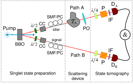
Figure 1: (Color online) Experimental scheme: After singlet preparation, the idler photon propagates through the scattering system $\mathcal{T}_{A}$. The polarization state of the scattered photon-pairs is then reconstructed via a quantum tomographic procedure (see text for details).

The experimentally prepared initial singlet state $\rho_{s}^{\mathrm{exp}}$ has a fidelity fidelity with the theoretical singlet state $\rho_{s}=|\psi_{s}\rangle\langle\psi_{s}|$ of $F(\rho_{s},\rho_{s}^{\mathrm{exp}})\sim 98\%$. In the second part of the experimental set-up the idler photon passes though the scattering device $\mathcal{T}_{A}$ before being collimated by a photographic objective (PO) with focal distance $f=5~{}\mathrm{cm}$. The third and last part of the experimental set-up, consists of two tomographic analyzers (one per photon), each made of a quarter-wave plate ($\lambda/4$) followed by a linear polarizer (P). Such analyzers permit a full tomographic reconstruction, via a maximum-likelihood technique james , of the two-photon state. Additionally, interference filters (IF) put in front of each detector ($\Delta\lambda=5$  nm) provide for bandwidth selection. Detectors $\mathrm{\textsf{D}}_{\mathrm{\textsf{A}}}$ and $\mathrm{\textsf{D}}_{\mathrm{\textsf{B}}}$ are “bucket” detectors, that is they do not distinguish which spatial mode a photon comes from, thus each photon is detected in a mode-insensitive way.

II.2 Scattering devices

All the scattering optical systems that we used were located in the path of only one of the photons of the entangled-pair (the idler one), as shown in Fig. 1. For this reason, we refer to such systems as local scatterers. Such scatterers can be grouped in three general categories according to the optical properties of the media they are made of puentes :

Type I

Purely depolarizing media, or diffusers. Such media do not affect directly the polarization state of the impinging light but change the spatial distribution of the impinging electromagnetic field.

Type II

Birefringent media, or retarders. These media introduce a polarization-dependent delay between different components of the electromagnetic field.

Type III

Dichroic media, or diattenuators. Such media introduce polarization-dependent losses for the different components of the electromagnetic field.

Type I scattering systems produce an isotropic spread in the momentum of the impinging photons. Examples of such scattering devices are: spherical-particle suspensions (such as milk or polymer micro-spheres), polymer and glass multi-mode fibers and surface diffusers. Type II scattering systems are made of birefringent media, which introduce an optical axis that breaks polarization-isotropy. Birefringence can be classified as “material birefringence” when it is an intrinsic property of the bulk medium (for example a birefringent wave-plate), and as “topological birefringence” when it is induced by a special geometry of the system that generates polarization-anisotropy, an example of a system with topological birefringence is an array of cylindrical particles. Finally, type III scattering systems are made of dichroic media that produce polarization-dependent photon absorbtion. Examples of such devices are commonly used polarizers. A systematic characterization of all the scattering devices that we used was given in Ref. puentes .

II.3 Experimental results
in the tangle versus linear entropy plane

The degree of entanglement and the degree of mixedness of the scattered photon pairs can be quantified by the tangle ($T$), namely, the concurrence squared wooters , and the linear entropy ($S_{L}$) vedral . These quantities were calculated from the $4\times 4$ polarization two-photon density matrix $\rho$, by using $T(\rho)$=(max$\{0,\sqrt{\lambda_{1}}-\sqrt{\lambda_{2}}-\sqrt{\lambda_{3}}-\sqrt{\lambda_{4}}\})^{2}$, where $\lambda_{1}\geq\lambda_{2}\geq\lambda_{3}\geq\lambda_{4}\geq 0$ are the eigenvalues of $\rho(\sigma_{2}\otimes\sigma_{2})\rho^{*}(\sigma_{2}\otimes\sigma_{2})$, where $\sigma_{2}=\left[\begin{array}[]{cc}0&-i\\ i&0\end{array}\right]$, and $S_{L}(\rho)=\frac{4}{3}[1-\mathrm{Tr}(\rho^{2})]$.

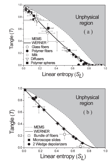
Figure 2: Experimental data in the linear entropy-tangle ($S_{L}$-$T$) plane. The grey area corresponds to unphysical density matrices. Dashed upper curve: Maximally entangled mixed states (MEMS), continuous lower curve: Werner states. (a) Polarization-isotropic scatterers (type I). (b) Birefringent scatterers (type II).

Figures 2 (a) and (b) show experimental data reported on the linear entropy-tangle plane. The position of each experimental point in such plane has been calculated from a tomographically reconstructed james two-photon density matrix $\rho^{\mathrm{exp}}$. The uniform grey area corresponds to non-physical states mems . The dashed curve that bounds the physically admissible region from above is generated by the so-called maximally entangled mixed states (MEMS) mems2 ; mems3 . The lower continuous curve is produced by the Werner states werner of the form: $\rho_{W}=p\rho_{s}+\frac{1-p}{4}I_{4}$, ($0\leq p\leq 1$), where $I_{4}$ is the $4\times 4$ identity matrix. Figure 2 (a) shows experimental data generated by isotropic scatterers (type I). Specifically, our type I scatterers consisted of the following categories. (i) Suspensions of milk and micro-spheres in distilled water, where the sample dilution was varied to obtain different points; (ii) Multi-mode glass and polymer fibers, where the tuning parameter exploited to obtain different points was the length of the fiber (cut-back method); (iii) Surface diffusers, where the full width scattering angle was used as tuning parameter. It should be noted that suspensions of milk and micro-spheres are dynamic media, where Brownian motion of the micro-particles induces temporal fluctuations within the detection integration time puentes .

In Fig. 2 (a), the experimental point at the top-left corner (nearby $T=1$, $S_{L}=0$), is generated by the un-scattered initial singlet state. The net effect of scattering systems with increasing thickness is to shift the initial datum toward the bottom-right corner ($T=0$, $S_{L}=1$), that corresponds to a fully mixed state.

Figure 2 (b) displays experimental data generated by birefringent scattering systems (type II). As an example of a system with “material birefringence” we used a pair of wedge depolarizers in cascade kliger . Different experimental points where obtained by varying the relative angle between the optical axis of the two wedges puentes2 . The systems with “topological birefringence” we considered consisted of two different devices: (i) The first one was a bundle of parallel optical fibers vdmark . Translational invariance along the fibers axes restricts the direction of the wave-vectors of the scattered photons in a plane orthogonal to the common axis of the fibers. (ii) The second device was a stack of parallel microscope slides (with uncontrolled air layers in between). This optical system is depolarizing because it amplifies any initial spread in the wave-vector of the impinging photon. This photon enters via a single-mode-fiber (numerical aperture $\mathrm{NA}=0.12$), from one side of the stack and travels in a plane parallel to the slides.

In Fig. 3, experimental data generated by dichroic scattering systems (type III) are shown. We used: (i) Surface diffusers followed by a stacks of microscope slides at the Brewster angle and (ii) Commercially available polaroid sheets with manually-added surface roughness on its front surface to provide for wave-vector spread. All data thus obtained fall below the Werner curve, generating what we called sub-Werner states, namely states with a lower value of tangle ($T$) than a Werner state, for a given value of the linear entropy ($S_{L}$).

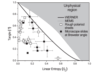
Figure 3: Experimental data generated by dichroic scattering systems (type III).

In summary, Figs. 2 (a)-(b) show that all data generated by type I and II scattering systems fall on the Werner curve, within the experimental error; while data generated by scattering samples type III, which are presented in Fig. 3, lay below the Werner curve. In Section III we shall present a simple theoretical interpretation for such results.

II.4 Error estimate

In order to estimate the errors in our measured data, we numerically generated 16 Monte Carlo sets $N_{i}$ ($i=1,\ldots,16$) of $10^{3}$ simulated photon counts, corresponding to each of the $16$ actual coincidence count measurements $\{n_{i}^{\mathrm{exp}}\}$ ($i=1,\ldots,16$) required by tomographic analysis to reconstruct a single two-photon density matrix. Each set $N_{i}$ had a Gaussian distribution centered around the mean value $\mu_{i}=n_{i}^{\mathrm{exp}}$, with standard deviation $\sigma_{i}=\sqrt{n_{i}^{\mathrm{exp}}}$. The sets $N_{i}$ where created by using the “NormalDistribution” built-in function of the program Mathematica 5.2. Once we generated the $16$ Monte Carlo sets $N_{i}$, we reconstructed the corresponding $10^{3}$ density matrices using a maximum likelihood estimation protocol, to assure that they could represent physical states. Finally, from this ensemble of matrices we calculated the average tangle $T^{\mathrm{av}}$ and linear entropy $S_{L}^{\mathrm{av}}$. The error bars were estimated as the absolute distance between the mean quantities ($\mathrm{av}$) and the measured ones ($\mathrm{exp}$): $\sigma_{T}=|T^{\mathrm{exp}}-T^{\mathrm{av}}|$, $\sigma_{S_{L}}=|S_{L}^{\mathrm{exp}}-S_{L}^{\mathrm{av}}|$. It should be noted that this procedure produces an overestimation of the experimental errors. In the cases where part of the overestimated error bars fell into the unphysical region, the length of such bars was limited to the border of the physically allowed density matrices.

II.5 Generalized Werner states

Close inspection of the reconstructed density matrices generated by type II scattering systems revealed that in some cases the measured states represented a generalized form of Werner states. These are equivalent to the original Werner states $\rho_{W}$ with respect to their values of $T$ and $S_{L}$, but the form of their density matrices is different. Werner states $\rho_{W}$ of two qubits were originally defined werner as such states which are $U\otimes U$ invariant: $\rho_{W}=U\otimes U\rho_{W}U^{\dagger}\otimes U^{\dagger}$. Here $U\otimes U$ is any symmetric separable unitary transformation acting on the two qubits. The generalized Werner states $\rho_{GW}$ we experimentally generated, can be obtained from $\rho_{W}$ by applying a local unitary operation $V$ acting upon only one of the two qubits: $\rho_{GW}=V\otimes I\rho_{W}V^{\dagger}\otimes I$, where $I=\left[\begin{array}[]{cc}1&0\\ 0&1\\ \end{array}\right]$, and

$$V(\alpha,\beta,\gamma)=\left[\begin{array}[]{cc}e^{-\frac{i}{2}(\alpha+\beta)}\cos{\gamma/2}&-e^{-\frac{i}{2}(\alpha-\beta)}\sin{\gamma/2}\\ e^{\frac{i}{2}(\alpha-\beta)}\sin{\gamma/2}&e^{\frac{i}{2}(\alpha+\beta)}\cos{\gamma/2}\\ \end{array}\right],$$ (3)

where $\alpha,\beta,\gamma$ can be identified with the three Euler angles characterizing an ordinary rotation in $\mathbb{R}^{3}$ nielsen . These generalized Werner states have the same values of $T$ and $S_{L}$ as the original $\rho_{W}$ (since a local unitary transformation does not affect neither the degree of entanglement nor the degree of purity) but are no longer invariant under unitary transformations of the form $U\otimes U$. By using Eq. (3), we calculated the average maximal fidelity of the measured states $\rho^{\mathrm{exp}}_{GW}$ with the target generalized Werner states $\rho^{\mathrm{th}}_{GW}(p,\alpha,\beta,\gamma)$. We found $\bar{F}(\rho^{\mathrm{exp}}_{GW},\rho^{\mathrm{th}}_{GW})\approx 96\%$, revealing that our data are well fitted by this four-parameter class of generalized Werner states.

III The phenomenological model

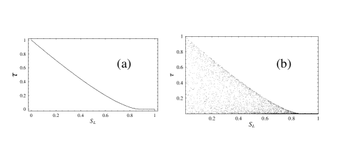
Figure 4: Numerical simulation for our phenomenological model. Fig. 4 (a) isotropic and birefringent scattering, Fig. 4 (b) dichroic scattering.

In Ref. aiello3 , a theoretical study of the analogies between classical linear optics and quantum maps was given. Within this theoretical framework it is possible to build a simple phenomenological model capable of explaining all our experimental results. To this end let us consider the experimental set-up represented in Fig. 1. The linear optical scattering element $\mathcal{T}_{A}$ inserted across path $A$ can be classically represented by some Mueller matrix $\mathcal{M}$ hulst which describes its polarization-dependent interaction with a classical beam of light. However, $\mathcal{T}_{A}$ can also be represented by a linear, completely positive, local quantum map $\mathcal{E}:\,\rho\rightarrow\mathcal{E}[\rho]$, which describes the interaction of the scattering element with a two-photon light beam encoding a pair of polarization qubits. These qubits are, in turn, represented by a $4\times 4$ density matrix $\rho$. Since $\mathcal{T}_{A}$ interacts with only one of the two photons, the map $\mathcal{E}$ is said to be local and it can be written as $\mathcal{E}=\mathcal{E}_{A}\otimes\mathcal{I}$, where $\mathcal{E}_{A}$ is the single-qubit (or single-photon) quantum map representing $\mathcal{T}_{A}$, and $\mathcal{I}$ is the single-qubit identity map.

It can be shown that the classical Mueller matrix $\mathcal{M}$ and the single-qubit quantum map $\mathcal{E}_{A}$ are univocally related. Specifically, if with $\mathcal{M}$ we denote the complex-valued Mueller matrix written in the standard basis, then the following decomposition holds:

$$\mathcal{M}=\sum_{\mu=0}^{3}\lambda_{\mu}T_{\mu}\otimes T_{\mu}^{*},$$ (4)

where $\{T_{\mu}\}$ is a set of four $2\times 2$ Jones matrices hulst , each representing a non-depolarizing linear optical element in classical polarization optics, and $\{\lambda_{\mu}\}$ are the four non-negative eigenvalues of the “dynamical” matrix $H$ associated to $\mathcal{M}$. Given Eq. (4), it is possible to show that the two-qubit quantum map $\mathcal{E}$ can be written as

$$\rho_{\mathcal{E}}=\mathcal{E}[\rho]\propto\sum_{\mu=0}^{3}\lambda_{\mu}\,T_{\mu}\otimes I\,\rho\,T_{\mu}^{\dagger}\otimes I,$$ (5)

where the proportionality symbol “$\propto$” on the right hand side of Eq. (5) accounts for a possible renormalization to ensure $\mathrm{Tr}(\rho_{\mathcal{E}})=1$. Such renormalization becomes necessary when $\mathcal{T}_{A}$ presents polarization-dependent losses (i.e., dichroism). We anticipate that when such re-normalization is necessary the map is considered non-trace preserving. We shall briefly discuss this issue in the conclusion.

With these ingredients, a phenomenological polarization-scattering model can be built as follows. First we use the polar decomposition Lu and Chipman (1996) to write an arbitrary Mueller matrix $\mathcal{M}=\mathcal{M}_{\Delta}\mathcal{M}_{B}\mathcal{M}_{D}$, where $\mathcal{M}_{\Delta}$, $\mathcal{M}_{B}$ and $\mathcal{M}_{D}$ represent a purely depolarizing element, a birefringent (or retarder) element, and a dichroic (or diattenuator) element, respectively. Specific analytical expressions for $\mathcal{M}_{\Delta}$, $\mathcal{M}_{B}$ and $\mathcal{M}_{D}$ can be found in the literature kliger . Second, we use Eq. (4) to find the quantum maps corresponding to $\mathcal{M}_{\Delta}$, $\mathcal{M}_{B}$ and $\mathcal{M}_{D}$ and, by using such maps, we calculate the scattered two-photon state $\rho_{\mathcal{E}}$. In our experimental realizations we used isotropic scatterers $\mathcal{M}_{IS}=\mathcal{M}_{\Delta}$ with isotropic depolarization factor $0\leq\Delta<1$, birefringent scattering media $\mathcal{M}_{BS}$, described in terms of the product of a purely birefringent medium $\mathcal{M}_{B}$ and an isotropic depolarizer $\mathcal{M}_{\Delta}$, i.e. $\mathcal{M}_{BS}=\mathcal{M}_{B}\mathcal{M}_{\Delta}$, and finally, dichroic scattering media $\mathcal{M}_{DS}=\mathcal{M}_{D}\mathcal{M}_{\Delta}$, which are in turn described by a product of a purely dichroic medium $\mathcal{M}_{D}$ and a purely depolarizing medium $\mathcal{M}_{\Delta}$. It should be noted that these product decompositions are not unique. Other decompositions with different orders are possible but the elements of each matrix might change, since the matrices $\mathcal{M}_{\Delta}$, $\mathcal{M}_{B}$ and $\mathcal{M}_{D}$ do not commute.

Filling in the above expressions with random numbers selected from suitably chosen ranges, we simulated all scattering processes occurring in our experiments. Fig. 4 shows a numerical simulation of the scattered states in the tangle vs. linear entropy plane, obtained with the singlet two-photon state as input state. Fig. 4 (a) corresponds to isotropic and birefringent scatterers, and Fig. 4 (b) to dichroic scatterers. The qualitative agreement between this model and the experimental results shown in Fig. 2 and Fig. 3 is manifest.

IV Conclusions

In summary, we have presented experimental results on entanglement properties of scattered photon-pairs for three varieties of optical scattering systems. In this way we were able to generate two distinct types of two-photon mixed states; namely Werner-like and sub-Werner-like states. Moreover, we have introduced a simple phenomenological model based onto the analogy between classical polarization optics and quantum mechanics of qubits, that fully reproduces our experimental findings. In the case of sub-Werner states, the phenomenological model represents a non-trace preserving quantum map. Such description might be considered controversial since a non-trace preserving local map can in principle lead to violation of causality when it describes the evolution of a composite system made of two spatially separate subsystems Aie (b). However, we argue that our measured states do not violate the signaling condition as they are post-selected by the coincidence measurement, a procedure which involves classical communication between the two detectors. Finally, we expect it to be possible to create states above the Werner curve (in particular MEMS) mems2 ; mems3 , by post-selective detection when acting on a single photon Aie (b). Work along this line is in progress in our group.

- (1) Lord Rayleigh, Philos. Mag. 47, 375 (1899); Proc. Roy. Soc. London, Ser. A 79, 399 (1907).
- (2) H. C. van de Hulst, Light Scattering by Small Particles (Dover, New York, 1981).
- (3) M. C. W. van Rossum and T. M. Nieuwenhuizen, Rev. Mod. Phys. 71, 313 (1999).
- (4) M. P. Van Albada, and A. Lagendijk, Phys. Rev. Lett. 55, 2692 (1985).
- (5) A. A Chabanov, M. Stoytchev, and A. Z. Genack, Nature (London) 404, 850 (2000).
- (6) G. L. J. A. Rikken and B. A. van Tiggelen, Nature (London) 381, 54 (1996).
- (7) F. Scheffold and G. Maret, Phys. Rev. Lett. 81, 5800 (1998).
- (8) P. Lodahl, A. P. Mosk, and A. Lagendijk, Phys. Rev. Lett 95, 173901 (2005).
- (9) A. Aiello and J. P. Woerdman, Phys. Rev. A 70, 023808 (2004).
- (10) J. L. van Velsen and C. W. J. Beenakker, Phys. Rev. A 70, 032325 (2004).
- (11) P. G. Kwiat, K. Mattle, H. Weinfurter, A. Zeilinger, A. V. Sergienko, and Y. Shih, Phys. Rev. Lett. 75, 4337 (1995).
- (12) R. Jozsa, J. Mod. Opt. 41, 2315 (1994). The fidelity between the target state and the measured state was calculated as .
- (13) D. F. V. James, P. G. Kwiat, W. J. Munro, and A. G. White, Phys. Rev. A 64, 052312 (2001).
- (14) G. Puentes, D. Voigt, A. Aiello, and J. P. Woerdman, Opt. Lett. 30, 3216 (2005).
- (15) W. K. Wootters, Phys. Rev. Lett. 80, 2245 (1998).
- (16) S. Bose, and V. Vedral, Phys. Rev. A 61, 040101(R) (2000).
- (17) W. J. Munro, D. F. V. James, A. G. White, and P. G. Kwiat, Phys. Rev. A 64, 030302(R) (2001).
- (18) N. A. Peters, J. B. Altepeter, D. A. Branning, E. R. Jeffrey, T.-C. Wei, and P. G. Kwiat, Phys. Rev. Lett. 92, 133601 (2004).
- (19) M. Barbieri, F. De Martini, G. Di Nepi, and P. Mataloni, Phys. Rev. Lett. 92, 177901 (2004).
- (20) R. F. Werner, Phys. Rev. A 40, 4277 (1989).
- (21) D. S. Kliger, J. W. Lewis, and C. E. Randall, Polarized Light in Optics and Spectroscopy (Academic Press, Inc., 1990).
- (22) G. Puentes, D. Voigt, A. Aiello, and J. P. Woerdman, Opt. Lett. 31, 2057 (2006).
- (23) M. B. van der Mark, PhD thesis, Univ. Amsterdam (1990).
- (24) M. A. Nielsen and I. L. Chuang, Quantum Computation and Quantum Information (Cambridge U. Press, 2000), Chap. 12.
- (25) J. J. Sakurai, Modern Quantum Mechanics (Addison Wesley, 1994).
- Lu and Chipman (1996) S.-Y. Lu and R. A. Chipman, J. Opt. Soc. Am. A 13, 1106 (1996).
- (27) A. Aiello, G. Puentes, and J. P. Woerdman, quant-ph/0611179, submitted to Phys. Rev. A (2006).
- Aie (b) A. Aiello, G. Puentes, D. Voigt, and J. P. Woerdman, quanth-ph/0603182 (2006).