An efficient method for scattering problems in open billiards: Theory and applications.

Abstract

We present an efficient method to solve scattering problems in two-dimensional open billiards with two leads and a complicated scattering region. The basic idea is to transform the scattering region to a rectangle, which will lead to complicated dynamics in the interior, but simple boundary conditions. The method can be specialized to closed billiards, and it allows the treatment of interacting particles in the billiard. We apply this method to quantum echoes measured recently in a microwave cavity, and indicate, how it can be used for interacting particles.

I Introduction

The role of two-dimensional billiards in the development of chaos theory in general and of wave chaos in particular is basic. The pioneering work of Sinai sinai has opened the door for a large field of research where work of Bunimovich and others bunimovich ; bunimovich1 has provided us with a number of interesting shapes, for which chaoticity (at least ergodicity and the Kolmogorov property) have been proven. This has become particularly relevant as for soft potentials, at this point, no such example was found. There is even a wide-spread belief, that no example may exist. The field got additional impulse, from the fact that in scattering systems hyperbolicity may be easily proven e.g. for the two and three disk problem Eckhardt , and for the latter there exists a bounded manifold, that is chaotic. For scattering systems this property is also achievable for soft potentials jung . The study of billiards has also proven interesting in mixed systems, both of the bound (e.g. bmushroom1 ; bmushroom2 ) and open type mejia ; friedrich .

In physics, billiards have acquired increasing importance as they are seen to represent relevant aspects of systems as small as quantum dots qdots and as large as planetary rings benet . Wave realizations of such objects have become even more popular, as experiments with flat microwave cavities become available from an ever larger number of labs stockmann1 ; stockmann2 ; richter1 ; richter2 ; richter3 ; smilansky ; sirko ; anlage ; Shridar ; legrand . Such experiments emulate single particle properties of mesoscopic devices. Furthermore such billiards provide a very direct and experimentally accessible way to test hypothesis on classical-quantum connections, such as the relation between the classical ensembles of random matrices cartan and chaotic evolution, for spectra casati ; bohigas ; berry ; leyvraz ; braun , wave-functions porter ; gorin and scattering properties seligman ; vwz .

Microwave billiards emulate the wave behavior of the corresponding classical billiard and thus they form the most direct way to test hypotheses proposed for classical-quantum or ray-wave connections. For closed billiards extremely efficient algorithms are exist vergini ; prosen , while for scattering situations only some standard finite element programs are available to solve general problems. Recently a new technique has been proposed for special situations, such as the ripple channel Akguc1 ; Akguc2 . The purpose of the present paper is to generalize this technique such that it can bee applied to typical open billiards in use as quantum dots or in microwave experiments. The basic idea is to transform the complicated border to a simple rectangle with openings. The price we pay is that we now have to deal with a much more complicated Hamiltonian instead of the simple Laplace-Beltrami operator.

The advantage of this procedure thus clearly results from the simple boundary conditions. While these also play a role for bound systems they are more pronounced in scattering systems. If we use R-matrix theory we have to implement Dirichlet and Neumann conditions in different parts of the surface simultaneously, and this becomes rather easy with the simple boundary conditions. The more complicated dynamics can be handled by in such a way, that the main numerical effort is reduced to fast Fourier transforms, which are known to be extremely efficient.

We apply our method to obtain transmission and the power spectrum for a scattering configuration with mixed hilbertspace in the interior of the cavity very similar to the one for which scattering experiments have been performed successfully in Darmstadt with a superconducting microwave cavity friedrich . We shall refer to this configuration as Darmstadt experiment configuration (or billiard) and we will show that we can reproduce the main feature, namely the scattering echo mejia , which was theoretically predicted. Also we find, that this kind of dynamics introduces a step-structure in total transmission, which should be observable in microwave billiards, though total cross-section measurements over many channels are always difficult. Furthermore we show, that two-body interactions can be introduced efficiently, thus opening the door for a plethora of additional important applications.

We shall proceed in the next section to recall some elements of S- and R-matrix theory. Furthermore we shall connect these to concepts such as reflection and transmission, much more common in the language of mesoscopics. In the section III we attack the main problem, namely to show how we transform a complicated shape to a rectangle and what operator will appear in calculation of the the R-matrix. We then obtain a general result with a well defined numerical recipe, which is mainly based on fast Fourier transforms (FFT). In section four we apply this technique to the Darmstadt experiment billiard used in friedrich to experimentally confirm the existence of scattering echoes due to large integrable islands in the classical system. Note that the original theoretical prediction for a quantum system was made generically using a simple delta-kicked one-dimensional system, and the authors there claim, that a computation of the scattering billiard is not feasible to sufficiently short wave length with available meansmejia . In the following section we open the door to further applications as we discuss, how the method can be applied for systems with two-body interactions. We then give some brief conclusions.

II Scattering in open billiards

The system we are concerned with is sketched in Fig. 1 It consist of a flat wave guide of width $w$ that supports $N$ open modes (or channels) with a rather general scattering region of length $L$. The specific method we develop, requires two leads (openings are in principle also possible) at opposing ends of a scattering region. We shall arbitrarily fix them to be on the right and on the left, as in the figure. The scattering region between n the leads or openings shall be described by two single-valued functions of a coordinate say $x$ defined between the two leads. No additional scatterers in the so defined cavity are allowed. We will assume, that the leads have equal width. The latter is not essential for the method but simplifies notation. The scattering problem will be defined in terms of a $2N\times 2N$ scattering matrix $S$. Having nano structures in mind we can rewrite the S-matrix as

$$S=\left(\begin{array}[]{cc}r&t^{\prime}\\ t&r^{\prime}\end{array}\right),$$ (1)

where $r$ ($r^{\prime}$) and $t$ ($t^{\prime}$) are the reflection and transmission matrices for incidence on the left (right) of the scattering region. The dimensionless conductance is obtained from $S$ as

$$T=\rm{tr}(tt^{\dagger}).$$ (2)

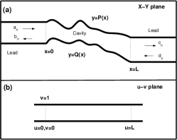
Figure 1: (a) An open billiard of length L . (b) the scattering cavity is transformed to a rectangular region in u-v plane

Our calculations will be based on the traditional R-matrix approach Wigner ; Lane . This formalism has been adapted to obtain the S matrix for a wave guide in previous works Akguc1 ; Akguc2 ; Reichl . Until now only a restricted choices of scattering regions has been investigated. For example only one of the wall was taken of sinusoidal shape while the other one was kept flat (ripple billiard). We want to generalize this approach to a generic open two-lead cavity without obstacles, where one can choose any unique differentiable function of $P(x)$ and $Q(x)$ in Fig. 1 to represent the upper and lower walls of the scattering cavity.

We wish to remind the reader, that the $R$-matrix approach relates the S-matrix to a matrix $R$ determined by boundary conditions relating internal and external functions at the edges, where the leads are connected to the scattering region, such that

$$\psi|_{\Gamma}=R\nabla\psi|_{\Gamma}$$ (3)

at $x=\Gamma$ as in of the boundaries represented as dotted lines in Fig. 1. $R$-matrix can be generalized for number of lead connection and number of modes in the leads. $R$-matrix can be related to $S$-matrix,

$$S=\frac{1-ikR}{1+ikR}$$ (4)

Rather than recalling details of $R$-matrix theory we will evoke the spirit of the method by presenting a trivial one dimensional example:

In Fig. 2 we show the 1D example we want to solve using $R$-matrix method. In this example we have 2 asymptotes as in the general case we discuss but the $r$ and $t$ are functions instead of a matrices as in the 1 mode case for the real cavity problems. The exact $S$-matrix can be found in this case and the transmission probability is given by

$$T_{exact}(E)=\frac{1}{(1+(\frac{V_{0}^{2}}{(E(E-V_{0}))(2\sin(k))^{2}})}$$ (5)

for a constant potential step of height $V_{0}$ and length 1.

Numerically we use a basis for the Reaction region,(R in Fig. 2), which is given by $cos(m\pi x),m=0,1,\dots\infty$. $x_{l}=0$ and $x_{r}=1$ have been chosen. Using this basis, the R-matrix elements are given by,

$$R_{rr}=\frac{1}{E-V_{0}}+\sum_{m=1}^{\infty}\frac{2}{E-m^{2}\pi^{2}-V_{0}}=R_{ll}$$

$$R_{rl}=\frac{1}{E-V_{0}}+\sum_{m=1}^{\infty}\frac{2\cos(m\pi)}{E-m^{2}\pi^{2}-V_{0}}=R_{lr}.$$

This series should be truncated at some finite value for a numerical calculation; $m=1000$ is used in Fig. 2. The S matrix is obtained from R matrix as

$$S=\left(\begin{array}[]{cc}1&0\\ 0&e^{-ik}\end{array}\right)\frac{\left(\begin{array}[]{cc}1&0\\ 0&1\end{array}\right)-ik\left(\begin{array}[]{cc}R_{rr}&R_{rl}\\ R_{lr}&R_{ll}\end{array}\right)}{\left(\begin{array}[]{cc}1&0\\ 0&1\end{array}\right)+ik\left(\begin{array}[]{cc}R_{rr}&R_{rl}\\ R_{lr}&R_{ll}\end{array}\right)}\left(\begin{array}[]{cc}1&0\\ 0&e^{-ik}\end{array}\right)$$

Using this S matrix we plot the transmission probability ,$|S_{1,2}|^{2}$ in Fig. 1. We note that generalizing the potential in this example to any shape can be done by using a finite difference method.Akguc3

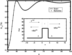
Figure 2: Scattering from a 1D barrier. The solid line shows the transmission probability as a function of energy and stars are the numerical calculations. In the inset the geometry of the scattering system is shown. $I$ indicates the interaction region, $A$ the asymptotic regions.

The method to obtain the S-Matrix thus proceeds in two steps: First obtain the solution of the boundary value problem inside the scattering region with Neumann and Dirichlet boundary conditions at lead connections and cavity walls respectively. Second connect the known solution in the asymptotic region(leads) to the one obtained for the scattering region by imposing continuity of the solution. In the method we present surprisingly the most time consuming step in numerics will be to obtain a complete set of function to expand the scattering wave function inside the cavity region, which is a prerequisite to the first step.

III The Method

We shall thus start by presenting a very efficient method to deal with the problem inside the scattering region. This method can also be applied to closed cavities, as we will point out further down. As we will use transformed coordinates the second step will not be entirely trivial and will be presented once we have the internal solutions.

III.1 Cavity Region

We want to solve the Schrödinger equation in the cavity with specific boundary conditions, namely Neumann conditions at the open boundaries, and Dirichlet conditions at the walls of the billiard. With other words, the derivative of the wave function is set to be zero at the dotted line in Fig. 1 and the wave function itself is set to zero at surface of the billiard. Thus we have the equation

$$H|\Psi(x,y)>=-\frac{\hbar^{2}}{2m}(\nabla_{x}^{2}+\nabla_{y}^{2})\Psi(x,y)=E_{n}\Psi(x,y),$$ (7)

with the boundary conditions $\nabla_{x}\Psi(x,y)|_{x=0}=0$, $\nabla_{x}\Psi(x,y)|_{x=L}=0$, $\Psi(x,y)|_{y=P(x)}=0$ and $\Psi(x,y)|_{y=Q(x)}=0$. The eigenvalues and eigenvectors of this equation are used to represent the scattering dynamics inside the cavity.

The solution of the Schrödinger equation in the coordinates $x,y$ is complicated due to the arbitrary shape of the boundaries so we use following transformation to new coordinates $u,v$.

$$u = x$$

$$v = \frac{y-Q(x)}{P(x)-Q(x)}$$ (8)

This change of variable transforms the complicated boundary to a simple one,i.e. a rectangular region. The price we pay, is that the form of the Schroedinger equation becomes more complicated. The Hamiltonian operator in the $u-v$ plane can be obtained by using the above transformation and complete derivatives. The final result is

$$H=\nabla_{u}^{2}+\left(\frac{1+(Q_{u}+vJ_{u})^{2}}{J^{2}}\right)\nabla_{v}^{2}-2\left(\frac{Q_{u}+vJ_{u}}{J}\right)\nabla_{u,v}$$

$$-\left(\frac{Q_{u,u}+vJ_{u,u}}{J}\right)\nabla_{v}+2\left(\frac{(Q_{u}+vJ_{u})J_{u}}{J^{2}}\right)\nabla_{v}$$ (9)

where $J$ is defined as $J=P-Q$ and subscripts indicate partial derivatives. In this form the symmetric nature of Hamiltonian is not obvious. Therefore we will represent the same equation in the following matrix form,dewit

$$H=\frac{1}{J}\left(\nabla_{\alpha}Jg^{\alpha,\beta}\nabla_{\beta}\right)\hskip 10.0pt\alpha=u,v\hskip 5.0pt\beta=u,v$$ (10)

where $g$ is a metric and equivalent to,

$$g\equiv\left(\begin{array}[]{cc}1&\frac{-(Q_{u}+vJ_{u})}{J}\\ \frac{-(Q_{u}+vJ_{u})}{J}&\frac{1+(Q_{u}+vJ_{u})^{2}}{J^{2}}\end{array}\right)$$ (11)

The meaning of $J$ becomes clear when we notice it is related to the determinant of the metric. It plays the role of Jacobian of the transformation from the x-y to the u-v plane. The wave function in the u-v plane can be expanded in terms of a basis

$$\Psi_{k}(u,v) = \sum_{n,m}B_{n,m}^{k}\psi_{n,m}$$ (12)

$$= \sum_{n,m}B_{n,m}^{k}\frac{1}{\sqrt{J}}\frac{2}{\sqrt{L}}\cos(\frac{m\pi u}{L})\sin(n\pi v)$$

which satisfies the boundary conditions at $u=0,u=L$ and $v=0,v=1$ automatically. To determine the unknown coefficients $B_{n,m}^{k}$ we will use the orthanormality condition. In the original coordinates plane waves are orthonormal; in terms of $u,v$ they must be orthonormal with a weight function given by the metric

$$<\Psi|\Psi>\equiv\int\int dudvJ\Psi_{k}(u,v)\Psi_{k^{\prime}}(u,v)=\delta_{k,k^{\prime}}$$ (13)

After multiplying the eigenvalue equation with another eigenfunction and integrating we obtain the matrix equation,

$$\sum_{l}\sum_{l^{\prime}}H_{ll^{\prime}}B_{l^{\prime}}^{k}=B_{l}^{k}$$ (14)

where we use new indices such that $(n,m)\rightarrow l$ and $(n^{\prime},m^{\prime})\rightarrow l^{\prime}$. Eigenvalues $E_{k}$ correspond to energy and eigenvectors contain the unknown coefficients $B_{l}^{k}$ of the wavefunction. Using the matrix form of $H$ we have,

$$\int\int dudvJ\psi_{l}\frac{1}{J}\nabla_{\alpha}Jg^{\alpha\beta}\nabla_{\beta}\psi_{l^{\prime}}=E_{k}\delta_{l,l^{\prime}}.$$ (15)

We can integrate by parts. The surface terms are zero due to the boundary condition we have chosen. We thus find

$$-\int\nabla_{\alpha}\psi_{l}Jg^{\alpha\beta}\nabla_{\beta}\psi_{l^{\prime}}=E_{k}\delta_{l,l^{\prime}}.$$ (16)

Since the metric is symmetric, the matrix obtained from this equation is real symmetric and positive definite which guarantees positive energy eigenvalues.

Once the eigenvalue equation is solved one can obtain scattering wave function for any energy within the range of wave length we allow. This makes the method efficient compared to direct integration of the differential equation by some mesh based method like finite element Akguc1 . The cut off on the number of basis states determines the accuracy and range of validity of the method. In practice it is necessary to decide how many modes to choose in $u$ and $v$ direction. A corresponding integrable geometry gives an idea about these numbers. Also one needs to choose only the lower part of the eigenvalue spectrum in the bound region to ensure that truncation wont bring errors due to poor solutions of the bounded problem. For example $m=90$ , $n=50$ and using the first 3000 eigenvalues of the 4500X4500 matrix is suitable for a rectangular region with length twice its width. The limit of the highest wavelength that can be attained in leads is connected to the lead size to the scattering size. If the size of scattering region is much bigger than the size of the leads than the method is limited to only couple of modes in leads due to the cut off on the number of eigenvalues that has to be done in cavity region. In the application we discuss in this paper this is not the case since size of cavity is smaller than leads.

We need an efficient method to calculate the matrix elements. Each matrix elements is a double integral over u and v. Due to the form of the metric and sinusoidal nature of the basis states we can achieve this writing the terms of Eq. 16 as follows:

$$< \Psi|H|\Psi>=\int du\nabla_{u}(\frac{C_{m}}{\sqrt{J}})J\nabla_{u}(\frac{C_{m^{\prime}}}{\sqrt{J}})\cdot\int dvS_{n}S_{n^{\prime}}$$

$$+ n^{\prime}\pi\int du\nabla_{u}(\frac{C_{m}}{\sqrt{J}})(-Q_{u})\frac{C_{m^{\prime}}}{\sqrt{J}}\cdot\int dvS_{n}C_{n^{\prime}}$$

$$+ n^{\prime}\pi\int du\nabla_{u}(\frac{C_{m}}{\sqrt{J}})(-J_{u})\frac{C_{m^{\prime}}}{\sqrt{J}}\cdot\int dvS_{n}vC_{n^{\prime}}$$

$$+ n\pi\int du\frac{C_{m}}{\sqrt{J}}(-Q_{u})\frac{C_{m^{\prime}}}{\sqrt{J}}\cdot\int dvC_{n}S_{n^{\prime}}$$

$$+ n\pi\int du\frac{C_{m}}{\sqrt{J}}(-J_{u})\frac{C_{m^{\prime}}}{\sqrt{J}}\cdot\int dvC_{n}vS_{n^{\prime}}$$

$$+ nn^{\prime}\pi^{2}\int duC_{m}C_{m^{\prime}}\frac{(1+Q_{u}^{2})}{J^{2}}\cdot\int dvC_{n}C_{n^{\prime}}$$

$$+ nn^{\prime}\pi^{2}\int duC_{m}C_{m^{\prime}}\frac{(2Q_{u}J_{u})}{J^{2}}\cdot\int dvC_{n}vC_{n^{\prime}}$$

$$+ nn^{\prime}\pi^{2}\int duC_{m}C_{m^{\prime}}\frac{(J_{u}^{2})}{J^{2}}\cdot\int dvC_{n}v^{2}C_{n^{\prime}}.$$

Here we use the abbreviations $C_{m}\rightarrow\cos(m\pi u/L)$, $S_{n}\rightarrow\sin(n\pi v)$ and $C_{n}\rightarrow\cos(n\pi v)$. The integral over $v$ can be performed analytically. All the terms except the first one are of the form of a function multiplying a $C_{m}$ term. These integrals can be done using a fast Fourier transform. The first term can be put in the same form, after some algebra:

$$K_{1}=(\frac{m^{2}\pi^{2}}{L^{2}}\delta_{m,m^{\prime}}-\int duC_{m}\nabla_{u}(C_{m}^{\prime})\nabla_{u}(\log(J)/2)$$

$$-\int duC_{m^{\prime}}\nabla_{u}(C_{m})\nabla_{u}(\log(J)/2)$$

$$+\int duC_{m}C_{m^{\prime}}(\nabla_{u}(\log(J)/2))^{2})$$

Therefore, when the functions $P$, $Q$ and $J$ are given as an array of dimension $M$, the integral is equal to

$$\int duC_{m}F(u)=\frac{L}{M}Re(FFT(F)_{m-1})$$ (17)

i.e. the $m-1$th element of the real part of the Fourier transform of the function is equal to the integral of the same function multiplied by $C_{m}$ . Note that one needs to incorporate end point correction Numrec to be more accurate; one way is to extend integration function symmetrically at the end point and halve the result. This is very efficient since each array of integrals is calculated by a single Fourier transform. A total of seven Fourier transform is enough to calculate all integrals for this problem. The overall matrix elements can be written using the result of exact integration in v direction as

$$<\Psi|H|\Psi>=\delta_{n,n^{\prime}}(\frac{(m-1)^{2}\pi^{2}}{L^{2}}-F_{1}(m,m^{\prime})$$

$$-F_{1}(m^{\prime},m)+F_{2}(m,m^{\prime}))$$

$$+D_{1}(n^{\prime},n)F_{3}(m^{\prime},m)+D_{2}(n,n^{\prime})F_{4}(m^{\prime},m)$$

$$+D_{1}(n,n^{\prime})F_{3}(m,m^{\prime})+D_{2}(n,n^{\prime})F_{4}(m,m^{\prime})$$

$$+D_{3}(n,n^{\prime})F_{5}(m,m^{\prime})+D_{4}(n,n^{\prime})F_{6}(m,m^{\prime})$$

$$+D_{5}(n,n^{\prime})F_{7}(m,m^{\prime}),$$ (18)

where $v$ integrals are obtained analytically,

$$D_{1}(n,n^{\prime})=(1-\delta_{n,n^{\prime}})n^{\prime}n\left(\frac{(-1+(-1)^{(n+n^{\prime})}}{(n^{\prime 2}-n^{2})}\right)$$

$$D_{2}(n,n^{\prime})=\frac{-\delta_{n,n^{\prime}}}{4}+(1-\delta_{n,n^{\prime}})nn^{\prime}\left(\frac{-1^{(n+n^{\prime})}}{(n^{\prime 2}-n^{2})}\right)$$

$$D_{3}(n,n^{\prime})=\delta_{n,n^{\prime}}(n^{2}\pi^{2}/2)$$

$$D_{4}(n,n^{\prime})=\delta_{n,n^{\prime}}(n^{2}\pi^{2}/4)+$$

$$(1-\delta_{n,n^{\prime}})nn^{\prime}\left(\frac{(-1+(-1)^{(nn-n)})(n^{2}+n^{\prime 2})}{(n^{\prime 2}-n^{2}))^{2}}\right)$$

$$D_{5}(n,n^{\prime})=\delta_{n,n^{\prime}}(n^{2}\pi^{2}/2)(1/6+1/(4n^{2}\pi^{2}))+$$

$$(1-\delta_{n,n^{\prime}})nn^{\prime}\left(\frac{2(-1)^{(nn-n)}(n^{2}+n^{\prime 2})}{(n^{\prime 2}-n^{2}))^{2}}\right)$$

and $u$ integrals

$$F_{1}(m,m^{\prime})=\frac{L}{M}Re(FFT_{m}(\nabla_{u}(C_{m^{\prime}})\nabla_{u}(log(J/2))))$$

$$F_{2}(m,m^{\prime})=\frac{L}{M}Re(FFT_{m}(C_{m^{\prime}}\nabla_{u}(log(J/2))))$$

$$F_{3}(m,m^{\prime})=\frac{L}{M}Re(FFT_{m}(-Q_{u}\nabla_{u}(\frac{C_{m^{\prime}}}{\sqrt{J}})))$$

$$F_{4}(m,m^{\prime})=\frac{L}{M}Re(FFT_{m}(-J_{u}\nabla_{u}(\frac{C_{m^{\prime}}}{\sqrt{J}})))$$

$$F_{5}(m,m^{\prime})=\frac{L}{M}Re(FFT_{m}(\frac{(C_{m^{\prime}}+C_{m^{\prime}}Q_{u}^{2})}{J^{2}}))$$

$$F_{6}(m,m^{\prime})=\frac{L}{M}Re(FFT_{m}(2C_{m^{\prime}}\frac{Q_{u}J_{u}}{J^{2}}))$$

$$F_{7}(m,m^{\prime})=\frac{L}{M}Re(FFT_{m}(C_{m^{\prime}}\frac{J_{u}^{2}}{J^{2}}))$$

The final step is to find eigenvalues and eigenvectors of this matrix which in turn gives yield the unknown expansion coefficients of the wave function in the u-v plane and obviously the energy eigenvalues. It is possible to obtain the wave function as functions of $x,y$ applying the inverse transform to the wave function in in terms of $u,v$. Since the expansion coefficients are already determined this transformation is straight forward.

III.2 Leads and Scattering Matrix

With the knowledge of states in the cavity region it is possible to couple known asymptotic, such as leads to the cavity. The corresponding solution on the left and on the right leads to

$$\Psi_{L}^{n}=\left(\frac{a_{n}}{\sqrt{k_{n}}}e^{ik_{n}x}-\frac{b_{n}}{\sqrt{k_{n}}}e^{-ik_{n}x}\right)\sin(\frac{n\pi y}{w})$$

$$\Psi_{R}^{n}=\left(\frac{c_{n}}{\sqrt{k_{n}}}e^{-ik_{n}x}-\frac{d_{n}}{\sqrt{k_{n}}}e^{ik_{n}x}\right)\sin(\frac{n\pi y}{w})$$

where $w$ is the lead width, $a_{n}$, $b_{n}$,$c_{n}$ and, $d_{n}$ are scattering amplitudes and the wave vector is given by

$$k_{n}=\sqrt{\left(\frac{n\pi}{w}\right)^{2}-\frac{2mE}{\hbar^{2}}}.$$ (22)

We here assume propagating modes but it is possible to add evanescent modes with complex k vectors to the calculation. Their effect is discussed in ref. Akguc2

As shown in references Akguc1 Akguc2 Reichl the energy eigenfuntions $|E>$ of the total scattering system have contributions from both cavity and leads.

$$<x,y|E>=\sum_{j=1}^{\infty}\gamma_{j}\phi_{j}(x,y)+\sum_{n=1}^{\infty}(\Gamma_{n}^{L}\Psi_{L}^{n}+\Gamma_{n}^{R}\Psi_{R}^{n})$$ (23)

where $\phi_{j}$ are basis states calculated for the cavity alone.

The continuity of scattering wave functions at the lead boundary gives the connection between the leads and the cavity region:

$$\Psi_{n}^{\alpha}=\sum_{n^{\prime}=1}^{\infty}R_{\alpha L}(n,n^{\prime})\nabla_{x}\Psi_{n}^{\alpha}|_{x_{L}}$$

$$-\sum_{n^{\prime}=1}^{\infty}R_{\alpha R}(n,n^{\prime})\nabla_{x}\Psi_{n}^{\alpha}|_{x_{R}}$$

where

$$R_{\alpha\beta}(n,n^{\prime})=\frac{\hbar^{2}}{2m}\sum_{j=1}^{\infty}\frac{\phi_{j,n}(x_{\alpha})\phi_{j,n^{\prime}}(x_{\beta})}{E-\gamma_{j}}$$ (25)

is the (n,n’)th matrix element of the R matrix. Here $\phi_{j,n}$ is the overlap between cavity states and lead functions and given by

$$\phi_{j,n}(x_{\alpha})=\sqrt{\frac{2}{L}}\int_{0}^{\infty}dy\phi_{j}(x_{\alpha})\sin(\frac{n\pi y}{w})$$ (26)

where $\alpha\equiv L,R$ and $x_{L}=0$, $X_{R}=L$ in Fig. 1.

IV Application: Quantum echoes from cavities with a large integrable island

As an application of our method we solve the scattering problem in the Darmstadt-experiment geometry shown in Fig. 3. A similar geometry to Fig. 3(a) has been used in recent experiments friedrich . The analytical curves of upper and lower wall in Fig. 3a(a) are given as follows,

$$P(x)=\lambda\exp(-\frac{\alpha x^{2}}{\lambda^{2}})\hskip 14.22636ptand\hskip 14.22636ptQ(x)=\lambda\left(\beta-\frac{\gamma x^{2}}{\lambda^{2}}\right).$$ (27)

We use the same parameters as in experiment such as $\alpha=0.161$, $\beta=0.2$ and $\gamma=0.1$. While in experiment a scaling factor of $\lambda=5cm$ is used we use $\lambda=0.432$ in arbitrary units and we shift the origin of the coordinates to the beginning of the left lead for convenience.Note though, that the original experiment does not connect to leads! Rather the opening is arbitrary, though in fact naturally finite. We will return to these differences later.

Apart from the original geometry we also consider a geometry with some small irregularity in the center of the cavity. Such an irregularity should destroy the stability of the central periodic orbit in the classical system and thus at least damage or deform the large regular island significantly. This corresponds to the mentions introduction of a perturbing scatterer in the experiment, which destroyed the echo friedrich . Furthermore we consider that the entire parabolic wall may perturbed in a disordered way.

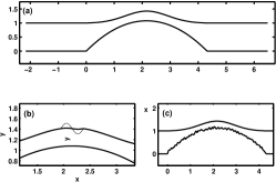
Figure 3: (a) The Darmstadt-experiment geometry of length $L=4.32$ with leads $W=1$. (b)same as in (a) but with some small disorder in the middle of the billiard. (c) The lower wall in (a) has been replaced by a disordered wall.

After calculating the S matrices for these systems we found the total conductance as described in section 1. The results for the 3 different geometries can be seen in Fig. 4. We see that for the geometry used in experiment there are steps in the conductance. These steps do not correspond to the opening of channels in the leads. This is because of the smaller width of the scattering region. The minimum width in channel is $w_{min}=0.3097$ with corresponding $k_{eff}=3.23$ matches where the first step seems to start in Fig. 4. With other words, this is the point where we pass from evanescent or tunneling transmission to open channels in the necks presented by the Darmstadt-experiment configuration.

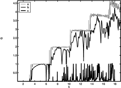
Figure 4: Conductance versus wave vector for 3 different geometries corresponding to (a), (b) and (c) in Fig. 3

While the initial rise thus is rather trivial, the step structure is not, as is sensitive to even a small disturbance. The solid line in Fig 4 shows the total conductance through the same geometry but with a small wiggle at the center of the cavity. The exact shape of the wiggle is not very relevant. We choose a sinusoidal perturbation of the upper wall in the form $0.01\sin(10\pi x_{s}/L)$ where $x_{s}$ is the x coordinate in the interval, $9L/20<x_{s}<11L/20$. (In Fig. 4 a 10 times bigger scaled version of perturbation is also shown to give an idea of the shape of perturbation.) The effect of perturbation is huge on conductance data. The step structure tends to be lost for higher energies.

We also show the result of surface disorder on conductance by the dot-dashed curve in Fig.4. We implemented surface disorder by first dividing the boundary curve into $n$ pieces and move these pieces by a random amount, $\eta$ in y direction. We apply a spline interpolation to connect the pieces to form a smooth boundary. We see that for $\eta=0.2$ and $n=100$ the step structure is lost and only resonance transmission can be seen. We note that a partial step can be observed for small disorder parameters.

We calculate the length spectrum by taking a Fourier transform of the transmission amplitude

$$t_{nm}(L)=\int_{k_{min}}^{k_{max}}dk_{F}t_{nm}(k_{F})\exp(-ik_{F}L).$$ (28)

This identification can be done based on a semi-classical description where one can sum over different periodic orbits to get the transmission amplitudes gutz . In Fig. 5 we show this quantity for $t_{11}(L)$ over an interval $1<k_{F}<19$ with $k$ in units of $\pi/w$. Note that in this interval we have a an increasing transmission matrix size each time a channel opens. we added the first element of each transmission matrix to form $t_{11}$ over the given k interval.

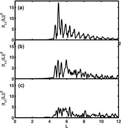
Figure 5: (a) The length spectrum for the geometry in Fig. 4(a),(b) same for the geometry in Fig. 4(b) (c) same for the geometry in Fig. 4(c).

In Fig. 5a we see the periodic oscillations starting at $L=4.32$. Since length can be associated to time for a constant speed, such as expected in an electromagnetic cavity, this is similar to the echos observed in experiment. The period seems to be constant in the data with a second harmonic entering at higher lengths suggesting a shortening in the period. In the experiment a slight shortening of the period for short times appears.This we do not see. On the other hand the experiment does not show the drastic shortening with the higher harmonics. We mus keep in mind, that the problems are not identical, because of the finite diameter leads we attached here. Also we measure transmission to the entire channel, rather than to an antenna placed near a semi-cclassically significant manifold as the latter is not meaningful in a billiard with leads. On the other hand effects of truncation must be studied carefully in each case. At this point we wish to stress, that the semi-classical structure associated with the scattering echoes again is easily seen, and – as in the experiment – for wave length far from semi-classics.

To get a better impression we look at the power spectrum for the geometry in Fig. 3(a). In Fig. 6(a) we show this spectrum calculated from $k(\pi/w)=6$ to $k(\pi/w)=9$. Since the minimum transmission matrix is 6X6 we sum over 6 modes. This region roughly corresponds to the third plateau in Fig. 4.

$$P=\sum_{n=1}^{n=6}\sum_{m=1}^{m=6}|t_{nm}(L)|^{2},$$ (29)

where $t_{nm}$ is calculated using equation 28 but with appropriate limits for k integration. In this figure we obtain peak values at $L_{1}=4.78$, $L_{2}=6.65$, $L_{3}=8.05$ ,$L_{4}=9.1$,$L_{5}=10.2$. The peak value corresponds to the simplest direct transmission orbit starting at the middle of the channel opening and hitting the center of Gaussian shaped wall before exit. As it can be seen here period decreases with increasing length. We observe oscillations up to high lengths as can be seen in inset.

We also show similar calculations in the interval $k(\pi/w)=10<k(\pi/w)<k(\pi/w)=13$ including 10 modes in Fig.6(b). Although we have different limits to the integration and different size of the matrix. We get results very similar to those the Fig. 6(a).

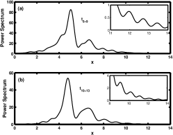
Figure 6: (a) Power spectrum from $k(\pi/d)=6$ to $k(\pi/d)=9$ including 6 modes. (b)Power spectrum from $k(\pi/d)=10$ to $k(\pi/d)=13$ including 10 modes.

V Toward many-body problems

Real naosystems have interacting particles, and treatment of such systems is incipient. We shall show, that the methods presented here is very promising for such situations, at least as long as the particles enter or leave the quantum dot only one at a time. The basic problem he consists of treating two-body interactions, as we may typically encounter in a few-body system. The two particle inside a wave guide will provide the main difficulty. It is also an important system on its own right (see the review in Leon ).

Lets consider two particles inside a cavity region as shown in Fig. 1. We will omit the problems associated with anti-symmetrization or symmetrization for Fermions or Bosons respectively, by assuming distinguishable particles, but standard methods can be used to take care of the corresponding symmetry adaption as necessary. The total Hamiltonian is,

$$H=\nabla_{x_{1}}^{2}+\nabla_{y_{1}}^{2}+\nabla_{x_{2}}^{2}+\nabla_{y_{2}}^{2}+V(|x_{1}-x_{2}|,|y_{1}-y_{2}|)$$ (30)

with a potential $V$ which depends on the distance of the two particles. The interaction term can be written in terms of single particle wave functions as follows,

$$H_{ijkl} = \int\int dx_{1}dx_{2}dy_{1}dy_{2}\phi_{i}(x_{1},y_{1})\phi_{j}(x_{2},y_{2})$$

$$V (| x_{1}-x_{2}|,|y_{1}-y_{2}|)\phi_{k}(x_{1},y_{1})\phi_{l}(x_{2},y_{2})$$ (31)

where $\phi_{i}(x,y)$ is the single particle solution in the cavity. Energies of the interacting particle can be found after diagonalizing this matrix. As the form of the single particle functions is not simple this is not an easy calculation. But as we discussed in this paper, we can transform this integration to u-v plane where we know the expansion of the single particle eigenfunctions in terms of simple harmonics. In u-v coordinates the distance between particles wont be a line but a curve given by the metric. The matrix element in u-v coordinates becomes,

$$H_{ijkl} = \int\int du1du2dv1dv2\phi^{i}(u1,v1)\phi^{j}(u2,v2)$$ (32)

$$V (u1,u2,v1,v2)\phi^{k}(u1,v1)\phi^{l}(u2,v2)$$

where $\phi^{i}(u,v)=\sum_{mn}B_{m,n}^{i}\cos(m\pi u/L)\sin(n\pi v)$ with coefficients $B_{m,n}^{i}$ calculated from a single particle equation. The harmonic expansion makes the integration simple.

VI conclusion

We present a new method to treat open billiards, that has significant advantages over older techniques. It is designed for billiards with two leads, though generalizations are possible. The basic limitation is that both irregular boundaries that connect the leads be single valued functions of some space coordinate, that connects the center of the two leads. We then transformed the scattering region into a rectangle and calculate the quantum dynamics which become involved. The boundary conditions now result trivial, and this allows to calculate the R-matrix easily and thus solve the scattering problem. It is possible to write the dynamics of two or more interacting particles in this form, as long as we do not attempts to transform to relative and center of mass coordinates. This would destroy0y the simple boundary conditions. To show the power of the method we calculated the quantum scattering echoes for such a two lead structure very near to one actually used in a microwave experiment. The results of this experiment were not accessible to a numerical calculation with standard microwave programs, but we obtained results essentially consistent with experiment, though we see a secondary effects not apparent in the experiment. Future research will have to show whether this effect is suppressed in the experiment, whether it is due to the use of leads or whether it is a consequence of the cutoff we use. This should not distract from the fact, that the main effect can be seen clearly. Concerning the example we also note that the calculation reveals a step structure in the transmission, which is directly related to the scattering echoes and was not previously noted.

Acknowledgments

The authors are grateful for useful discussions to C. Jung. Financial support under DGAPA project IN191603 and CONACyT project 43375 is acknowledged.

References

- (1) Ya. G. Sinai, Russ. Math. Surv. 25, 137 (1970).
- (2) L.A. Bunimovich, Funct. Anal. Appl. 8, 254 (1974);
- (3) L. Bunimovich, G. Casati, and I. Guarneri Phys. Rev. Lett. 77, 2941 (1996)
- (4) B. Eckhardt J. Phys. A 20, 5971 (1987)
- (5) C. Jung and H.J. Scholz, J. Phys. A 20, 3607, (1987); C. Jung and P. Richter J. Phys. A 23, 2874 (1990)
- (6) L. A. Bunimovich, Chaos 11, 802 808 (2001).
- (7) Lansel, Steven; Porter, Mason A.; and Bunimovich, Leonid A. Chaos, Vol. 16, No. 1 013129. (2006)
- (8) C. Dembowski, B. Dietz, T. Friedrich, H.-D. Graf, A. Heine, C. Mejia-Monasterio, M. Miski-Oglu, A. Richter, and T. H. Seligman Phys. Rev. Lett. 93(13) 134102, (2004)
- (9) C. Jung, C. Mejia and T.H. Seligman, Europhys. Lett. 55 616 (2001) C. Jung et al., New J. Phys. 6, 48 (2004)
- (10) C. M. Marcus, A. J. Rimberg, R. M. Westervelt, P. F. Hopkins, and A. C. Gossard, Phys. Rev. Lett. 69, 506 (1992).
- (11) L. Benet and T.H. Seligman, Phys. Lett. A 273, 331 (2000); L. Benet, J. Broch, O. Merlo and T. H. Seligman, Phys. Rev. E. 71 036225 (2005).
- (12) H. J. Stóckmann and J. Stein, Phys. Rev. Lett. 64, 2215 (1990). J. Stein and H. J. Stóckmann, Phys. Rev. Lett. 68, 2867 (1992).
- (13) Y.-H. Kim, M. Barth, H. J. Stóckmann, J. P. Bird, Phys. Rev. B 65, 165317 2002.
- (14) H. D. Gráf, H. L. Harney, H. Lengeler, C. H. Lewenkopf, C. Rangacharyulu, A. Richter, P. Schardt, and H. A. Weidenmuller, Phys. Rev. Lett. 69, 1296 (1992).
- (15) C. Dembowski, B. Dietz, H. D. Gráf, A. Heine, T. Papenbrock, A. Richter, and C. Richter, Phys. Rev. Lett.89, 064101 (2002).
- (16) R. Hofferbert, H. Alt, C. Dembowski, H. D. Gráf, H. L. Harney, A. Heine, H. Rehfeld, and A. Richter, Phys. Rev. E 71, 046201 (2005).
- (17) E. Doron, U. Smilansky and A. Frenkel, Phys. Rev. Lett. 65, 3072 (1990)
- (18) S. Deus, P.M. Koch and L. Sirko, Phys. Rev. E 52,1146 (1995)
- (19) S. Shridar, Phys. Rev. E 67, 785 (1991)
- (20) D.H. Wu et. al. Phys. Rev. Lett. 81, 2890 (1998)
- (21) J. Barthlemy, O. legrand and M. Montessagne, Phys. Rev. E 71,016205 (2005)
- (22) E. Cartan, Abh. Math. Sem. Univ. Hamburg, 11 116 (1035)
- (23) G. Casati, F. Valz-Gris and I. Guarneri, Lett. Nuovo Cimento 28, 279 (1980)
- (24) O. Bohigas, M. J. Giannoni, and C. Schmit Phys. rev. Lett. 52, 1 (1984)
- (25) M. V. Berry, Chaotic Behaviour of Deterministic Systems, edited by G. Iooss, R. Helleman, and R. Stora (North-Holland, Amsterdam), (1983),
- (26) F. Leyvraz and T. H. Seligman, Phys. Lett.A 168, 348 (1992)
- (27) S. M ller, S. Heusler, P. Braun, F. Haake, and A. Altland Phys. Rev. Lett. 93, 014103 (2004)
- (28) C.E. Porter, R.G. Thomas, Phys. Rev. 104, 483 (1956)
- (29) T Gorin, Tomaz Prosen, T. H. Seligmann New J. Phys. 6 20, (2004)
- (30) J. Verbaarschot, H.A. Weidemueller and M. Zirnbauer, Phys. Rep. 129 3672 (1985)
- (31) C. Jung, C. Lipp, and T. H. Seligman, Ann. Phys. (N.Y.) 275, 151 (1999)
- (32) E. Vergini and M. Saraceno, Phys. Rev. E 52, 2204 (1995).
- (33) Tomaz Prosen, Phys. Rev. E, 60 1658 (1999)
- (34) E.P. Wigner and L. Eisenbud, Phys. Rev. 72, 29 (1947)
- (35) A.M. Lane and R. G. Thomas, Rev. Mod. Phys. 30, 257 (1958)
- (36) L. E. Reichl The transition to Chos, Second Edition (Springer-Verlag, 2004.)
- (37) H. Feshbach Topics in the Theory of Nuclear Reactions, in Reaction Dynamics, (Gordon and Breach, New York, 1973).
- (38) G. B. Akguc and L. E. Reichl, Phys. Rev. E 67, 46202 (2003).
- (39) G. B. Akguc and L. E. Reichl, Phys. Rev. E 64, 56221 (2001).
- (40) L. E. Reichl, G. B. Akguc Found. of Phys. 31, 243 (2001).
- (41) Bryce S. DeWitt, Rev. Mod. Phy. 29 377 (1957)
- (42) William H. Press, Saul A. Teukolsky, William T. Vetterling, Brian P. Flannery, Numerical Recipes in Fortran.:The Art of Scientific Computing Second Edition. Cambridge University Press 1992
- (43) M.C. Gutzwiller, Chaos in classical and quantum mechanics, Springer 1990.
- (44) Leonid I. Glazman and Michael Pustilnik, Nanophysics: Coherence and Transport eds. H. Bouchiat et al. (Elsevier, 2005), pp. 427-478