Abstract

This work gives a detailed investigation of matrix product state (MPS) representations for pure multipartite quantum states. We determine the freedom in representations with and without translation symmetry, derive respective canonical forms and provide efficient methods for obtaining them. Results on frustration free Hamiltonians and the generation of MPS are extended, and the use of the MPS-representation for classical simulations of quantum systems is discussed.

1 Introduction and Overview

The notorious complexity of quantum many-body systems stems to a large extent from the exponential growth of the underlying Hilbert space which allows for highly entangled quantum states. Whereas this is a blessing for quantum information theory—it facilitates exponential speed-ups in quantum simulation and quantum computing—it is often more a curse for condensed matter theory where the complexity of such systems make them hardly tractable by classical means. Fortunately, physical interactions are local such that states arising for instance as ground states from such interactions are not uniformly distributed in Hilbert space. Hence, it is desirable to have a representation of quantum many-body states whose correlations are generated in a ‘local’ manner. Despite the fact that it is hard to make this picture rigorous, there is indeed a representation which comes close to this idea—the matrix product state (MPS) representation. In fact, this representation lies at the heart of the power of the density matrix renormalization group (DMRG) method and it is the basis for a large number of recent developments in quantum information as well as in condensed matter theory.

This work gives a detailed investigation of the MPS representation with a particular focus on the freedom in the representation and on canonical forms. The core of our work is a generalization of the results on finitely correlated states in [1] to finite systems with and without translational invariance. We will mainly discuss exact MPS representations throughout and just briefly review results on approximations in Sec.6. In order to provide a more complete picture of the representation and its use we will also briefly review and extend various recent results based on MPS, their parent Hamiltonians and their generation. The following gives an overview of the article and sketches the obtained results:

• Sec.2 will introduce the basic notions, provide some examples and give an overview over the relations between MPS and the valence bond picture on the one hand and frustration free Hamiltonians and finitely correlated states on the other.

• In Sec.3 we will determine the freedom in the MPS representation, derive canonical forms and provide efficient ways for obtaining them. Cases with and without translational invariance are distinguished. In the former cases we show that there is always a translational invariant representation and derive a canonical decompositions of states into superpositions of ‘ergodic’ and periodic states (as in [1]).

• Sec.4 investigates a standard scheme which constructs for any MPS a local Hamiltonian, which has the MPS as exact ground state. We prove uniqueness of the ground state (for the generic case) without referring to the thermodynamic limit, discuss degeneracies (spontaneous symmetry breaking) based on the canonical decomposition and review results on uniform bounds to the energy gap.

• In Sec.5 we will review the connections between MPS and sequential generation of multipartite entangled states. In particular we will show that MPS of sufficiently small bond dimension are feasible to generate in a lab.

• In Sec.6 we will review the results that show how MPS efficiently approximate many important states in nature; in particular, ground states of 1D local Hamiltonians. We will also show how the MPS formalism is crucial to understand the need of a large amount of entanglement in a quantum computer in order to have a exponential speed-up with respect to a classical one.

2 Definitions and Preliminaries

2.1 MPS and the valence bond picture

We will throughout consider pure quantum states $|\psi\rangle\in\mathbb{C}^{\otimes d^{N}}$ characterizing a system of $N$ sites each of which corresponds to a $d$-dimensional Hilbert space. A very useful and intuitive way of thinking about MPS is the following valence bond construction: consider the $N$ parties (’spins’) aligned on a ring and assign two virtual spins of dimension $D$ to each of them. Assume that every pair of neighboring virtual spins which correspond to different sites are initially in an (unnormalized) maximally entangled state $|I\rangle=\sum_{\alpha=1}^{D}|\alpha,\alpha\rangle$ often referred to as entangled bond. Then apply a map

$${\cal A}=\sum_{i=1}^{d}\sum_{\alpha,\beta=1}^{D}A_{i,\alpha,\beta}|i\rangle\langle\alpha,\beta|$$ (1)

to each of the $N$ sites. Here and in the following Greek indices correspond to the virtual systems. By writing $A_{i}$ for the $D\times D$ matrix with elements $A_{i,\alpha,\beta}$ we get that the coefficients of the final state when expressed in terms of a product basis are given by a matrix product $\operatorname{tr}\left[A_{i_{1}}A_{i_{2}}\cdots A_{i_{N}}\right]$. In general the dimension of the entangled state $|I\rangle$ and the map ${\cal A}$ can both be site-dependent and we write $A_{i}^{[k]}$ for the $D_{k}\times D_{k+1}$ matrix corresponding to site $k\in\{1,\ldots,N\}$. States obtained in this way have then the form

$$|\psi\rangle=\sum_{i_{1},\ldots,i_{N}=1}^{d}\operatorname{tr}\left[A_{i_{1}}^{[1]}A_{i_{2}}^{[2]}\cdots A_{i_{N}}^{[N]}\right]|i_{1},i_{2},\ldots,i_{N}\rangle\;,$$ (2)

and are called matrix product states [2]. As shown in [7] every state can be represented in this way if only the bond dimensions $D_{k}$ are sufficiently large. Hence, Eq.(2) is a representation of states rather than the characterization of a specific class. However, typically states are referred to as MPS if they have a MPS-representation with small $D=\max_{k}D_{k}$ which (in the case of a sequence of states) does in particular not grow with $N$. Note that $\psi$ in Eq.(2) is in general not normalized and that its MPS representation is not unique. Normalization as well as other expectation values of product operators can be obtained from

$$\langle\psi|\bigotimes_{k=1}^{N}S_{k}|\psi\rangle = \operatorname{tr}\left[\prod_{k=1}^{N}E_{S_{k}}^{[k]}\right]\;,\quad\text{with}$$

$$E_{S}^{[k]} \equiv \sum_{i,j=1}^{d}\langle i|S|j\rangle\overline{A}_{i}^{[k]}\otimes A_{j}^{[k]}\;.$$ (3)

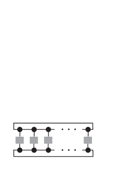
Figure 1: Computing an expectation value of an MPS is equivalent to contract the tensor of the figure, where bonds represent indices that are contracted. The matrices associated to each spin are represented by the circles (the vertical bond of each matrix is its physical index) and observables are represented by squares. It is trivial to see that this contraction can be done efficiently.

2.2 Finitely correlated states

The present work is inspired by the papers on finitely correlated states (FCS) which in turn generalize the findings of Affleck, Kennedy, Lieb and Tasaki (AKLT) [3]. In fact, many of the results we derive are extensions of the FCS formalism to finite and/or non-translational invariant systems. For this reason we will briefly review the work on FCS. A FCS is a translational invariant state on an infinite spin chain which is constructed from a completely positive and trace preserving map $\mathbb{E}:{\cal B}({\cal H}_{A})\rightarrow{\cal B}({\cal H}_{A}\otimes{\cal H}_{B})$ and a corresponding fixed point density operator $\Lambda=\operatorname{tr}_{B}[\mathbb{E}(\Lambda)]$. Here ${\cal H}_{B}=\mathbb{C}^{d}$ is the Hilbert space corresponding to one site in the chain and ${\cal H}_{A}=\mathbb{C}^{D}$ is an ancillary system. An $n$-partite reduced density matrix $\rho_{n}$ of the FCS is then obtained by repeated application of $\mathbb{E}$ to the ancillary system (initially in $\Lambda$) followed by tracing out the ancilla, i.e.,

$$\rho_{n}=\operatorname{tr}_{A}\big{[}\mathbb{E}^{n}(\Lambda)\big{]}\;.$$ (4)

An important instance are purely generated FCS where $\mathbb{E}(x)=V^{\dagger}xV$ is given by a partial isometry $V$. The latter can be easily related to the $A$’s in the matrix product representation via $V=\sum_{i=1}^{d}\sum_{\alpha,\beta=1}^{D}A_{i,\alpha,\beta}|\alpha\rangle\langle\beta i|$. Expressed in terms of the matrices $A_{i}$ the isometry condition and the fixed point relation read

$$\sum_{i=1}^{d}A_{i}A_{i}^{\dagger}=\mathbbm{1}\;,\qquad\sum_{i=1}^{d}A_{i}^{\dagger}\Lambda A_{i}=\Lambda\;,$$ (5)

which already anticipates the type of canonical forms for MPS discussed below. As shown in [4] purely generated FCS are weakly dense within the set of all translational invariant states on the infinite spin chain. Moreover, a FCS is ergodic, i.e., an extreme point within all translational invariant states, iff the map $\mathcal{E}(x)=\sum_{i}A_{i}xA_{i}^{\dagger}$ has a non-degenerate eigenvalue 1 (i.e., $\mathbbm{1}$ and $\Lambda$ are the only fixed points in Eq.(5)). Every FCS has a unique decomposition into such ergodic FCS which in turn can be decomposed into $p$ $p$-periodic states each of which corresponds to a root of unity $\exp(\frac{2\pi i}{p}m)$, $m=0,\ldots,p-1$ in the spectrum of $\mathcal{E}$. A FCS is pure iff it is purely generated and 1 is the only eigenvalue of $\mathcal{E}$ of modulus 1. In this case the state is exponentially clustering, i.e., the connected two-point correlation functions decay exponentially

$$\langle S_{i}\otimes\mathbbm{1}^{\otimes l-1}\otimes S_{i+l}\rangle-\langle S_{i}\rangle\langle S_{i+l}\rangle={\cal O}\big{(}|\nu_{2}|^{l-1}\big{)}\;,$$ (6)

where $\nu_{2}$ ($|\nu_{2}|<1$) is the second largest eigenvalue of $\mathcal{E}$.

2.3 Frustration free Hamiltonians

Consider a translational invariant Hamiltonian on a ring of $N$ $d$-dimensional quantum systems

$$H=\sum_{i=1}^{N}\tau^{i}\big{(}h\big{)}\;,$$ (7)

where $\tau$ is the translation operator with periodic boundary conditions, i.e., $\tau\big{(}\bigotimes_{i=1}^{N}x_{i}\big{)}=\bigotimes_{i=1}^{N}x_{i+1}$ where sites $N+1$ and $1$ are identified. The interaction is called $L$-local if $h$ acts non-trivially only on $L$ neighboring sites, and it is said to be frustration free with respect to its ground state $\phi_{0}$ if the latter minimizes the energy locally in the sense that $\langle\phi_{0}|H|\phi_{0}\rangle=\inf_{\phi}\langle\phi|H|\phi\rangle=N\inf_{\phi}\langle\phi|h|\phi\rangle$. As proven in [5] all gapped Hamiltonians can be approximated by frustration free ones if one allows for enlarging the interaction range $L$ up to ${\cal O}(\log N)$.

For every MPS and FCS $\psi$ one can easily find frustration free Hamiltonians such that $\psi$ is their exact ground state. Moreover, these parent Hamiltonains are $L$-local with $L\sim 2\log D/\log d$ and they allow for a detailed analysis of the ground state degeneracy (Sec.4.1) and the energy gap above the ground state (Sec.4.2). Typically, these Hamiltonians are, however, not exactly solvable, i.e., information about the excitations might be hard to obtain.

2.4 Examples

1. AKLT: The father of all matrix product states is the ground state of the AKLT-Hamiltonian

   $$H=\sum_{i}\vec{S}_{i}\vec{S}_{i+1}+\frac{1}{3}\Big{(}\vec{S}_{i}\vec{S}_{i+1}\Big{)}^{2}\;,$$ (8)

   where $\vec{S}$ is the vector of spin-1 operators (i.e., d=3). Its MPS representation is given by $\{A_{i}\}=\big{\{}\sigma^{z},\sqrt{2}\sigma^{+},-\sqrt{2}\sigma^{-}\big{\}}$ where the $\sigma$’s are the Pauli matrices.

2. Majumdar-Gosh: The Hamiltonian

   $$H=\sum_{i}2\vec{\sigma}_{i}\vec{\sigma}_{i+1}+\vec{\sigma}_{i}\vec{\sigma}_{i+2}\;$$ (9)

   is such that every ground state is a superposition of two 2-periodic states given by products of singlets on neighboring sites. The equal weight superposition of these states is translational invariant and has an MPS representation

   $$A_{1}=\left(\begin{array}[]{ccc}0&1&0\\ 0&0&-1\\ 0&0&0\\ \end{array}\right)\;,\quad A_{2}=\left(\begin{array}[]{ccc}0&0&0\\ 1&0&0\\ 0&1&0\\ \end{array}\right)\;.$$ (10)

3. GHZ states of the form $|\psi\rangle=|++\ldots+\rangle+|--\ldots-\rangle$ have an MPS representation $A_{\pm}=\mathbbm{1}\pm\sigma^{z}$. Anti-ferromagnetic GHZ states would correspond to $A_{\pm}=\sigma^{\pm}$.

4. Cluster states are unique ground states of the three-body interactions $\sum_{i}\sigma^{z}_{i}\sigma^{x}_{i+1}\sigma^{z}_{i+2}$ and represented by the matrices

   $$A_{1}=\left(\begin{array}[]{cc}0&0\\ 1&1\\ \end{array}\right)\;,\quad A_{2}=\left(\begin{array}[]{cc}1&-1\\ 0&0\\ \end{array}\right)\;.$$

5. W-states can for instance appear as ground states of the ferromagnetic XX model with strong transversal magnetic field. A W-state is an equal superposition of all translates of $|100\ldots 00\rangle$. For a simple MPS representation choose $\{A_{1}^{[k]},A_{2}^{[k]}\}$ equal to $\{\sigma^{+},\mathbbm{1}\}$ for all $k<N$ and $\{\sigma^{+}\sigma^{x},\sigma^{x}\}$ for $k=N$. Although the state itself is translational invariant there is no MPS representation with $D=2$ having this symmetry.

3 The canonical form

The general aim of this section will be to answer the following questions about the MPS representation of a given pure state:

Question 1

Which is the freedom in the representation?

Question 2

Is there any canonical representation?

Question 3

If so, how to get it?

We will distinguish two cases. The general case, or the case of open boundary conditions (OBC) and the case in which one has the additional properties of translational invariance (TI) and periodic boundary conditions (PBC).

3.1 Open boundary conditions

A MPS is said to be written with open boundary conditions (OBC) if the first and last matrices are vectors, that is, if it has the form

$$|\psi\rangle=\sum_{i_{1},\ldots,i_{N}}A^{[1]}_{i_{1}}A^{[2]}_{i_{2}}\cdots A^{[N-1]}_{i_{N-1}}A^{[N]}_{i_{N}}|i_{1}\cdots i_{N}\rangle,$$ (11)

where $A^{[m]}_{i}$ are $D_{m}\times D_{m+1}$ matrices with $D_{1}=D_{N+1}=1$. Moreover, if $D=\max_{m}D_{m}$ we say that the MPS has (bond) dimension $D$. The following is shown in [7]:

Theorem 1 (Completeness and canonical form)

Any state $\psi\in\mathbb{C}^{d\otimes N}$ has an OBC-MPS representation of the form Eq.(11) with bond dimension $D\leq d^{\lfloor N/2\rfloor}$ and

1. $\sum_{i}A^{[m]}_{i}A^{[m]\dagger}_{i}=\mathbbm{1}_{D_{m}}$ for all $1\leq m\leq N$.

2. $\sum_{i}A^{[m]\dagger}_{i}\Lambda^{[m-1]}A^{[m]}_{i}=\Lambda^{[m]},$ for all $1\leq m\leq N$,

3. $\Lambda^{[0]}=\Lambda^{[N]}=1$ and each $\Lambda^{[m]}$ is a $D_{m+1}\times D_{m+1}$ diagonal matrix which is positive, full rank and with $\operatorname{tr}{\Lambda^{[m]}}=1$.

Thm.1 is proven by successive singular value decompositions (SVD), i.e., Schmidt decompositions in $\psi$, and the gauge conditions 1.-3. can be imposed by exploiting the simple observation that $A_{i}^{[m]}A_{j}^{[m+1]}=(A_{i}^{[m]}X)(X^{-1}A_{j}^{[m+1]})$. If 1.-3. are satisfied for a MPS representation, then we say that the MPS with OBC is in the canonical form. From the way it has been obtained one immediately sees that:

• it is unique (up to permutations and degeneracies in the Schmidt Decomposition),

• $\Lambda^{[m]}$ is the diagonal matrix of the non-zero eigenvalues of the reduced density operator $\rho_{m}=\operatorname{tr}_{m+1,\ldots,N}|\psi\rangle\langle\psi|$,

• any state for which $\max_{m}\operatorname{rank}(\rho_{m})\leq D$ can be written as a MPS of bond dimension D.

This answers questions 2 and 3. Question 1 will be answered with the next theorem which shows that the entire freedom in any OBC-MPS representation is given by ‘local’ matrix multiplications.

Theorem 2 (Freedom in the choice of the matrices)

Let us take a OBC-MPS representation

$$|\psi\rangle=\sum_{i_{1},\ldots,i_{N}}B^{[1]}_{i_{1}}B^{[2]}_{i_{2}}\cdots B^{[N-1]}_{i_{N-1}}B^{[N]}_{i_{N}}|i_{1}\cdots i_{N}\rangle\;.$$

Then, there exist (in general non-square) matrices $Y_{j}$, $Z_{j}$ with $Y_{j}Z_{j}=\mathbbm{1}$ such that, if we define

$$A^{[1]}_{i} =B^{[1]}_{i}Z_{1},\quad A^{[N]}_{i}=Y_{N-1}B^{[N]}_{i}$$

$$A^{[m]}_{i} =Y_{m-1}B^{[m]}_{i}Z_{m},\ \text{for}\ 1<m<N$$ (12)

the canonical form is given by

$$|\psi\rangle=\sum_{i_{1},\ldots,i_{N}}A^{[1]}_{i_{1}}A^{[2]}_{i_{2}}\cdots A^{[N-1]}_{i_{N-1}}A^{[N]}_{i_{N}}|i_{1}\cdots i_{N}\rangle.$$ (13)

Proof. We will prove the theorem in three steps.

STEP 1. First we will find the matrices $A^{[j]}_{i}$ verifying relation (12) but just with the property $\sum_{i}A^{[j]}_{i}A^{[j]\dagger}_{i}=\mathbbm{1}.$

To this end we start from the right by doing SVD: $B^{[N]}_{\alpha,i}=\sum_{\beta}U^{[N-1]}_{\alpha,\beta}\Delta^{[N-1]}_{\beta}A^{[N]}_{\beta,i}$, with $U^{[N-1]},A^{[N]}$ unitaries and $\Delta^{[N-1]}$ diagonal. That is $B^{[N]}_{i}=Z_{N-1}A_{i}^{[N]}$, with $Z_{N-1}=U^{[N-1]}\Delta^{[N-1]}$. Clearly $\sum_{i}A_{i}^{[N]}A_{i}^{[N]\dagger}=\mathbbm{1}$ and $Z_{N-1}$ has a left inverse. Now we call $\tilde{B}^{[N-1]}_{i}=B^{[N-1]}_{i}Z_{N-1}$ and make another SVD: $\tilde{B}^{[N-1]}_{\alpha,i,\beta}=\sum_{\gamma}U^{[N-2]}_{\alpha,\gamma}\Delta^{[N-2]}_{\gamma}A^{[N-1]}_{\gamma,i,\beta}$. That is

$$B^{[N-1]}_{i}Z_{N-1}=\tilde{B}^{[N-1]}_{i}=Z_{N-2}A_{i}^{[N-1]},$$

where $\sum_{i}A_{i}^{[N-1]}A_{i}^{[N-1]\dagger}=\mathbbm{1}$ and $Z_{N-2}=U^{[N-2]}\Delta^{[N-2]}$ has left inverse.

We can go on getting relations (12) to the last step, where one simply defines $A^{[1]}_{i}=B^{[1]}_{i}Z_{1}$. From the construction one gets Eq.(13) and that $\sum_{i}A^{[j]}_{i}A^{[j]\dagger}_{i}=\mathbbm{1}$ for every $1<j\leq N$. The case $j=1$ comes simply from the normalization of the state:

$$1=\langle\psi|\psi\rangle=\sum_{i_{1},\ldots,i_{N}}A^{[1]}_{i_{1}}\cdots A^{[N]}_{i_{N}}A^{[N]\dagger}_{i_{N}}\cdots A^{[1]\dagger}_{i_{1}}=\sum_{i_{1}}A^{[1]}_{i_{1}}A^{[1]\dagger}_{i_{1}},$$

where in the last equality we have used that $\sum_{i_{j}}A^{[j]}_{i_{j}}A^{[j]\dagger}_{i_{1}}=\mathbbm{1}$ for $1<j\leq N$.

STEP 2. Now we can assume that the $B$’s verify $\sum_{i}B^{[j]}_{i}B^{[j]\dagger}_{i}=\mathbbm{1}$. Diagonalizing $\sum_{i}B^{[1]\dagger}_{i}B^{[1]}_{i}$ we get a unitary $V^{[1]}$ and a positive diagonal matrix $\Lambda^{[1]}$ such that $\sum_{i}B^{[1]\dagger}_{i}B^{[1]}_{i}=V^{[1]}\Lambda^{[1]}V^{[1]\dagger}$. Calling $A^{[1]}_{i}=B^{[1]}_{i}V^{[1]}$ we have both $\sum_{i}A_{i}^{[1]}A_{i}^{[1]\dagger}=\mathbbm{1}$ and $\sum_{i}A_{i}^{[1]\dagger}A_{i}^{[1]}=\Lambda^{[1]}$.

Now we diagonalize $\sum_{i}B^{[2]\dagger}_{i}V^{[1]}\Lambda^{[1]}V^{[1]\dagger}B^{[2]}_{i}=V^{[2]}\Lambda^{[2]}V^{[2]\dagger}$ and define $A^{[2]}_{i}=V^{[1]\dagger}B^{[2]}_{i}V^{[2]}$ to have both $\sum_{i}A_{i}^{[2]}A_{i}^{[2]\dagger}=\mathbbm{1}$ and $\sum_{i}A_{i}^{[2]\dagger}\Lambda^{[1]}A_{i}^{[2]}=\Lambda^{[2]}$. We keep on with this procedure to the very last step where we simply define $A_{i}^{[N]}=V^{[N-1]\dagger}B^{[N]}_{i}$. $\sum_{i}A_{i}^{[N]}A_{i}^{[N]\dagger}=\mathbbm{1}$ is trivially verified and $\sum_{i}A_{i}^{[N]\dagger}\Lambda^{[N-1]}A_{i}^{[N]}=\Lambda^{[N]}=1$ comes, as above, from the normalization of the state. Moreover, by construction we have the relation (12) and Eq.(13).

STEP 3. At this point we have matrices ${Y}_{j},{Z}_{j}$ with ${Y}_{j}Z_{j}=\mathbbm{1}$ such that, if we define ${A}_{i}^{[j]}$ by (12), we get ${D}_{j}\times{D}_{j+1}$ matrices verifying the conditions 1, 2 and 3 of Theorem 1 with the possible exception that the matrices $\Lambda^{[j]}$ are not full rank. Now we will show that we can redefine $Y_{j},Z_{j}$ (and hence $D_{j},A_{i}^{[j]}$) to guarantee also this full rank condition.

We do it by induction. Let us assume that $\Lambda^{[j-1]}$ is full rank and the $D_{j+1}\times D_{j+1}$ positive diagonal matrix $\Lambda^{[j]}$ is not. Then, calling

$$\widetilde{D}_{j+1}=\operatorname{rank}(\Lambda^{[j]})\;,\quad P_{j}=\left(\mathbbm{1}_{\widetilde{D}_{j+1}}\big{|}0_{D_{j+1}-\widetilde{D}_{j+1}}\right),$$

we are finished if we update $Z_{j}$ as $Z_{j}P_{j}^{\dagger}$, $Y_{j}$ as $P_{j}Y_{j}$ (and hence ${D}_{j+1}$ as $\tilde{D}_{j+1}$, $A_{i}^{[j]}$ as $A_{i}^{[j]}P_{j}^{\dagger}$, $A_{i}^{[j+1]}$ as $P_{j}A_{i}^{[j+1]}$ and $\Lambda^{[j]}$ as $P_{j}\Lambda^{[j]}P_{j}^{\dagger}$). The only non-trivial part is to prove that $A^{[j]}_{i_{j}}A^{[j+1]}_{i_{j+1}}=A^{[j]}_{i_{j}}P_{j}^{\dagger}P_{j}A^{[j+1]}_{i_{j+1}}$. For that, calling $C=\mathbbm{1}_{D_{j+1}}-P_{j}^{\dagger}P_{j}$, it is enough to show that $A^{[j]}_{i}C=0$. Since

$$\mathbbm{1}_{D_{j+1}}-P_{j}^{\dagger}P_{j}=\left(\begin{array}[]{cc}0_{\widetilde{D}_{j+1}}&0\\ 0&\mathbbm{1}_{D_{j+1}-\widetilde{D}_{j+1}}\\ \end{array}\right),$$

we have

$$0=C\Lambda^{[j]}C=\sum_{i}CA^{[j]\dagger}_{i}\Lambda^{[j-1]}A^{[j]}_{i}C.$$

Since $\Lambda^{[j-1]}$ is positive and full rank we get $A^{[j]}_{i}C=0$.

3.2 Periodic boundary conditions and translational invariance

Clearly, if the $A^{\prime}s$ in the MPS in Eq.(2) are the same, i.e., site-independent ($A_{i}^{[m]}=A_{i}$), then the state is translationally invariant (TI) with periodic boundary conditions (PBC). We will in the following first show that the converse is also true, i.e., that every TI state has a TI MPS representation. Then we will derive canonical forms having this symmetry, discuss their properties and show how to obtain them. An important point along these lines will be a canonical decomposition of TI states into superpositions of TI MPS states which may in turn be written as superpositions of periodic states. This decomposition closely follows the ideas of [1] and will later, when constructing parent Hamiltonians, give rise to discrete symmetry-breaking.

3.2.1 Site independent matrices

Before starting with the questions 1, 2 and 3, we will see that we can use TI and PBC to assume the matrices in the MPS representation to be site independent. That is, if the state is TI, then there is also a TI representation as MPS.

Theorem 3 (Site-independent matrices)

Every TI pure state with PBC on a finite chain has a MPS representation with site-independent matrices $A_{i}^{[m]}=A_{i}$, i.e.,

$$|\psi\rangle=\sum_{i_{1},\ldots,i_{N}}\operatorname{tr}(A_{i_{1}}\cdots A_{i_{N}})|i_{1}\cdots i_{N}\rangle\;.$$ (14)

If we start from an OBC MPS representation, to get site-independent matrices one has (in general) to increase the bond dimension from $D$ to $ND$ (note the $N$-dependence).

Proof. We start with an OBC representation of the state with site-dependent $A_{i}^{[m]}$ and consider the matrices (for $0\leq i\leq d-1$)

$$B_{i}=N^{-\frac{1}{N}}\begin{pmatrix}0&A^{[1]}_{i}&&&\\ &0&A^{[2]}_{i}&&\\ &&\cdots&&\\ &&&0&A^{[N-1]}_{i}\\ A^{[N]}_{i}&&&&0\end{pmatrix}.$$

This leads to

$$\sum_{i_{1},\ldots,i_{N}=0}^{d-1}\operatorname{tr}(B_{i_{1}}\cdots B_{i_{N}})|i_{1},\ldots,i_{N}\rangle=$$

$$=\frac{1}{N}\sum_{j=0}^{N-1}\sum_{i_{1},\ldots,i_{N}=0}^{d-1}\operatorname{tr}(A^{[1]}_{i_{1+j}}\cdots A^{[N]}_{i_{N+j}})|i_{1},\ldots,i_{N}\rangle,$$

where $i_{j}=i_{j-N}$ if $j>N$. Due to TI of $\psi$ this yields exactly Eq.(14).

To explicitly show the $N$-dependence of the above construction we consider the particular case of the $W$-state $|10\ldots 0\rangle+|01\ldots 0\rangle+\cdots+|0\ldots 01\rangle$. In this case the minimal bond dimension is $2$ as a MPS with OBC. However, if we want site-independent matrices, it is not difficult to show that one needs bigger matrices. In fact, we conjecture that the size of the matrices has to grow with $N$ (Appendix A).

From now on we suppose that we are dealing with a MPS of the form in Eq.(14) with the matrices $A_{i}$ of size $D\times D$. In cases where we want to emphasize the site-independence of the matrices, we say the state is TI represented or simply a TI MPS.

3.2.2 MPS and CP maps

There is a close relation (and we will repeatedly use it) between a TI MPS and the completely positive map $\mathcal{E}$ acting on the space of $D\times D$ matrices given by

$$\mathcal{E}(X)=\sum_{i}A_{i}XA_{i}^{\dagger}.$$ (15)

One can always assume without loss of generality that the cp map $\mathcal{E}$ has spectral radius equal to $1$ which implies by [8, Theorem 2.5] that $\mathcal{E}$ has a positive fixed point. As in the FCS case stated in Eq.(6) the second largest eigenvalue of $\mathcal{E}$ determines the correlation length of the state and as we will see below the eigenvalues of magnitude one are closely related to the terms in the canonical decomposition of the state. Note that $\mathcal{E}$ and $E_{\mathbbm{1}}=\sum_{i}A_{i}\otimes\bar{A}_{i}$ have the same spectrum as they are related via

$$\langle\beta_{1}|\mathcal{E}(|\alpha_{1}\rangle\langle\alpha_{2}|)|\beta_{2}\rangle=\langle\beta_{1},\beta_{2}|E_{\mathbbm{1}}|\alpha_{1},\alpha_{2}\rangle\;.$$ (16)

Since the Kraus operators of the cp map $\mathcal{E}$ are uniquely determined up to unitaries, it implies that $\mathcal{E}$ uniquely determines the MPS up to local unitaries in the physical system. This is used in [9] to find the fixed points of a renormalization group procedure on quantum states. There it is made explicit in the case of qubits, where a complete classification of the cp-maps is known. To be able to characterize the fixed points in the general case one has to find the reverse relation between MPS and cp maps. That is, given a MPS, which are the possible $\mathcal{E}$ that can arise from different matrices in the MPS representation? It is clear that a complete solution to question 1 will give us the answer. However, though we will below provide the answer in the generic case, this is far from being completely general. As a simple example of how different the cp-maps $\mathcal{E}$ can be for the same MPS, let us take an arbitrary cp-map $\mathcal{E}(X)=\sum_{i}A_{i}XA_{i}^{\dagger}$ and consider the associate MPS for the case of $2$ particles: $|\psi\rangle=\sum_{i_{1},i_{2}}\operatorname{tr}(A_{i_{1}}A_{i_{2}})|i_{1}i_{2}\rangle$. Now translational invariance means permutational invariance and hence it is not difficult to show that there exist diagonal matrices $D_{i}$ such that $|\psi\rangle=\sum_{i_{1},i_{2}}\operatorname{tr}(D_{i_{1}}D_{i_{2}})|i_{1}i_{2}\rangle$. This defines a new cp-map $\tilde{\mathcal{E}}(X)=\sum_{i}D_{i}XD_{i}^{\dagger}$ with diagonal Kraus operators, for which e.g many of the additivity conjectures are true [10].

3.2.3 The canonical representation

In this section we will show that one can always decompose the matrices of a TI-MPS to a canonical form. Subsequently we will discuss a generic condition based on which the next section will answer question 2 concerning the uniqueness of the canonical form.

Theorem 4 (TI canonical form)

Given a TI state on a finite ring, we can always decompose the matrices $A_{i}$ of any of its TI MPS representations as

$$A_{i}=\left(\begin{array}[]{ccc}\lambda_{1}A_{i}^{1}&0&0\\ 0&\lambda_{2}A_{i}^{2}&0\\ 0&0&\cdots\\ \end{array}\right),$$

where $1\geq\lambda_{j}>0$ for every $j$ and the matrices $A_{i}^{j}$ in each block verify the conditions:

1. $\sum_{i}A_{i}^{j}A_{i}^{j\dagger}=\mathbbm{1}$.

2. $\sum_{i}A_{i}^{j\dagger}\Lambda^{j}A_{i}^{j}=\Lambda^{j},$ for some diagonal positive and full-rank matrices $\Lambda^{j}$.

3. $\mathbbm{1}$ is the only fixed point of the operator $\mathcal{E}_{j}(X)=\sum_{i}A_{i}^{j}XA_{i}^{j\dagger}$.

If we start with a TI MPS representation with bond dimension $D$, the bond dimension of the above canonical form is $\leq D$.

Proof. We assume w.l.o.g. that the spectral radius of $\mathcal{E}$ is $1$ (this is where the $\lambda_{j}$ appear) and we denote by $X$ a positive fixed point of $\mathcal{E}$. If $X$ is invertible, then calling $B_{i}=X^{-\frac{1}{2}}A_{i}X^{\frac{1}{2}}$ we have $\sum_{i}B_{i}B_{i}^{\dagger}=\mathbbm{1}$ and hence condition 1.

If $X$ is not invertible and we write $X=\sum_{\alpha}\lambda_{\alpha}|\alpha\rangle\langle\alpha|$, and we call $P_{R}$ the projection onto the subspace $R$ spanned by the $|\alpha\rangle$’s, then we have that $A_{i}P_{R}=P_{R}A_{i}P_{R}$ for every $i$. To see this, it is enough to show that $A_{i}|\alpha\rangle\in R$ for every $i,|\alpha\rangle$. If this does not happen for some $j,|\beta\rangle$, then $\sum_{\alpha}\lambda_{\alpha}|\alpha\rangle\langle\alpha|-\lambda_{\beta}A_{j}|\beta\rangle\langle\beta|A_{j}^{\dagger}\not\geq 0$. But, since $\sum_{\alpha}\lambda_{\alpha}|\alpha\rangle\langle\alpha|=\sum_{i}\sum_{\alpha}\lambda_{\alpha}A_{i}|\alpha\rangle\langle\alpha|A_{i}^{\dagger}$, we have obtained that

$$\sum_{(i,\alpha)\not=(j,\beta)}\lambda_{\alpha}A_{i}|\alpha\rangle\langle\alpha|A_{i}^{\dagger}\not\geq 0,$$

which is the desired contradiction.

If we call $R^{\perp}$ the orthogonal subspace of $R$, we can decompose our state as

$$|\psi\rangle = \sum_{i_{1},\ldots,i_{N}}\operatorname{tr}_{R}(A_{i_{1}}\cdots A_{i_{N}})|i_{1}\cdots i_{N}\rangle+$$

$$+\sum_{i_{1},\ldots,i_{N}}\operatorname{tr}_{R^{\perp}}(A_{i_{1}}\cdots A_{i_{N}})|i_{1}\cdots i_{N}\rangle.$$

On the one hand $\operatorname{tr}_{R}(A_{i_{1}}\cdots A_{i_{N}})$ is given by

$$\operatorname{tr}(P_{R}A_{i_{1}}\cdots A_{i_{N}}P_{R})=\operatorname{tr}(P_{R}A_{i_{1}}P_{R}\cdots P_{R}A_{i_{N}}P_{R})$$

which corresponds to a MPS with matrices $B_{i}=P_{R}A_{i}P_{R}$ of size $\dim(R)\times\dim(R)$. On the other hand

$$\operatorname{tr}_{R^{\perp}}(A_{i_{1}}\cdots A_{i_{N}}) = \operatorname{tr}(P_{R^{\perp}}A_{i_{1}}\cdots A_{i_{N}}P_{R^{\perp}})$$

$$= \operatorname{tr}(P_{R^{\perp}}A_{i_{1}}P_{R^{\perp}}\cdots P_{R^{\perp}}A_{i_{N}}P_{R^{\perp}})$$

since $A_{i}P_{R^{\perp}}=P_{R}A_{i_{N}}P_{R^{\perp}}+P_{R^{\perp}}A_{i_{N}}P_{R^{\perp}}$ and the $P_{R}$ in the first summand goes through all the matrices $A_{i_{j}}$ to finally cancel with $P_{R^{\perp}}$. Then we have also matrices $C_{i}=P_{R^{\perp}}A_{i_{N}}P_{R^{\perp}}$ of size $\dim(R^{\perp})\times\dim(R^{\perp})$ such that we can write out original state with the following $D\times D$ matrices

$$\left(\begin{array}[]{cc}B_{i}&0\\ 0&C_{i}\\ \end{array}\right).$$

For each one of these blocks we reason similarly and we end up with block-shaped matrices with the property that each block satisfies $1$ in the Theorem. Let us now assume that for one of the blocks, the map $X\mapsto\sum_{i}B_{i}XB_{i}^{\dagger}$ has a fixed point $X\not=\mathbbm{1}$. We can suppose $X$ self-adjoint and then diagonalize it $X=\sum_{\alpha}\lambda_{\alpha}|\alpha\rangle\langle\alpha|$ with $\lambda_{1}\geq\cdots\geq\lambda_{n}$. Obviously, $\mathbbm{1}-\frac{1}{\lambda_{1}}X$ is a positive fixed point that is not full rank, and this allows us (reasoning as above) to decompose further the block $B_{i}$ in subblocks until finally every block satisfies both properties 1 and 3 in the Theorem. By the same arguments we can ensure that the only fixed point of the dual map $X\mapsto\sum_{i}B_{i}^{\dagger}XB_{i}$ of each block is also positive and full rank, and so, by choosing an adequate unitary $U$ and changing $B_{i}$ to $UB_{i}U^{\dagger}$, we can diagonalize this fixed point to make it a diagonal positive full-rank matrix $\Lambda$, which finishes the proof of the Theorem.

Note that Thm.4 gives rise to a decomposition of the state into a superposition of TI MPS each of which has only one block in its canonical form and a respective cp-map $\mathcal{E}_{j}$ with a non-degenerate eigenvalue 1 (due to the uniqueness of the fixed point). The following argument shows that in cases where $\mathcal{E}_{j}$ has other eigenvalues of magnitude one further decomposition into a superposition of periodic states is possible.

Examples of states with such periodic decompositions (for $p=2$) are the anti-ferromagnetic GHZ state and the Majumdar-Gosh state.

Theorem 5 (Periodic decomposition)

Consider any TI state $\psi\in\mathbb{C}^{d\otimes N}$which has only one block in its canonical TI MPS representation (Thm.4) with respective $D\times D$ matrices $\{A_{i}\}$. If $\mathcal{E}(X)=\sum_{i}A_{i}XA_{i}^{\dagger}$ has $p$ eigenvalues of modulus one, then if $p$ is a factor of $N$ the state can be written as a superposition of $p$ $p$-periodic states each of which has a MPS representation with bond dimension $D$. If $p$ is no factor, then $\psi=0$.

Proof. The theorem is a consequence of the spectral properties of the cp map $\mathcal{E}$, which were proven in [1]. There it is shown that if the identity is the only fixed point of $\mathcal{E}$, then there exists a $p\in\mathbb{N}$ such that $\{\omega^{k}\}_{k=1\ldots p}$ with $\omega=\exp\frac{2\pi i}{p}$ are all eigenvalues of $\mathcal{E}$ with modulus 1. Moreover, there is a unitary $U=\sum_{k=1}^{p}\omega^{k}P_{k}$, where $\{P_{k}\}$ is a set of orthogonal projectors with $\sum_{k}P_{k}=\mathbbm{1}$ such that $\mathcal{E}(XP_{k})=\mathcal{E}(X)P_{k-1}$ for all $D\times D$ matrixes $X$ (and cyclic index $k$). It is straightforward to show that the latter implies that

$$\forall j,k:\ \ A_{j}P_{k}=P_{k-1}A_{j}\;.$$ (17)

Exploiting this together with the decomposition of the trace $\operatorname{tr}[\ldots]=\sum_{k}\operatorname{tr}[P_{k}\ldots P_{k}]$ leads to a decomposition of the state $|\psi\rangle=\sum_{k=1}^{p}|\psi_{k}\rangle$ where each of the states $|\psi_{k}\rangle$ in the superposition has a MPS representation with site-dependent matrices $A_{i_{j}}=P_{k+j-1}A_{i_{j}}P_{k+j}$. Hence, each $|\psi_{k}\rangle$ is $p$-periodic and, since $P_{k}P_{l}=\delta_{k,l}P_{k}$, non-zero only if $p$ is a factor of $N$.

3.2.4 Generic cases

Before proceeding we have to introduce two generic conditions on which many of the following results are based on. The first condition is related to injectivity of the map

$$\Gamma_{L}:X\mapsto\sum_{i_{1},\ldots,i_{L}=1}^{d}\operatorname{tr}\big{[}XA_{i_{1}}\cdots A_{i_{L}}\big{]}\;|i_{1}\ldots i_{L}\rangle.$$ (18)

Note that $\Gamma_{L}$ is injective iff the set of matrices $\{A_{i_{1}}\cdots A_{i_{L}}:1\leq i_{1},\ldots,i_{L}\leq d\}$ spans the entire space of $D\times D$ matrices. Moreover, if $\sum_{i}A_{i}A_{i}^{\dagger}=\mathbbm{1}$ then evidently injectivity of $\Gamma_{L}$ implies injectivity of $\Gamma_{L^{\prime}}$ for all $L^{\prime}\geq L$. To see the relation to ‘generic’ cases consider $d$ randomly chosen matrices $A_{i}$. The dimension of the span of their products $A_{i_{1}}\cdots A_{i_{L}}$ is expected to grow as $d^{L}$ up to the point where it reaches $D^{2}$. That is, for generic cases we expect to have injectivity for $L\geq\frac{2\ln D}{\ln d}$. This intuition can easily be verified numerically and rigorously proven at least for $d=D=2$. However, in order not to rely on the vague notion of ‘generic’ cases we introduce the following:
Condition C1: There is a finite number $L_{0}\in\mathbb{N}$ such that $\Gamma_{L_{0}}$ is injective.
We continue by deriving some of the implications of condition C1 on the TI canonical form:

Proposition 1

Consider a TI state represented in canonical MPS form (Thm.4). If condition C1 is satisfied for $L_{0}<N$, then

1. we have only one block in the canonical representation.

2. if we divide the chain in two blocks of consecutive spins $[1\ldots R],[R+1\ldots N]$, both of them with at least $L_{0}$ spins, then the rank of the reduced density operator $\rho_{[1..R]}$ is exactly $D^{2}$.

Proof. The first assert is evident, since any $X$ which has only entries in the off-diagonal blocks would lead to $\Gamma_{L_{0}}(X)=0$. To see the other implication we take our $D$-MPS

$$|\psi\rangle=\sum_{i_{1},\ldots,i_{N}}\operatorname{tr}(A_{i_{1}}\cdots A_{i_{N}})|i_{1}\cdots i_{N}\rangle,$$

and introduce a resolution of the identity

$$\sum_{\alpha,\beta=1}^{D}\sum_{i_{1},\ldots,i_{N}}\langle\alpha|A_{i_{1}}\cdots A_{i_{R}}|\beta\rangle\langle\beta|A_{i_{R+1}}\cdots A_{i_{N}}|\alpha\rangle|i_{1}\cdots i_{N}\rangle=\vspace*{-20pt}$$

$$=\sum_{\alpha,\beta=1}^{D}|\Phi_{\alpha,\beta}\rangle|\Psi_{\alpha,\beta}\rangle,\quad\text{where}\vspace*{-10pt}$$

$$|\Phi_{\alpha,\beta}\rangle = \sum_{i_{1},\ldots,i_{R}}\langle\alpha|A_{i_{1}}\cdots A_{i_{R}}|\beta\rangle|i_{1}\cdots i_{R}\rangle,$$

$$|\Psi_{\alpha,\beta}\rangle = \sum_{i_{1},\ldots,i_{R}}\langle\beta|A_{i_{R}}\cdots A_{i_{N}}|\alpha\rangle|i_{R+1}1\cdots i_{N}\rangle.$$

It is then sufficient to prove that both $\{|\Phi_{\alpha,\beta}\rangle\}$ and $\{|\Psi_{\alpha,\beta}\rangle\}$ are sets of linearly independent vectors. But this is a consequence of C1: Let us take complex numbers $c_{\alpha,\beta}$ such that $\sum_{\alpha,\beta}c_{\alpha,\beta}|\Phi_{\alpha,\beta}\rangle=0$ (the same reasoning for the $|\Psi_{\alpha,\beta}\rangle$). This is exactly

$$\Gamma_{R}\left[\sum_{\alpha,\beta}c_{\alpha,\beta}|\beta\rangle\langle\alpha|\right]=0.$$

By C1 we have that $\sum_{\alpha,\beta}c_{\alpha,\beta}|\beta\rangle\langle\alpha|=0$ and hence $c_{\alpha,\beta}=0$ for every $\alpha,\beta$.

Now we will introduce a second condition for which we assume w.l.o.g. the spectral radius of $\mathcal{E}$ to be one:
Condition C2: The map $\mathcal{E}$ has only one eigenvalue of magnitude one.
Again this is satisfied for ‘generic’ cases as the set of cp maps with eigenvalues which are degenerated in magnitude is certainly of measure zero. It is shown in [1] that this condition is essentially equivalent (Appendix A) to condition C1. In particular C2 also implies that there is just one block in the TI canonical representation (Thm.4) of the MPS $|\psi\rangle=\sum_{i_{1},\ldots,i_{N}}\operatorname{tr}(A_{i_{1}}\cdots A_{i_{N}})|i_{1}\cdots i_{N}\rangle$.

Moreover, condition C2 implies that, for sufficiently large $N$, we can approximate $E_{\mathbbm{1}}^{N}$ (which corresponds to $\mathcal{E}^{N}$ via Eq.(16)) by $|R\rangle\langle L|$; where $|R\rangle$ corresponds to the fixed point of $\mathcal{E}$ (that is, the identity), and $\langle L|$ to the fixed point $\Lambda$ of the dual map.

Introducing a resolution of the identity as above, we have that $|\psi\rangle=\sum_{\alpha,\beta}|\Psi_{\alpha,\beta}\rangle|\Psi_{\beta,\alpha}\rangle$, with $|\Psi_{\alpha,\beta}\rangle=\sum_{i_{1},\ldots,i_{\frac{N}{2}}}\langle\alpha|A_{i_{1}}\cdots A_{i_{\frac{N}{2}}}|\beta\rangle|i_{1}\cdots i_{\frac{N}{2}}\rangle$. But now

$$\langle\Psi_{\alpha,\beta}|\Psi_{\alpha^{\prime},\beta^{\prime}}\rangle=\langle\alpha^{\prime}|\mathcal{E}^{\frac{N}{2}}(|\beta^{\prime}\rangle\langle\beta|)|\alpha\rangle=\lambda_{\alpha}\delta_{\alpha,\alpha^{\prime}}\delta_{\beta,\beta^{\prime}},$$

up to corrections of the order $|\nu_{2}|^{N/2}$ (where $\nu_{2}$ is the second largest eigenvalue of $\mathcal{E}$). This implies that with increasing $N$

$$|\psi\rangle=\sum_{\alpha,\beta}\sqrt{\lambda_{\alpha}\lambda_{\beta}}\frac{|\Psi_{\alpha,\beta}\rangle}{\sqrt{\lambda_{\alpha}}}\frac{|\Psi_{\beta,\alpha}\rangle}{\sqrt{\lambda_{\beta}}}$$

becomes the Schmidt decomposition associated to half of the chain. Hence we have proved the following.

Theorem 6 (Interpretation of $\Lambda$)

Consider a TI MPS state. In the generic case (condition C2), the eigenvalues of its reduced density operator with respect to half of the chain converge with increasing $N$ to the diagonal matrix $\Lambda\otimes\Lambda$ with $\Lambda$ from the TI canonical form (Thm.4).

3.2.5 Uniqueness

We will prove in this section that the TI canonical form in Thm.4 is unique in the generic case.

Theorem 7 (Uniqueness of the canonical form)

Let

$$|\psi\rangle=\sum_{i_{1},\ldots,i_{N}=0}^{d-1}\operatorname{tr}(B_{i_{1}}\cdots B_{i_{N}})|i_{1}\cdots i_{N}\rangle$$

be a TI canonical $D$-MPS such that (i) condition C1 holds, (ii) the OBC canonical representation of $|\psi\rangle$ is unique, and (iii) $N>2L_{0}+D^{4}$ (a condition polynomial in $D$). Then, if $|\psi\rangle$ admits another TI canonical $D$-MPS representation

$$|\psi\rangle=\sum_{i_{1},\ldots,i_{N}=0}^{d-1}\operatorname{tr}(C_{i_{1}}\cdots C_{i_{N}})|i_{1}\cdots i_{N}\rangle,$$

there exists a unitary matrix $U$ such that $B_{i}=UC_{i}U^{\dagger}$ for every $i$ (which implies in the case where $\Lambda$ is non-degenerate that $B_{i}=C_{i}$ up to permutations and phases).

To prove it we need a pair of lemmas.

Proposition 1

Let $T,S$ be linear maps defined on the same vector spaces and suppose that there exist vectors $Y_{1},\ldots,Y_{n}$ such that

• $T(Y_{k})=S(Y_{k+1})$ for every $1\leq k\leq n-1$,

• $Y_{1},\ldots,Y_{n-1}$ are linearly independent,

• $Y_{n}=\sum_{k=1}^{n-1}\lambda_{k}Y_{k}$.

Consider a solution $x\neq 0$ of the equation $\lambda_{1}x^{n-1}+\cdots+\lambda_{n-1}x=1,$ and define

$$\mu_{1} =\lambda_{1}x$$

$$\mu_{2} =\lambda_{1}x^{2}+\lambda_{2}x$$

$$\cdots$$

$$\mu_{n-1} =\lambda_{1}x^{n-1}+\cdots+\lambda_{n-1}x=1.$$

Then, if $Y=\sum_{k=1}^{n-1}\mu_{k}Y_{k}$, we have that $Y\not=0$ and $T(Y)=\frac{1}{x}S(Y)$.

Proof. Clearly

$$T(Y)=\sum_{k=1}^{n-1}\mu_{k}T(Y_{k})=\sum_{k=1}^{n-1}\mu_{k}S(Y_{k+1})=$$

$$=S\left(\sum_{k=1}^{n-2}\mu_{k}Y_{k+1}+\sum_{k=1}^{n-1}\lambda_{k}Y_{k}\right)=$$

$$=S\left(\lambda_{1}Y_{1}+(\lambda_{2}+\mu_{1})Y_{2}+\cdots+(\lambda_{n-1}+\mu_{n-2})Y_{n-1}\right),$$

and this last expression is exactly $\frac{1}{x}S(Y)$ by the definition of the $\mu$’s. Moreover, since $\mu_{n-1}=1$ and $Y_{1},\ldots,Y_{n-1}$ are linearly independent we have that $Y\not=0$.

The following lemma is a consequence of [11, Theorem 4.4.14].

Proposition 2

If $B,C$ are square matrices of the same size $n\times n$, the space of solutions of the matrix equation

$$W(C\otimes\mathbbm{1})=(B\otimes\mathbbm{1})W$$

is $S\otimes M_{n}$, where $S$ is the space of solutions of the equation $XC=BX$.

We can prove now Theorem 7.

Proof. By Proposition 1 we know that the matrices $A^{[j]}_{i}$ in the canonical OBC representation of $|\psi\rangle$ are of dimension $D^{2}\times D^{2}$ for any $L_{0}\leq j\leq N-L_{0}$ (in particular there are at least $D^{4}$ of such $j$’s). From the TI MPS representation of $|\psi\rangle$ we can obtain an alternative OBC representation by noticing that

$$|\psi\rangle=\sum_{i_{1},\ldots,i_{N}=0}^{d-1}b^{[1]}_{i_{1}}(B_{i_{2}}\otimes\mathbbm{1})\cdots(B_{i_{N}}\otimes\mathbbm{1})b^{[N]}_{i_{N}}|i_{1}\cdots i_{N}\rangle,$$

where $b^{[1]}_{i}$ is the vector $1\times D^{2}$ that contains all the rows of $B_{i}$, that is,

$$b^{[1]}_{i}=(B_{i}(1,1),B_{i}(1,2),\ldots,B_{i}(1,D),B_{i}(2,1),\ldots),$$

and $b^{[N]}_{i}$ is the vector $D^{2}\times 1$ that contains all the columns of $B_{i}$, that is,

$$(b^{[N]}_{i})^{T}=(B_{i}(1,1),B_{i}(2,1),\ldots,B_{i}(D,1),B_{i}(1,2),\ldots).$$

Doing the same with the $C$’s we have also

$$|\psi\rangle=\sum_{i_{1},\ldots,i_{N}=0}^{d-1}c^{[1]}_{i_{1}}(C_{i_{2}}\otimes\mathbbm{1})\cdots(C_{i_{N}}\otimes\mathbbm{1})c^{[N]}_{i_{N}}|i_{1}\cdots i_{N}\rangle.$$

Using now Theorem 2 and the fact that between $L_{0}$ and $N-L_{0}$ both $A^{[j]}_{i}$, $(B_{i}\otimes\mathbbm{1})$ and $(C_{i}\otimes\mathbbm{1})$ are $D^{2}\times D^{2}$ matrices, we can conclude that there exist invertible $D^{2}\times D^{2}$ matrices $W_{1}\ldots W_{D^{4}}$ such that $W_{k}(C_{i}\otimes\mathbbm{1})=(B_{i}\otimes\mathbbm{1})W_{k+1}$ for every $1\leq k\leq D^{4}-1$.

Now take $n$ such that $W_{1},\ldots,W_{n-1}$ are linearly independent but $W_{n}=\sum_{k=1}^{n-1}\lambda_{k}W_{k}$. Let us define $x$ and $\mu_{1},\ldots,\mu_{n-1}$ as in Lemma 1 and $W=\sum_{k=1}^{n-1}\mu_{k}W_{k}$. By Lemma 1 we have $W\not=0$ and $W(C_{i}\otimes\mathbbm{1})=(\frac{1}{x}B_{i}\otimes\mathbbm{1})W$ for every $i$. Now, Lemma 2 implies that there exist $R\not=0$ such that $RC_{i}=\frac{1}{x}B_{i}R$ for every $i$.

We can use now that $\Lambda=\sum_{i}B_{i}^{\dagger}\Lambda B_{i}$ to prove that $\sum_{i}C_{i}^{\dagger}R^{\dagger}\Lambda RC_{i}=\frac{1}{|x|^{2}}R^{\dagger}\Lambda R$. Since the completely positive map $X\mapsto\sum_{i}C_{i}^{\dagger}XC_{i}$ is trace preserving (and $R^{\dagger}\Lambda R\not=0$) one has that $|x|^{2}=1$.

Now, from $\mathbbm{1}=\sum_{i}C_{i}C_{i}^{\dagger}$, we obtain that $\sum_{i}B_{i}RR^{\dagger}B_{i}^{\dagger}=RR^{\dagger}$. Since the $B_{i}$’s have only one box (Proposition 1) we conclude that $RR^{\dagger}=\mathbbm{1}$ so that $R$ is a unitary.

3.2.6 Obtaining the canonical form

In the previous section we have implicitly used the “freedom” that one has in the choice of the matrices in the generic case. In this section we will make this explicit (answering question 1) and will use it to show how to obtain efficiently the canonical form (answering question 3).

Let us take a TI state $|\psi\rangle\in\mathbb{C}^{d\otimes N}$ such that the rank of all the reduced density operators is bounded by $D^{2}$. Clearly it can be stored using a MPS with OBC in $Nd$ $D^{2}\times D^{2}$ matrices. If we are in the generic case and this state has a canonical form verifying condition C1, it would be very convenient to have a way of obtaining it, since it allows us to store the state using only $d$ $D\times D$ matrices!

In this section we will show how the techniques developed so far allow us to do it by solving an independent of $N$ system of $O(D^{8})$ quadratic equations with $O(D^{4})$ unknowns.

We will assume that the problem has a solution, that is, the state has a TI canonical form with condition C1. We will also assume that we are in the generic case in the sense that the OBC canonical form is unique (no degeneracy in the Schmidt Decomposition). Then, the algorithm to find it reads as follows:

We start with the $D^{2}\times D^{2}$ matrices $A^{[L_{0}+1]}_{i},\ldots,A^{[L_{0}+D^{4}]}_{i}$ of the OBC canonical form.

We solve the following system (S) of quadratic equations in the unknows $Y_{j},Z_{j+1},B_{i}$, $j=L_{0}+1,\ldots,L_{0}+D^{4}$, $i=1,\ldots,d$ ($Y_{j},Z_{j}$ are $D^{2}\times D^{2}$ matrices and $B_{i}$ $D\times D$ matrices).

$$B_{i}\otimes\mathbbm{1} =Y_{j}A_{j}^{[j]}Z_{j+1} \forall\,i,j$$

$$Y_{j}Z_{j} =\mathbbm{1} \forall\,j$$

$$\sum_{i}B_{i}B_{i}^{\dagger} =\mathbbm{1}$$

and we have the following.

Theorem 8 (Obtaining the TI canonical form)

Consider any TI state $|\psi\rangle$ with unique OBC canonical form and such that the rank of each reduced density operator (of successive spins) is bounded by $D^{2}$.

1. If there is a TI MPS representation verifying condition C1, then the above systems (S) of quadratic equations has a solution.

2. Any solution of (S) gives us a TI $D$-MPS representation of $|\psi\rangle$, that is related to the canonical one by unitaries ($A_{i}=UB_{i}U^{\dagger}$).

Proof. We have seen in the previous Section that the canonical representation is a solution for (S). Now, if $B_{i}$’s are the solution of (S) and $A_{i}$’s are the matrices of the canonical representation, we have, reasoning as in the proof of Theorem 7, that there exists an $R\not=0$ and an $x\not=0$ such that $RB_{i}=\frac{1}{x}A_{i}R$ for every $i$. Using that $\sum_{i}B_{i}B_{i}^{\dagger}=\mathbbm{1}$, that $\Lambda=\sum_{i}A_{i}^{\dagger}\Lambda A_{i}$ and that $\mathbbm{1}$ is the only fixed point of $X\mapsto\sum_{i}A_{i}XA_{i}^{\dagger}$ we can conclude, as in the proof of Theorem 7, that $R$ is unitary.

4 Parent Hamiltonians

This section pretends to extend the results of the seminal paper [1] to the case of a finite chain. That is, we will study when a certain MPS is the unique ground state of certain gapped local hamiltonian. However, since we deal with a finite chain, the arguments given in [1] for the “uniqueness” part are no longer valid, and we have to find a different approach. As in the previous section we will start with the case of OBC and then move to the case of TI and PBC. In the “gap” part we will simply sketch the original proof given in [1].

4.1 Uniqueness

4.1.1 Uniqueness of the ground state under condition C1 in the case of OBC

Let us take a MPS with OBC given in the canonical form $|\psi\rangle=\sum_{i_{1},\ldots,i_{N}}A^{[1]}_{i_{1}}\cdots A^{[N]}_{i_{N}}|i_{1}\cdots i_{N}\rangle$. Let us assume that we can group the spins in blocks of consecutive ones in such a way that, in the regrouped MPS $|\psi\rangle=\sum_{i_{1},\ldots,i_{M}}B^{[1]}_{i_{1}}\cdots B^{[M]}_{i_{M}}|i_{1}\cdots i_{M}\rangle$, every set of matrices $B^{[j]}_{i_{j}}$ verifies condition C1, that is, generates the corresponding space of matrices. If we call $h_{j,j+1}$ the projector onto the orthogonal subspace of

$$\{\sum_{i_{j},i_{j+1}}\operatorname{tr}(XB^{[j]}B^{[j+1]}):X\text{ arbitrary}\},$$

then

Theorem 9 (Uniqueness with OBC)

$|\psi\rangle$ is the unique ground state of the local Hamiltonian $H=\sum_{j}h_{j,j+1}$.

Proof. Any ground state $|\phi\rangle$ of $H$ verifies that $h_{j,j+1}\otimes\mathbbm{1}|\phi\rangle=0$ for every $j$, that is

$$|\phi\rangle=\sum_{i_{1},\ldots,i_{M}}\operatorname{tr}(X^{j}_{I(j,j+1)}B^{[j]}_{i_{j}}B^{[j+1]}_{i_{j+1}})|i_{1}\ldots i_{M}\rangle,$$ (19)

where $I(j,j+1)$ is the set of indices $i_{1}\ldots i_{j-1},i_{j+2}\ldots i_{M}$.

Mixing (19) for $j$ and $j+1$ and using condition C1 for $B^{[j+1]}$ gives

$$X^{j}_{I(j,j+1)}B^{[j]}_{i_{j}}=B^{[j+2]}_{i_{j+2}}X^{j+1}_{I(j+1,j+2)}.$$

Using now that $\sum_{i_{j}}B^{[j]}_{i_{j}}B^{[j]\,\dagger}_{i_{j}}=\mathbbm{1}$ and calling $Y^{j}_{I(j,\ldots,j+2)}=\sum_{i_{j}}X^{j+1}_{I(j+1,j+2)}B^{[j]\,\dagger}_{i_{j}}$ we get

$$|\phi\rangle=\sum_{i_{1},\ldots,i_{M}}\operatorname{tr}(Y^{j}_{I(j,\ldots,j+2)}B^{[j]}_{i_{j}}\cdots B^{[j+2]}_{i_{j+2}})|i_{1}\ldots i_{M}\rangle.$$

Using the trivial fact that blocking again preserves condition C1 one can easily finish the argument by induction. We just notice that in the last step one obtains

$$|\phi\rangle=\sum_{i_{1},\ldots,i_{M}}XB^{[1]}_{i_{1}}\cdots B^{[M]}_{i_{M}}|i_{1}\cdots i_{M}\rangle,$$

where $X$ is just a number that, by normalization, has to be $1$, giving $|\phi\rangle=|\psi\rangle$ and hence the result.

4.1.2 Uniqueness of the ground state under condition C1 with TI and PBC

To obtain the analogue result in the case of TI and PBC one can apply the same argument. However, since we do not have any more vectors in the first and last positions, we need to refine the reasoning of the last step. Moreover, using the symmetry we have now, one can decrease a bit the interaction length of the Hamiltonian, from $2L_{0}$ to $L_{0}+1$.

Let us be a bit more concrete. Given our ring of $N$ $d$-dimensional quantum systems, $L\leq N$ and a subspace $S$ of ${\mathbb{C}^{d}}^{\otimes L}$, we denote $H_{S}=\sum_{i=1}^{N}\tau^{i}(h_{S})$, where $h_{S}$ is the projection onto $S^{\perp}$ . If we start with a MPS $|\psi\rangle=\sum_{i_{1},\ldots,i_{N}}\operatorname{tr}(A_{i_{1}}\cdots A_{i_{N}})|i_{1}\cdots i_{N}\rangle$ with property C1, we will consider $L>L_{0}$ and, as before, the subspace $\mathcal{G}_{L}^{A}$ (or simply $\mathcal{G}_{L}$) formed by the elements $\sum_{i_{1},\ldots,i_{L}}\operatorname{tr}(XA_{i_{1}}\cdots A_{i_{L}})|i_{1}\cdots i_{L}\rangle$. It is clear that $H_{\mathcal{G}_{L}}|\psi\rangle=0$ and that $H_{\mathcal{G}_{L}}$ is frustration free. Moreover, if $N\geq 2L_{0}$ and $L>L_{0}$, then

Theorem 10 (Uniqueness with TI and PBC)

$|\psi\rangle$ is the only ground state of $H_{\mathcal{G}_{L}}$.

Proof. Reasoning as in the case of OBC one can easily see that any ground state $|\phi\rangle$ of $H_{\mathcal{G}_{L}}$ is in ${\mathcal{G}}_{N}$, that is, has the form $|\phi\rangle=\sum_{i_{1},\ldots,i_{N}}\operatorname{tr}(XA_{i_{1}}\cdots A_{i_{N}})|i_{1}\cdots i_{N}\rangle$. Since there is no distinguished first position, $|\phi\rangle$ can also be written

$$|\phi\rangle=\sum_{i_{1},\ldots,i_{N}}\operatorname{tr}(A_{i_{1}}\cdots A_{i_{L_{0}}}YA_{i_{L_{0}+1}}\cdots A_{i_{N}})|i_{1}\cdots i_{N}\rangle.$$

By condition C1, $XA_{i_{1}}\cdots A_{i_{L_{0}}}=A_{i_{1}}\cdots A_{i_{L_{0}}}Y$ for every $i_{1},\ldots,i_{L_{0}}$. But, also by condition C1, $A_{i_{1}}\cdots A_{i_{L_{0}}}$ generates the whole space of $D\times D$ matrices. Hence $X=Y$ which, in addition, commutes with $A_{i_{1}}\cdots A_{i_{L_{0}}}$ for every $i_{1},\ldots,i_{L_{0}}$. This means that $X$ commutes with every matrix and hence $X=\lambda\mathbbm{1}$ and $|\phi\rangle=|\psi\rangle$.

4.1.3 Non-uniqueness in the case of two or more blocks

In the absence of condition C1 in our MPS, we cannot guarantee uniqueness for the ground state of the parent Hamiltonian. There are two different properties that can lead to degeneracy. One is the existence of a periodic decomposition (Theorem 5), that can happen even in the case of one block. This is the case of the Majumdar-Gosh model (Section 2). The other property is the existence of more than one block in the canonical form (Thm.4). As we will see below, this leads to a stronger version of degeneracy that is closely related to the number of blocks. In particular, we are going to show that whenever we have more than one block, the MPS is never the unique ground state of a frustration free local Hamiltonian (Thm 11). In addition, there exists one local Hamiltonian which has the MPS as ground state and with ground space degeneracy equal to the number of blocks (Thm 12). That is, a number of blocks greater than one can correspond to a spontaneously broken symmetry [6].

In all this section we need to assume that we have condition C1 in each block. For a detailed discussion of the reasonability of this hypothesis see Appendix A.

Let us take a TI MPS $|\phi\rangle$ with $b(\geq 2)$ blocks $A^{1}_{i},\ldots,A_{i}^{b}$ in the canonical form, $\operatorname{size}(A^{1}_{i})\geq\cdots\geq\operatorname{size}(A^{b}_{i})$, and condition C1 in each block. Let us call $L_{0}=\max_{j}\{L_{0}^{A^{j}}\}$, which will be logarithmic in $N$ for the generic case. Clearly $|\phi\rangle=\sum_{j=1}^{b}|\phi_{A^{j}}\rangle$, where

$$|\phi_{A^{j}}\rangle=\lambda_{j}^{N}\sum_{i_{1},\ldots,i_{N}}\operatorname{tr}(A^{j}_{i_{1}}\cdots A^{j}_{i_{N}})|i_{1}\cdots i_{N}\rangle.$$

Moreover, w.l.o.g. we can assume that the states $|\phi_{A^{j}}\rangle$ are pairwise different. The following lemmas will take care of the technical part of the section.

Proposition 3

Given any $D\times D$ matrices $C\not=0$ and $X$ there exist matrices $R_{i},S_{i}$ such that $X=\sum_{i}R_{i}CS_{i}$.

Proof. By the polar decomposition, it is easy to find matrices $E,F,G,H$ (with $G,H$ invertible) such that $ECF=|1\rangle\langle 1|$ and $GXH=\sum_{i=1}^{m}|i\rangle\langle i|$. Clearly $\sum_{i=1}^{m}|i\rangle\langle i|=\sum_{i=1}^{m}P_{i}|1\rangle\langle 1|P_{i},$ where $P_{i}$ is the matrix obtained from the identity by permuting the first and the $i$-th row. So $R_{i}=G^{-1}P_{i}E$ and $S_{i}=FP_{i}H^{-1}$.

Proposition 4

If $L\geq 3(b-1)(L_{0}+1)$, the sum $\bigoplus_{j=1}^{b}\mathcal{G}_{L}^{A^{j}}$ is direct.

Proof. We group the spins in $3(b-1)$ blocks of at least $L_{0}+1$ spins each and then use induction. First the case $b=2$.

We assume on the contrary that there exist $X,Y\not=0$ such that

$$\sum_{i_{1},i_{2},i_{3}}\operatorname{tr}(A^{1}_{i_{1}}XA^{1}_{i_{2}}A^{1}_{i_{3}})|i_{1}i_{2}i_{3}\rangle=\sum_{i_{1},i_{2},i_{3}}\operatorname{tr}(A^{2}_{i_{1}}YA^{2}_{i_{2}}A^{2}_{i_{3}})|i_{1}i_{2}i_{3}\rangle.$$

If we consider now an arbitrary matrix $Z$, by C1 and Lemma 3, there exist complex numbers $\mu^{i}_{i_{1}},\rho^{i}_{i_{2}}$ such that $Z=\sum_{i}\sum_{i_{1},i_{2}}\mu^{i}_{i_{1}}\rho^{i}_{i_{2}}A^{1}_{i_{1}}XA^{1}_{i_{2}}.$ Calling $W=\sum_{i}\sum_{i_{1},i_{2}}\mu^{i}_{i_{1}}\rho^{i}_{i_{2}}A^{2}_{i_{1}}YA^{2}_{i_{2}}$ we have that $\sum_{i_{3}}\operatorname{tr}(ZA^{1}_{i_{3}})|i_{3}\rangle=\sum_{i_{3}}\operatorname{tr}(WA^{2}_{i_{3}})|i_{3}\rangle$.

This means that $\mathcal{G}^{A^{1}}_{L_{0}+1}\subset\mathcal{G}^{A^{2}}_{L_{0}+1}$. Since $\operatorname{size}(A^{1}_{i})\geq\operatorname{size}(A^{2}_{i})$, this implies that $\operatorname{size}(A^{1}_{i})=\operatorname{size}(A^{2}_{i})$ and that $\mathcal{G}^{A^{1}}_{L_{0}+1}=\mathcal{G}^{A^{2}}_{L_{0}+1}$. But now, taking the local Hamiltonian $H_{\mathcal{G}_{L_{0}+1}^{A^{1}}}=H_{\mathcal{G}_{L_{0}+1}^{A^{2}}}$, by Theorem 10, both $|\phi_{A^{1}}\rangle$ and $|\phi_{A^{2}}\rangle$ should be its only ground state; which is the desired contradiction.

Now the induction step. Let us start with $\sum_{j=1}^{b+1}w^{j}=0$, where

$$\mathcal{G}^{A^{j}}_{3b(L_{0}+1)}\ni w_{j}=\sum_{i_{1},\ldots,i_{3b}}\operatorname{tr}(A^{j}_{i_{1}}W^{j}A^{j}_{i_{2}}\cdots A^{j}_{i_{3b}})|i_{1}\cdots i_{3b}\rangle.$$

We want to prove that $W^{j}=0$ for every $j$. So let us assume the opposite, take $j$ such that $W^{j}\not=0$ and call $\tilde{w}_{j}=\left(\mathbbm{1}_{[12]}\otimes h_{\mathcal{G}^{A^{b+1}}_{[3]}}\otimes\mathbbm{1}_{[4\ldots 3b]}\right)(w_{j})$. We have that $\sum_{j=1}^{b}\tilde{w}_{j}=0$, and, by the induction hypothesis, each $\tilde{w}_{j}=0$. Now

$$\tilde{w}_{j}=\sum_{i_{1},\ldots,i_{3b}}\operatorname{tr}(A^{j}_{i_{1}}W^{j}A^{j}_{i_{2}}X^{j}_{i_{3}}A^{j}_{i_{4}}\cdots A^{j}_{i_{3b}})|i_{1}\cdots i_{3b}\rangle,$$

with $X^{j}_{i_{3}}\not=0$ for some $i_{3}$ (Theorem 10). Moreover, we can use condition C1 and Lemma 3 to get complex numbers $\mu^{i}_{i_{1}},\rho^{i}_{i_{2}}$ such that $\mathbbm{1}=\sum_{i}\sum_{i_{1},i_{2}}\mu^{i}_{i_{1}}\rho^{i}_{i_{2}}A^{j}_{i_{1}}W^{j}A^{j}_{i_{2}}.$

Hence, $0=\sum_{i_{4},\ldots,i_{3b}}\operatorname{tr}(X_{i_{3}}^{j}A^{j}_{i_{4}}\cdots A^{j}_{i_{3b}})|i_{4}\cdots i_{3b}\rangle$ for every $i_{3}$, which implies by C1 the contradiction $X^{j}_{i_{3}}=0$.

Finally the results,

Theorem 11 (Degeneracy of the ground space v1)

If $N\geq 3(b-1)(L_{0}+1)+L$ and $H=\sum_{i}\tau^{i}(h)$ is any translationally invariant frustration free $L$-local Hamiltonian on our ring of $N$ spins that has $|\phi\rangle$ as a ground state (that is, $H|\phi\rangle=0$), then $|\phi_{A^{j}}\rangle$ is also a ground state of $H$ for every $j$.

In particular $H$ has more than one ground state.

Proof. One has $0=(h\otimes\mathbbm{1})|\phi\rangle=\sum_{j}(h\otimes\mathbbm{1})|\phi_{A^{j}}\rangle$. Since $(h\otimes\mathbbm{1})|\phi_{A^{j}}\rangle\in\left(\mathbb{C}^{d}\right)^{\otimes L}\otimes\mathcal{G}^{A^{j}}_{N-L}$, we can use Lemma 4 to get the desired conclusion: $(h\otimes\mathbbm{1})|\phi_{A^{j}}\rangle=0$ for every $j$.

Theorem 12 (Degeneracy of the ground space v2)

There exists a local Hamiltonian $H$ acting on $L\geq 3(b-1)(L_{0}+1)+1$ spins such that its ground space is exactly $\ker(H)=\operatorname{span}\{|\phi_{A^{j}}\rangle\}_{1\leq j\leq b}$.

Proof. The hamiltonian will be $H_{S}$ with $S=\bigoplus_{j}\mathcal{G}^{A^{j}}_{L}$, and $L\geq 3(b-1)(L_{0}+1)+1$. For $m\geq L$,

$$\mathbb{C}^{d}\otimes\left(\bigoplus_{j}\mathcal{G}^{A^{j}}_{m}\right)\cap\left(\bigoplus_{j}\mathcal{G}^{A^{j}}_{m}\right)\otimes\mathbb{C}^{d}=\bigoplus_{j}\mathcal{G}^{A^{j}}_{m+1}.$$

In fact, if $|\phi\rangle\in\mathbb{C}^{d}\otimes(\bigoplus_{j}\mathcal{G}^{A^{j}}_{m})\cap(\bigoplus_{j}\mathcal{G}^{A^{j}}_{m})\otimes\mathbb{C}^{d}$, we have simultaneously that

$$|\psi\rangle =\sum_{j}\sum_{i_{1},\ldots,i_{m+1}}\operatorname{tr}(A^{j}_{i_{m+1}}C^{j}_{i_{1}}A^{j}_{i_{2}}\cdots A^{j}_{i_{m}})|i_{1}\cdots i_{m+1}\rangle\quad\text{ and}$$

$$|\psi\rangle =\sum_{j}\sum_{i_{1},\ldots,i_{m+1}}\operatorname{tr}(D^{j}_{i_{m+1}}A^{j}_{i_{1}}A^{j}_{i_{2}}\cdots A^{j}_{i_{m}})|i_{1}\cdots i_{m+1}\rangle\;.$$

Lemma 4 and condition C1 allows us to identify for every $j,i_{1},i_{m+1}$

$$A^{j}_{i_{m+1}}C^{j}_{i_{1}}=D^{j}_{i_{m+1}}A^{j}_{i_{1}}.$$

Calling $E^{j}=\sum_{i_{1}}C^{j}_{i_{1}}A^{j}_{i_{1}}$ and using that $\sum_{i_{1}}A^{j}_{i_{1}}A^{j\,\dagger}_{i_{1}}=\mathbbm{1}$, we get $A^{j}_{i_{m+1}}C^{j}_{i_{1}}=A^{j}_{i_{m+1}}E^{j}A^{j}_{i_{1}},$ which implies that $|\phi\rangle\in\bigoplus_{j}\mathcal{G}^{A^{j}}_{m+1}.$

Then one can easily follow the lines of the proof of Theorem 10 (assuming $N\geq L+L_{0}$) to conclude that $\ker(H_{S})=\operatorname{span}\{|\phi_{A^{j}}\rangle\}_{1\leq j\leq b}$.

4.2 Energy gap

If the ground state energy is zero (which can always be achieved by a suitable offset), the energy gap $\gamma$ above the ground space is the largest constant for which

$$H^{2}\geq\gamma H\;.$$ (20)

If in addition $H=\sum_{i}\tau^{i}(h)$ is frustration free and has interaction length $l$, by taking any $p\geq l$ and grouping the spins in blocks of $p$, one can define an associated $2$-local interaction in the regrouped chain by $\tilde{h}_{i,i+1}=H_{[pi+1,\ldots,(i+2)p]}$ ( $=\sum_{j=pi}^{p(i+2)-l}\tau^{j}(h)$). The new hamiltonian $\tilde{H}$ verifies

$$H_{[1,\ldots,mp]}\leq\tilde{H}_{[1\ldots m]}=\sum_{i=0}^{m-1}\tau^{i}(\tilde{h})\leq 2H_{[1,\ldots,mp]}.$$

Moreover, calling $P$ to the projection onto $\ker(\tilde{h})$, there exists a constant $\gamma_{2p}$ (that is exactly the spectral gap of $H_{[1\ldots,2p]}$) such that $\tilde{h}\geq\gamma_{2p}(\mathbbm{1}-P)$.

Therefore, to study the existence of an energy gap in a local TI frustration free Hamiltonian, it is enough to study the case of a nearest neighbor interaction $\hat{H}=\sum_{i}\tau^{i}(P_{i,i+1})$ where $P$ is a projector. In this situation, Knabe [12] gave a sufficient condition to assure the existence of a gap, namely that the gap $\epsilon_{n}$ of $\hat{H}_{[1\ldots,n+1]}$ is bigger than $\frac{1}{n}$ for some $n$.

In the particular case of the parent hamiltonian of an MPS, a much more refined argument was provided in [1] to prove the existence of a gap under condition C1. The idea reads as follows. Clearly $\hat{H}^{2}\geq\hat{H}+\sum_{i}P_{i,i+1}P_{i+1,i+2}+P_{i,i+2}P_{i+1,i+1}$. By the proof of Theorem 10,

$$P_{i,i+1}=\mathbbm{1}_{[1\ldots pi]}\otimes(\mathbbm{1}-P_{\mathcal{G}_{2p}})\otimes\mathbbm{1}_{[p(i+2)+1\ldots N]}.$$

Then a technical argument proves that $P_{i,i+1}P_{i+1,i+2}+P_{i,i+2}P_{i+1,i+1}\geq-O(\nu_{2}^{p})(P_{i,i+1}+P_{i+1,i+2})$, where $\nu_{2}$ is the second largest eigenvalue of $\mathcal{E}$. This gives $\hat{H}^{2}\geq(1-O(\nu_{2}^{p}))\hat{H}$, which concludes the argument.

5 Generation of MPS

The MPS formalism is particularly suited for the description of sequential schemes for the generation of multipartite states. Consider for instance a chain of spins in a pure product state. Two possible sequential ways of preparing a more general state on the spin chain are either to let an ancillary particle (the head of a Turing machine) interact sequentially with all the spins or to make them interact themselves in a sequential manner: first spin 1 with 2 then 2 with 3 an so on.

Clearly, many physical setups for the generation of multipartite states are of such sequential nature: time-bin photons leaking out of an atom-cavity system, atoms passing a microwave cavity or laser pulses propagating through atomic ensembles. We will see in the following that the MPS formalism provides the natural language for describing such schemes. This section reviews and extends the results obtained in [13]. A detailed application of the formalism to particular physical systems can be found in [13, 14].

5.1 Sequential generation with ancilla

Consider a spin chain which is initially in a product state $|0\rangle^{\otimes N}\in{\cal H}_{\cal B}^{\otimes N}$ with ${\cal H}_{\cal B}\simeq\mathbb{C}^{d}$ and an additional ancillary system in the state $|\varphi_{I}\rangle\in{\cal H}_{\cal A}\simeq\mathbb{C}^{D}$. Let $\sum_{i,\alpha,\beta}A^{[k]}_{i,\alpha,\beta}|\alpha,i\rangle\langle\beta,0|$ be a general stochastic operation on ${\cal H}_{\cal A}\otimes{\cal H}_{\cal B}$ applied to the ancillary system and the $k$’th site of the chain. This operation could for instance correspond to one branch of a measurement or to a unitary interaction in which case $\sum_{i}A^{[k]{\dagger}}_{i}A^{[k]}_{i}=\mathbbm{1}$. If we let the ancillary system interact sequentially with all $N$ sites and afterwards measure the ancilla in the state $|\varphi_{F}\rangle$, then the remaining state on ${\cal H}_{\cal B}^{\otimes N}$ is (up to normalization) clearly given by the MPS

$$|\psi\rangle=\sum_{i_{1},\ldots,i_{N}=1}^{d}\langle\varphi_{F}|A^{[N]}_{i_{N}}\cdots A^{[2]}_{i_{2}}A^{[1]}_{i_{1}}|\varphi_{I}\rangle|i_{N}\cdots i_{1}\rangle.$$ (21)

By imposing different constraints on the allowed operations (and thus on the $A$’s) we can distinguish the following types of sequential generation schemes for pure multipartite states:

1. Probabilistic schemes: arbitrary stochastic operations with a $D$-dimensional ancilla are allowed.

2. Deterministic schemes: the interactions must be unitary and the $D$-dimensional ancilla must decouple in the last step (without measurement).

3. Deterministic transition schemes (for $d=2$): Here we consider an enlarged ancillary system ${\cal H}_{\cal A}=\mathbb{C}^{D}\oplus\mathbb{C}^{D}\simeq\mathbb{C}^{D}\otimes\mathbb{C}^{2}$ (corresponding e.g. to $D$ ‘excited’ and $D$ ‘ground state’ levels) and a fixed interaction of the form

   $$|\varphi\rangle|1\rangle|0\rangle_{\cal B} \mapsto |\varphi\rangle|0\rangle|1\rangle_{\cal B}\;,$$

   $$|\varphi\rangle|0\rangle|0\rangle_{\cal B} \mapsto |\varphi\rangle|0\rangle|0\rangle_{\cal B}\;.$$

   Moreover, we allow for arbitrary unitaries on $\cal H_{A}$ in every step and require the ancilla to decouple in the last step.

Theorem 13 (Sequential generation with ancilla)

The three sets of multipartite states which can be generated by the above sequential schemes with ancilla are all equal to the set of states with OBC MPS representation with maximal bond dimension $D$.

Note that the proof of this statement in [13] (based on subsequent singular value decompositions) also provides a recipe for the generation of any given state (with minimal resources). This idea has been recently exploited in [15] to analyze the resources needed for sequential quantum cloning.

5.2 Sequential generation without ancilla

Let us now consider sequential generation schemes without ancilla. The initial state is again a product $|0\rangle^{\otimes N}\in\mathbb{C}^{d\otimes N}$ and we perform first an operation affecting the sites 1 and 2, then 2 and 3 up to one between $N-1$ and $N$. Again we may distinguish between probabilistic and deterministic schemes and as before both classes coincide with a certain set of MPS:

Theorem 14 (Sequential generation without ancilla)

The sets of pure states which can be generated by a sequential scheme without ancilla either deterministically or probabilistically are both equal to the class of states having an OBC MPS representation with bond dimension $D\leq d$.

Proof. Let us denote the map acting on site $k$ and $k+1$ by $U^{[k]}$. Then for $k<N-1$ we can straight forward identify the matrices in the MPS representation by $A^{[k]}_{i,\alpha,\beta}=\langle i,\beta|U^{[k]}|\alpha,0\rangle$ where for $k=1$ we have $\alpha=0$, i.e., $A^{[1]}_{i}$ are vectors. From the last map with coefficients $\langle i,j|U^{[N-1]}|\alpha,0\rangle$ we obtain the $A$’s by a singular value decomposition (in $i|\alpha,j$), such that $A_{i}^{[N]}$ is again a set of vectors. Hence, all states generated in this way are OBC MPS with $D\leq d$.

Conversely, we can generate every such MPS deterministically in a sequential manner without ancilla. To do this we exploit Thm.13 and use the site $k+1$ as ‘ancilla’ for the $k$’th step (i.e., the application of a unitary $U^{[k]}$) followed by a swap between site $k+1$ and $k+2$. $N-1$ of these steps are sufficient since the last step in the proof for the deterministic part in Thm.13 is just a swap between the ancilla and site $N$.

6 Classical simulation of quantum systems

We saw in Section 2 that if a quantum many-body state has a MPS representation with sufficiently small bond dimension $D$, then we can efficiently store it on a classical computer and calculate expectation values. The practical relevance of MPS representations in the context of classical simulation of quantum systems stems then from two facts: (i) Many of the states arising in condensed matter theory (of one-dimensional systems) or quantum information theory either have such a small-$D$ MPS representation or are well approximated by one; and (ii) One can efficiently obtain such approximating MPS.

The following section will briefly review the most important results obtained along these lines.

6.1 Properties of ground states of spin chains

The main motivation for introducing the class of MPS was to find a class of wavefunctions that capture the physics needed to describe the low-energy sector of local quantum Hamiltonians. Once such a class is identified and expectation values of all states in the class can be computed efficiently, it is possible to use the corresponding states in a variational method. The very successful renormalization group methods, first developed by Wilson [17] and later refined by White [18], are precisely such variational methods within the class of matrix product states [19, 20, 21].

In the case of 1-D systems (i.e. spin chains) with local interactions, the low-energy states indeed exhibit some remarkable properties. First, ground states have by definition extremal local properties (as they minimize the energy), and hence their local properties determine their global ones. Let us consider any local Hamiltonian of $N$ spins that exhibits the property that there is a unique ground state $|\psi_{ex}\rangle$ and that the gap is $\Delta(N)$. Let us furthermore consider the case when $\Delta(N)$ decays not faster than an inverse polynomial in $N$ (this condition is satisfied for all gapped systems and for all known critical translationally invariant systems). Then let us assume that there exists a state $|\psi_{appr}\rangle$ that reproduces well the local properties of all nearest neighbor reduced density operators: $\|\rho_{appr}-\rho_{ex}\|\leq\delta$. Then it follows that the global overlap is bounded by

$$\||\psi_{ex}\rangle-|\psi_{appr}\rangle\|^{2}\leq\frac{N\delta}{\Delta(N)}.$$

This is remarkable as it shows that it is enough to reproduce the local properties well to guarantee that also the global properties are reproduced accurately: for a constant global accuracy $\epsilon$, it is enough to reproduce the local properties well to an accuracy $\delta$ that scales as an inverse polynomial in the number of spins. This is very relevant in the context of variational simulation methods: if the energy is well reproduced and if the computational effort to get a better accuracy in the energy only scales polynomially in the number of spins, then a scalable numerical method can be constructed that reproduces all global properties well (here scalable means essentially a polynomial method) .

Second, there is very few entanglement present in ground states of spin chains, even in the case of a critical system. The relevant quantity here is to study area-laws: if one considers the reduced density operator $\rho_{L}$ of a contiguous block of $L$ spins in the ground state of a spin chain with $N\gg L$ spins, how does the entropy of that block scale with $L$? This question was first studied in the context of black-hole entropy [22] and has recently attracted a lot of attention [23, 24, 25]. Ground states of local Hamiltonians of spins seem to have the property that the entropy is not an extensive property but that the leading term in the entropy only scales as the boundary of the block (hence the name area-law), which means a constant in the case of a 1-D system [25, 26]:

$$S^{\alpha}(\rho_{L})\simeq\frac{c}{6}\left(1+\frac{1}{\alpha}\right)\log(\xi)$$ (22)

Here $S_{\alpha}$ is the Renyi entropy

$$S^{\alpha}(\rho)=\frac{1}{1-\alpha}\log\left({\rm Tr}\rho^{\alpha}\right),$$

$c$ is the central charge and $\xi$ the correlation length. This has a very interesting physical meaning: it shows that most of the entanglement must be concentrated around the boundary, and therefore there is much less entanglement than would be present in a random quantum state (where the entropy would be extensive and scale like $L$). The area law (22) is mildly violated in the case of 1-D critical spin systems where $\xi$ has to be replaced with $L$, but even in that case the amount of entanglement is still exponentially smaller than the amount present in a random state. This is very encouraging, as one may exploit the lack of entanglement to simulate these systems classically. Indeed, we already proved that MPS obey the same property [24].

The existence of an area law for the scaling of entropy is intimately connected to the fact that typical quantum spin systems exhibit a finite correlation length. In fact, it has been recently proven [27] that all connected correlation functions between two blocks in a gapped system have to decay exponentially as a function of the distance of the blocks. Let us therefore consider a 1-D gapped quantum spin system with correlation length $\xi_{corr}$. Due to the finite correlation length, it is expected that the reduced density operator $\rho_{AB}$ obtained when tracing out a block $C$ of length $l_{AB}\gg\xi_{corr}$ is equal to

$$\rho_{AB}\simeq\rho_{A}\otimes\rho_{B}$$ (23)

up to exponentially small corrections . The original ground state $|\psi_{ABC}\rangle$ is a purification of this mixed state, but it is of course also possible to find another purification of the form $|\psi_{AC_{l}}\rangle\otimes|\psi_{BC_{r}}\rangle$ (up to exponentially small corrections) with no correlations whatsoever between $A$ and $B$; here $C_{l}$ and $C_{r}$ together span the original block $C$. Since different purifications are unitarily equivalent, there exists a unitary operation $U_{C}$ on the block $C$ that completely disentangles the left from the right part:

$$I_{A}\otimes U_{C}\otimes I_{C}|\psi_{ABC}\rangle\simeq|\psi_{AC_{l}}\rangle\otimes|\psi_{BC_{r}}\rangle.$$

This implies that there exists a tensor $A_{i,\alpha,\beta}$ with indices $1\leq i,\alpha,\beta\leq D$ (where $D$ is the dimension of the Hilbert space of $C$) and states $|\psi^{A}_{\alpha}\rangle,|\psi_{i}^{C}\rangle,|\psi^{B}_{\beta}\rangle$ defined on the Hilbert spaces belonging to $A,B,C$ such that

$$|\psi_{ABC}\rangle\simeq\sum_{i,\alpha,\beta}A_{i,\alpha,\beta}|\psi^{A}_{\alpha}\rangle|\psi^{C}_{i}\rangle|\psi^{B}_{\beta}\rangle.$$

Applying this argument recursively leads to a matrix product state description of the state and gives a strong hint that ground states of gapped Hamiltonians are well represented by MPS. It turns out that this is even true for critical systems.

6.2 MPS as a class of variational wavefunctions

Here we will review the main results of [29], which give analytical bounds for the approximation of a state by a MPS that justify the choice of MPS as a reasonable class of variational wavefunctions.

We consider an arbitrary state $|\psi\rangle$ and denote by

$$\{\mu^{[k]i}\},i=1..N_{k}=d^{\min(k,N-k)}$$

the eigenvalues of the reduced density operators

$$\rho_{k}=\rm{Tr}_{k+1,k+2,\ldots,N}|\psi\rangle\langle\psi|,$$

sorted in decreasing order.

Theorem 15

There exists a MPS $|\psi_{D}\rangle$ with bond dimension $D$ such that

$$\||\psi\rangle-|\psi_{D}\rangle\|^{2}\leq 2\sum_{k=1}^{N-1}\epsilon_{k}(D)$$

where $\epsilon_{k}(D)=\sum_{i=D+1}^{N_{k}}\mu^{[k]i}$.

This shows that for systems for which the $\epsilon_{k}(D)$ decay fast in $D$, there exist MPS with small $D$ which will not only reproduce well the local correlations (such as energy) but also all the nonlocal properties (such as correlation length).

The next result relates the derived bound to the Renyi entropies of the reduced density operators. Given a density matrix $\rho$, we denote as before $\epsilon(D)=\sum_{i=D+1}^{\infty}\lambda_{i}$ with $\lambda_{i}$ the nonincreasingly ordered eigenvalues of $\rho$. Then we have

Theorem 16

If $0<\alpha<1$, then $\log(\epsilon(D))\leq\frac{1-\alpha}{\alpha}\left(S^{\alpha}(\rho)-\log\frac{D}{1-\alpha}\right)$.

The two results together allow us to investigate the computational effort needed to represent critical systems, arguable the hardest ones to simulate , as MPS. The key fact here is the area-law (22), which for critical systems reads

$$S^{\alpha}(\rho_{L})\simeq\frac{c}{6}\left(1+\frac{1}{\alpha}\right)\log(L)$$ (24)

for all $\alpha>0$ ($c$ the central charge).

Let us therefore consider the Hamiltonian associated to a critical system, but restricted to $2L$ sites. The entropy of a half chain (we consider the ground state $|\psi_{ex}\rangle$ of the finite system) will typically scale as in eq. (24) but with an extra term that scales like $1/L$. Suppose we want to get that $\||\psi_{ex}\rangle-|\psi_{D}\rangle\|^{2}\leq\epsilon_{0}/L$ with $\epsilon_{0}$ independent of $L$ . If we call $D_{L}$ the minimal $D$ needed to obtain this precision for a chain of length $2L$, the previous two results combined yield

Theorem 17

$$D_{L}\leq cst\left(\frac{L^{2}}{(1-\alpha)\epsilon_{0}}\right)^{\frac{\alpha}{1-\alpha}}L^{\frac{c+\bar{c}}{12}\frac{1+\alpha}{\alpha}}.$$

This shows that $D$ only has to scale polynomially in $L$ to keep the accuracy $\epsilon_{0}/L$ fixed; in other words, there exists an efficient scalable representation for ground states of critical systems (and hence also of noncritical systems) in terms of MPS. This is a very strong result, as it shows that one can represent ground states of spin chains with only polynomial effort (as opposed to the exponential effort if one would do e.g. exact diagonalization).

The above result was derived from a certain scaling of the block Renyi entropy with $\alpha<1$. In fact, for $\alpha\geq 1$, i.e., in particular for the von Neumann entropy ($\alpha=1$), even a saturating block entropy does in general not allow to conclude that states are efficiently approximable by MPS [16]. Conversely, a linear scaling for the von Neumann entropy, as generated by particular time evolutions, rules out such an approximability [16].

6.3 Variational algorithms

Numerical renormalization group methods have since long been known to be able to simulate spin systems, but it is only recently that the underlying structure of matrix product states has been exploited. Both NRG, developed by K. Wilson [17] in the ’70s, and DMRG, developed by S. White [18] in the ’90s, can indeed be reformulated as variational methods within the class of MPS [21, 20]. The main question is how to find the MPS that minimizes the energy for a given spin chain Hamiltonian: given a Hamiltonian $\mathcal{H}$ acting on nearest neighbours, we want to find the MPS $|\psi\rangle$ such that the energy

$$\frac{\langle\psi|\mathcal{H}|\psi\rangle}{\langle\psi|\psi\rangle}$$

is minimized. If $|\psi\rangle$ is a TI MPS, then this is a highly complex optimization problem. The main trick to turn this problem into a tractable one is to break the translational symmetry and having site-dependent matrices $A_{i}^{[k]}$ for the different spins $k$; indeed, then the functional to be minimized is a multiquadratic function of all variables, and then one can use the standard technique of alternating least squares to do the minimization [21]. This works both in the case of open and closed boundary conditions, and in practice the convergence of the method is excellent. The computational effort of this optimization scales as $D^{4}d^{2}$ in memory and similarly in time (for a single site optimization).

But what about the theoretical worst case computational complexity of finding this optimal MPS? It has been observed that DMRG converges exponentially fast to the ground state with a relaxation time proportional to the inverse of the gap $\Delta$ of the system [30]. For translationally invariant critical systems, this gap seems to close only polynomially. As we have proven that $D$ only have to scale polynomially too, the computational effort for finding ground states of 1-D quantum systems is polynomial ($P$). This statement is true under the following conditions: 1) the $\alpha$-entropy of blocks in the exact ground state grow at most logarithmically with the size of the block for some $\alpha<1$; 2) the gap of the system scales at most polynomially with the system size; 3) given a gap that obeys condition 2, there exists an efficient DMRG-like algorithm that converges to the global minimum. As the variational MPS approach [21] is essentially an alternating least squares method of solving a non-convex problem, there is a priori no guarantee that it will converge to the global optimum, although the occurrence of local minima seems to be unlikely [30]. But still, this has not been proven and the worst-case complexity could well be NP-hard, as multiquadratic cost functions have been shown to lead to NP-hard problems [31].

6.4 Classical simulation of quantum circuits

In the standard circuit model of quantum computation a set of unitary one and two-qubit gates is applied to a number of qubits, which are initially in a pure product state and measured separately in the end. In the cluster state model a multipartite state is prepared in the beginning and the computation is performed by applying subsequent single-qubit measurements. For both computational models the MPS formalism provides a simple way of understanding why a large amount of entanglement is crucial for obtaining an exponential speed-up with respect to classical computations. The fact that quantum computations (of the mentioned type) which contain too little entanglement can be simulated classically is a simple consequence of the following observations (see also [33]):

1. Let $|\psi\rangle\in\mathbb{C}^{\otimes d^{N}}$ have a MPS representation with maximal bond dimension $D$. By Eq.(3) the expectation values of factorizing observables are determined by a product of $N$ $D^{2}\times D^{2}$ matrices. Hence, their calculation as well as the sampling of the respective measurement outcomes and the storage of the state requires only polynomial resources in $N$ and $D$.

2. A gate applied to two neighboring sites increases the respective bond dimension (Schmidt rank) at most by a factor $d^{2}$ and the MPS representation can be updated with $poly(D)$ resources.

3. A gate applied to two qubits, which are $l$ sites apart, can be replaced by $2l-1$ gates acting on adjacent qubits. In this way we can replace a circuit in which each qubit line is crossed or involved by at most $L$ two-qubit gates by one where each qubit is affected only by at most $4L$ nearest neighbor gates.

A trivial implication of 1. is that measurement based quantum computation (such as cluster state computation) requires more than one spatial dimension:

Theorem 18 (Simulating 1D measurement based computations)

Consider a sequence of states with increasing particle number $N$ for which the MPS representation has maximal bond dimension $D=O(poly(N))$. Then every measurement based computation on these states can be simulated classically with $O(poly(N))$ resources.

This is in particular true for a one-dimensional cluster state, for which $D=2$ is independent of $N$. Similarly, if the initial states are build by a constant number of nearest neighbor interactions on a two-dimensional $n\times\log n$ lattice, the measurements can be simulated with $poly(n)$ resources.

Concerning the standard circuit model for quantum computation on pure states the points 1.-3. lead to:

Theorem 19 (Simulating quantum circuits)

If at every stage the $N$-partite state in a polynomial time circuit quantum computation has a MPS representation with $D=O(poly(N))$, then the computation can be simulated classically with $poly(N)$ resources. This is in particular true if every qubit-line in the circuit is crossed or involved by at most $O(logN)$ two-qubit gates.

For more details on the classical simulation of quantum circuits we refer to [33] and [34] for measurement based computation as well as for the relation between contracting tensor networks and the tree width of network graphs. The general problem of contracting tensor networks was shown to be $\sharp P$ complete in [35]. In [36] a simple interpretation of measurement based quantum computation in terms of the valence bond formalism is provided, which led to new resources in [37].

Appendix A An open problem

The main open problem we left open is the reasonability of assuming condition C1 in the blocks of the canonical form. Since condition C2 is known to imply C1 for sufficiently large $L_{0}$ [1] and we do have C2 in each block by construction, it only remains to show how big $L_{0}$ can be. (We are neglecting complex eigenvalues of $\mathcal{E}$ of modulus $1$. The reason is that, by Thm.5, they can be avoided by grouping the spins into blocks or simply considering $N$ prime.) In the generic case this $L_{0}$ can be taken $L_{0}=\lfloor\frac{2\ln{D}}{\ln{d}}\rfloor+1$. However there are cases in which $L_{0}\sim O(D^{2})$. For instance $A_{0}=\sum_{i=1}^{D}|i+1\rangle\langle i|$, $A_{1}=|2\rangle\langle D|$. Our conjecture is that this is exactly the worst case.

Conjecture 1

There exists a function $f(D)$ such that for any sequence of $D\times D$ matrices $A_{i}$ verifying C1 for some $L_{0}$, $L_{0}$ can be taken $f(D)$.

Conjecture 2

$f(D)\sim O(D^{2})$.

We have been able to prove both in a particular (but generic) case:

Proposition 2

If $A_{0}$ is invertible, then $L_{0}$ can be taken $D^{2}$.

Proof. Take an $r$ and call $S_{r}\subset\{0,\ldots,d-1\}^{r}$ to a maximal set of indices for which $\{A_{i_{1}}\cdots A_{i_{r}}\}_{(i_{1},\ldots,i_{r})\in S}$ is linearly independent. It is then sufficient to prove that the cardinalities $\#S_{r+1}>\#S_{r}$, whenever $\#S_{r}<D^{2}$ . If not, using that $A_{0}$ is invertible, we can assume that $S_{r+1}=S_{r}\times\{0\}$. Now $A_{i_{1}}\cdots A_{i_{r+2}}=$

$$A_{i_{1}}\sum_{(j_{2},\ldots,j_{r+1})\in S_{r}}c^{j_{2},\ldots,j_{r+1}}_{i_{2},\ldots,i_{r+2}}A_{j_{2}}\cdots A_{j_{r+1}}A_{0}=$$

$$\sum_{(j_{2},\ldots,j_{r+1})\in S_{r}}c^{j_{2},\ldots,j_{r+1}}_{i_{2},\ldots,i_{r+2}}\sum_{(k_{1},\ldots,k_{r})\in S_{r}}c^{k_{1},\ldots,k_{r}}_{i_{1},j_{2}\ldots,j_{r+1}}A_{k_{1}}\cdots A_{k_{r}}A_{0}^{2},$$

which implies that one can take $S_{r+2}=S_{r}\times\{0\}\times\{0\}$ and hence $\#S_{r+2}=\#S_{r+1}=\#S_{r}$. We can continue the reasoning and prove that, in fact, $\#S_{k}=\#S_{r}$ for every $k\geq r$; which is the desired contradiction.

A particular case of this proposition occurs when one of the matrices in the canonical decomposition is hermitian. To see that one can group the spins in blocks of two. The new matrices are $\tilde{A}_{ij}=A_{i}A_{j}$, and the canonical condition $\sum_{i}A_{i}^{2}=\mathbbm{1}$ reads $\sum_{i}\tilde{A}_{ii}=1$. Now, by doing a unitary operation in the physical system on can assume that $\tilde{A}_{0}=\sum_{i}\tilde{A}_{ii}=\mathbbm{1}$ (up to normalization) and therefore we are in the conditions of Proposition 2.

The conjectures, if true, can be used to prove a couple of interesting results, one concerning the MPS representation of the W-state, and the other concerning the approximation by MPS of ground states of gapped hamiltonians

A.1 W state

The $W$-state can be written with matrices $2\times 2$ in the OBC representation. However, this representation does not respect the symmetry of the state. What if we ask instead for representations of this kind?

Let us start with a permutational invariant one, that is, one with diagonal matrices. By the permutational invariance of $|W_{N}\rangle$, it can be written as a sum $\sum_{n=1}^{N+1}\delta_{n}|x_{n}\rangle^{\otimes N}$. Calling $\alpha_{n}$ to a $N$-th root of $\delta_{n}$ and $A_{i}=\sum_{n}\alpha_{n}\langle i|x_{n}\rangle|n\rangle\langle n|$,

$$|W_{N}\rangle=\sum_{i_{1},\ldots,i_{N}=1}^{2}\operatorname{tr}(A_{i_{1}}\cdots A_{i_{N}})|i_{1}\cdots i_{N}\rangle.$$

with the matrices $A_{i}$ diagonal and of size $(N+1)\times(N+1)$.

Of course we would be interested in a representation with smaller matrices. The surprising consequence of Conjecture 2 is that this is impossible even if we ask for a TI representation; that is, one with site-independent matrices (not necessarily diagonal):

Corollary 1

If we assume Conjecture 2 and $|W_{N}\rangle=\sum_{i_{1},\ldots,i_{N}=1}^{2}\operatorname{tr}(A_{i_{1}}\cdots A_{i_{N}})|i_{1}\cdots i_{N}\rangle$ for $D\times D$ matrices $A_{i}$, then $D\succeq O\left(N^{1/3}\right)$.

Proof. By Conjecture 2, we have condition C1 by blocks with $L_{0}=O(D^{2})$. Let us assume that $\frac{N}{2}\geq 3(b-1)(L_{0}+1)$, where (as usual) $b$ is the number of different blocks in the canonical form. We can break the chain in two parts, each one having at least $3(b-1)(L_{0}+1)$ spins and decompose the state as $|W_{N}\rangle=\sum_{\alpha,\beta=1}^{D}|\Phi_{\alpha,\beta}\rangle|\Psi_{\alpha,\beta}\rangle,$ where

$$|\Phi_{\alpha,\beta}\rangle=\sum_{i_{1},\ldots,i_{R}}\langle\alpha|A_{i_{1}}\cdots A_{i_{R}}|\beta\rangle|i_{1}\cdots i_{R}\rangle$$

$$|\Psi_{\alpha,\beta}\rangle=\sum_{i_{1},\ldots,i_{R}}\langle\beta|A_{i_{R}}\cdots A_{i_{N}}|\alpha\rangle|i_{R+1}\cdots i_{N}\rangle.$$

If we call $S_{j}$ to the set of positions of the $j$-th block in the canonical form of $|W_{N}\rangle$ and $S=\cup S_{j}$, we claim that the sets $\{|\Phi_{\alpha,\beta}\rangle\}_{(\alpha,\beta)\in S}$ and $\{|\Phi_{\alpha,\beta}\rangle\}_{(\alpha,\beta)\in S}$ are both linearly independent. This implies that the rank of the reduced density operator after tracing out the particles $1,\ldots,R$ is $\geq\sum_{i=1}^{b}D_{i}^{2}$, being $D_{i}\times D_{i}$ the size of the $i$-th block.

We know that in the case of $|W_{N}\rangle$, this rank is $2$, so we get exactly two blocks of size $1\times 1$. It is trivial now to see that this is impossible. Therefore, $\frac{N}{2}\leq 3(b-1)(L_{0}+1)$ and hence the result.

So it only remains to prove the claim. For $(\alpha,\beta)\in S_{j}$ let us take complex numbers $c_{\alpha,\beta}$ such that $\sum_{\alpha,\beta}c_{\alpha,\beta}|\Phi_{\alpha,\beta}\rangle=0$ ; which is exactly

$$\sum_{j=1}^{b}\operatorname{tr}(\left[\sum_{(\alpha,\beta)\in S_{j}}c_{\alpha,\beta}|\beta\rangle\langle\alpha|\right]A^{j}_{i_{1}}\cdots A^{j}_{i_{R}})|i_{1}\cdots i_{R}\rangle=0.$$

By Lemma 4 the sum in $j$ is direct, so each summand is $0$. Finally, by condition C1 by blocks $\sum_{(\alpha,\beta)\in S_{j}}c_{\alpha,\beta}|\beta\rangle\langle\alpha|=0$ for every $j$ and hence $c_{\alpha,\beta}=0$ for every $(\alpha,\beta)\in S_{j}$.

A.2 Approximation of ground states by MPS

As we saw in Sec.6, one of the big open questions in condensed matter theory is to mathematically explain the high accuracy of DMRG. Since DMRG can be seen as a variational method in the class of MPS, it is crucial to prove that any ground state of a gapped local Hamiltonian can be efficiently approximated by a MPS of low bond dimension $D$. Despite the important recent advances in this direction (see Sec.6) the problem is still unsolved. An important step has been done by Hastigns, who has recently reduced this problem to the case in which the Hamiltonian is frustration free [5]. This highlights the importance of the following dichotomy

Theorem 20 (Dichotomy for the size of the MPS)

If Conjecture 2 holds and $H_{N}=\sum_{i=1}^{N}\tau^{i}(h)$ is a local TI Hamiltonian which is frustration free for every $N$, then the bond dimension $D$ of any of its exact ground states, viewed as a MPS, is:

1. either independent of $N$

2. or $>O(N^{\frac{1}{3}})$

Proof. Let us take the canonical decomposition of a ground state $|\psi\rangle$ of $H$ acting on $N$ particles

$$|\psi\rangle=\sum_{i_{1},\ldots,i_{N}=1}^{d}\operatorname{tr}(A_{i_{1}}\cdots A_{i_{N}})|i_{1}\cdots i_{N}\rangle.$$

If (ii) does not hold, by Conjecture 2, $N>3(b-1)(L_{0}+1)+L$ ($L$ the interaction length of $H$). Now, by Lemma 4, the products of the last $N-L$ matrices generate the whole space of block diagonal matrices. This immediately implies that the same matrices $A_{i}$ give us a ground state of $H_{N^{\prime}}$ for any $N^{\prime}>N$. That is, $D$ is independent of $N$.

References

• [1] M. Fannes, B. Nachtergaele and R. F. Werner, Commun. Math. Phys. 144, 443-490 (1992)
• [2] A. Klümper, A. Schadschneider, J. Zittartz, J. Phys. A 24, L955 (1991); Z. Phys. B 87, 281 (1992).
• [3] I. Affleck, T. Kennedy, E. H. Lieb and H. Tasaki, Commun. Math. Phys. 115, 477 (1988)
• [4] M. Fannes, B. Nachtergaele and R. F. Werner, Lett. Math. Phys. 25, 249-258 (1992)
• [5] M. Hastings, Phys. Rev. B 73, 085115 (2006).
• [6] B. Nachtergaele, Commun. Math. Phys., 175, 565 (1996).
• [7] G. Vidal, Phys. Rev. Lett. 91, 147902 (2003)
• [8] D. E. Evans and E. Hoegh-Krohn, J. London Math. Soc. 17, 345-355 (1978)
• [9] F. Verstraete, J.I. Cirac, J.I. Latorre, E. Rico and M.M. Wolf, Phys.Rev.Lett. 94, 140601 (2005)
• [10] C. King, quant-ph/0412046; I. Devetak, P.W. Shor, quant-ph/0311131; M.M. Wolf, D. Pérez-García, Phys. Rev. A 75, 012303 (2007).
• [11] R.A. Horn and C.R. Johnson, Topics in Matrix Analysis, Cambridge University Press, 1991.
• [12] S. Knabe, J. Stat. Phys. 52, 627 (1988).
• [13] C. Schoen, E. Solano, F. Verstraete, J. I. Cirac, M. M. Wolf, Phys. Rev. Lett. 95, 110503 (2005).
• [14] C. Schoen, K. Hammerer, M.M. Wolf, J.I. Cirac, E. Solano , Phys. Rev. A 75, 032311 (2007).
• [15] Y. Delgado, L. Lamata, J. Leon, D. Salgado, E. Solano, Phys. Rev. Lett. 98, 150502 (2007).
• [16] N. Schuch, M.M. Wolf, F. Verstraete, J.I. Cirac, arXiv:0705.0292 (2007).
• [17] K.G. Wilson, Rev. Mod. Phys. 47, 773 (1975).
• [18] S. White, Phys. Rev. Lett. 69, 2863 (1992)
• [19] S. Ostlund and S. Rommer, Phys. Rev. Lett. 75, 3537 (1995); S. Rommer and S. Ostlund, Phys. Rev. B 55, 2164 (1997)
• [20] F. Verstraete, A. Weichselbaum, U. Schollwöck, J. I. Cirac, Jan von Delft, cond-mat/0504305.
• [21] F. Verstraete, D. Porras and I. Cirac, Phys. Rev. Lett. 93, 227205 (2004).
• [22] L. Bombelli, R.K. Koul, J. Lee, R.D. Sorkin, Phys. Rev. D 34, 373 (1986); M. Srednicki, Phys. Rev. Lett. 71, 66 (1993); R. Bousso, Rev. Mod. Phys. 74, 825 (2002).
• [23] G. Vidal, J. I. Latorre, E. Rico, A. Kitaev, Phys. Rev. Lett. 90, 227902 (2003); B.Q. Jin, V. Korepin, J.Stat.Phys. 116, 79 (2004); P. Calabrese, J. Cardy, J.Stat.Mech. P06002 (2004); M.B. Plenio J. Eisert, J. Dreissig, M. Cramer, Phys. Rev. Lett. 94, 060503 (2005); M.M. Wolf, Phys. Rev. Lett. 96, 010404 (2006); D. Gioev and I. Klich, Phys. Rev. Lett. 96, 100503 (2006); F. Verstraete, M.M. Wolf, D. Perez-Garcia, J.I. Cirac, Phys. Rev. Lett. 96, 220601 (2006); M.M. Wolf, F. Verstraete, M.B. Hastings, J.I. Cirac, arXiv:0704.3906 (2007).
• [24] M.M. Wolf, G. Ortiz, F. Verstraete, J.I. Cirac, Phys. Rev. Lett. 97, 110403 (2006).
• [25] P. Calabrese and J. Cardy, J. Stat. Mech. (2004) P06002.
• [26] B.-Q. Jin and V.E. Korepin, J. Stat. Phys. 116, 79 (2004).
• [27] M. B. Hastings, Phys. Rev. Lett. 93, 140402 (2004); M.B. Hastings, T. Koma, Commun. Math. Phys. 265, 781 (2006); B. Nachtergaele, R. Sims, Commun. Math. Phys., 265, 119 (2006).
• [28] P. Hayden, D. Leung, P. W. Shor, A. Winter, Commun. Math. Phys. 250, 371 (2004).
• [29] F. Verstraete and I. Cirac, Phys. Rev. B 73, 094423 (2006)
• [30] U. Schollwöck, Rev. Mod. Phys. 77, 259 (2005).
• [31] A. Ben-Tal and A.Nemirovski, Mathematics of Operational Research 23, 769 (1998).
• [32] J. Eisert, Phys. Rev. Lett. 97, 260501 (2006).
• [33] R. Jozsa, quant-ph/0603163 (2006); G. Vidal, Phys. Rev. Lett. 91, 147902 (2003); D. Aharonov, Z. Landau, J. Makowsky, quant-ph/0611156.
• [34] N. Yoran, A. Short, quant-ph/0601178 (2006); M. Van den Nest, W. Dür, G. Vidal, H. J. Briegel, Phys. Rev. A 75, 012337 (2007); I. Markov, Y. Shi, quant-ph/0511069 (2005).
• [35] N. Schuch, M.M. Wolf, F. Verstraete, J.I. Cirac, Phys. Rev. Lett. 98, 140506 (2007).
• [36] F. Verstraete, J.I. Cirac, Phys. Rev. A 70, 060302(R) (2004).
• [37] D. Gross, J.Eisert, arXiv:quant-ph/0609149 (2006).