Decay of a discrete state resonantly coupled to a continuum of finite width

Abstract

A simple quantum mechanical model consisting of a discrete level resonantly coupled to a continuum of finite width, where the coupling can be varied from perturbative to strong (Fano-Anderson model), is considered. The particle is initially localized at the discrete level, and the time dependence of the amplitude to find the particle at the discrete level is calculated without resorting to perturbation theory. The deviations from the exponential decay law, predicted by the Fermi’s Golden Rule, are discussed. We also study analytic structure of the Green’s function (GF) for the model. We analyze the GF poles, branch points and Riemann surface, and show how the Fermi’s Golden Rule, valid in perturbative regime for not to large time, appears in this context. The knowledge of analytic structure of the GF in frequency representation opens opportunities for obtaining easy for numerical calculations formulas for the GF in time representation, alternative to those using the spectral density.

I Introduction

The transition of a quantum particle from an initial discrete state of energy $\epsilon$ into continuum of final states is considered in any textbook on quantum mechanics. It is well known that perturbation theory approach, when used to solve the problem, leads to Fermi’s Golden Rule (FGR), which predicts the exponential decrease of the probability to find the particle in the discrete state. It is also well known that, even for a weak coupling between the discreet state and the continuum, this result (exponential decrease of probability) has a finite range of applicability, and is not valid either for very small or for very large time (see e.g. Cohen-Tannoudji et. al. cohen ). This complies with the theorem proved 50 years ago, and stating that for quantum system whose energy is bounded from below, i.e., $(0,\infty)$ the exponential decay law cannot hold in the full time interval khalfin ; fonda ; nakazato . The same statement remains valid when the discrete state is coupled to the continuum bounded both from below and above, the model we presently consider.

Formally speaking, the model we consider is exactly solvable (and was solved a long time ago). The solution in the frequency representation obtained within the Green’s functions (GF) formalism is presented in mahan , where the model is called the Fano-Anderson model fano ). On the other hand, the qualitative behavior of the integral which represents the solution is far from being obvious. Also, in some cases this integral is not convenient for numerical calculations. We posted two connected papers on the subject in the arXive in 2006 kogan1 and published part of the results in 2008 kogan2 . After that we laid to rest the activities for more than 10 years. However, quite recently we realised that the attention of the community to the aspects of the theory mentioned above was again attracted, and our posters were cited. This occurred in the papers studying impurity coupled to a lattice with disorder visuri , non-ergodic delocalized states for the population transferalt1 , and similar states in quantum spin glass alt2 . this is why we decided to return to our previous results, combine and edit them and make them accessible to broad audience.

In this paper we concentrate on the calculation of the time dependent non-decay amplitude, the stage which is typically not given proper attention to within the GF formalism mahan . We analyze the relation between the exact results and those given by the FGR.

In this paper we would also like to see the Green’s function of the problem in a broader context, as a multi valued function, and study its analytical structure. On simple examples we’ll study that Green’s function (in frequency representation) branch points, poles and Riemann surface. This study prompts effective algorithms to numerically calculate the Green’s function. It allows also to connect between the frequency representation of the Green’s function (used in calculation of the spectral line intensity) and the time representation.

II Decay

Our system consists of the continuum band, the states bearing index $k$, and the discrete state $d$, having energy $\epsilon$. The Hamiltonian of the problem is

$$H=\sum_{k}\omega_{k}\left|k\right>\left<k\right|+\epsilon\left|d\right>\left<d\right|+\sum_{k}\big{(}V_{k}\left|k\right>\left<d\right|+h.c.\big{)},$$ (1)

where $\left|k\right>$ is a band state and $\left|d\right>$ is the state localized at site $d$; h.c. stands for the Hermitian conjugate. The wave-function can be presented as

$$\psi(t)=g(t)\left|d\right>+\sum_{k}b(k,t)\left|k\right>,$$ (2)

with the initial conditions $g(0)=1$, $b(k,0)=0$. Notice that the non-tunneling amplitude is just the appropriate GF in time representation. Schroedinger Equation for the model considered takes the form

$$i\frac{dg(t)}{dt}=\epsilon g(t)+\sum_{k}V_{k}^{*}b(k,t)$$

$$i\frac{db(k,t)}{dt}=\omega_{k}b(k,t)+V_{k}g(t)$$ (3)

Making Fourier transformation (Im $\omega>0$)

$$g(\omega)=\int_{0}^{\infty}g(t)e^{i\omega t}dt,$$ (4)

we obtain

$$-i+\omega g(\omega) = \epsilon g(\omega)+\sum_{k}V_{k}^{*}b(k,\omega)$$

$$\omega b(k,\omega) = \omega_{k}b(k,\omega)+V_{k}g(\omega).$$ (5)

For the amplitude to find electron at the discrete level, straightforward algebra gives

$$g(t)=\frac{1}{2\pi i}\int g(\omega)e^{-i\omega t}d\omega,$$ (6)

where

$$g(\omega)=\frac{1}{\omega-\epsilon-\Sigma(\omega)},\;$$ (7)

and

$$\Sigma(\omega)=\sum_{k}\frac{|V_{k}|^{2}}{\omega-\omega_{k}}$$ (8)

The integration in Eq. (6) is along any infinite straight line parallel to real axis in the upper half plane of the complex $\omega$ plane. Notice that $g(\omega)$ is the GF in frequency representation. The quantity $\Sigma(\omega)$ is self-energy (or mass operator).

For tunneling into continuum, the sum in Eq. (8) should be considered as an integral, and Eq. (8) takes the form

$$\Sigma(\omega)=\int_{E_{b}}^{E_{t}}\frac{\Delta(E)}{\omega-E}dE,$$ (9)

where

$$\Delta(E)=\sum_{k}|V_{k}|^{2}\delta(E-\omega_{k}),$$ (10)

where and the limit of integration are the band bottom $E_{b}$ and the top of the band $E_{t}$. We would like to calculate integral (6) closing the integration contour by a semi-circle of an infinite radius in the lower half-plane. Thus we need to continue analytically the function $g(\omega)$ which was defined initially in the upper half plane (excluding real axis) to the whole complex plane. We can do it quite simply, by considering Eqs. (7) and (9) as defining propagator in the whole complex plane, save an interval of real axis between the points $E_{b}$ and $E_{t}$, where Eq. (9) is undetermined. (Propagator analytically continued in such a way we’ll call the standard propagator.) Thus the integral is determined by the integral of the sides of the branch cut between the points $E_{b}$ and $E_{t}$.

Figure 1: Contour used to evaluate integral (6). Radius of the arc goes to infinity.

The real part of the self-energy $\Sigma^{\prime}$ is continuous across the cut, and the imaginary part $\Sigma^{\prime\prime}$ changes sign

$$-\Sigma^{\prime\prime}(E+is)=\Sigma^{\prime\prime}(E-is)=\pi\Delta(E)\quad s\to+0.$$ (11)

So the integral along the branch cut is

$$I_{cut}=\int_{E_{b}}^{E_{t}}\frac{\Delta(E)e^{-iEt}dE}{\left[E-\epsilon-\Sigma^{\prime}(E)\right]^{2}+\pi^{2}{\Delta^{2}(E)}}.$$ (12)

Thus we have

$$g(t)=I_{cut}(t),$$ (13)

and the survival probability $p(t)$ is

$$p(t)=|g(t)|^{2}.$$ (14)

In the perturbative regime $|\Sigma^{\prime}(\epsilon)|,|\Sigma^{\prime\prime}(\epsilon)|\ll\epsilon-E_{b},E_{t}-\epsilon$ the main contribution to the integral (12) comes from the region $E\sim\epsilon$. Hence the integral can be presented as

$$I_{cut}=\int_{-\infty}^{\infty}\frac{\Delta(\epsilon)e^{-iEt}dE}{(E-\epsilon-\Sigma^{\prime}(\epsilon))^{2}+\pi^{2}{\Delta^{2}(\epsilon)}}$$ (15)

and easily calculated to give the well known Fermi’s golden rule (FGR)

$$p(t)=e^{-t/\tau},$$ (16)

where $1/\tau=2\pi\Delta(\epsilon)$.

However, even in the perturbative regime, the FGR has a limited time-domain of applicability cohen . For large $t$ the survival probability is determined by the contribution to the integral (12) coming from the end points. This contribution can be evaluated even without assuming that the coupling is perturbative. Let $\Delta(E)\sim(E-E_{b})^{\beta}$ $\beta>0$) near the band bottom. Then for large $t$

$$I^{(b)}_{cut}\sim t^{-(\beta+1)}.$$ (17)

The similar contribution comes from the top of the band. For the case $\beta=0$, from Eq. (9) follows that near the band bottom

$$\Sigma^{\prime}(E)\sim\ln(E-E_{b}).$$ (18)

Hence in this case for large $t$

$$I^{(b)}_{cut}\sim(t\ln t)^{-1}.$$ (19)

If there can exist poles of the propagator (7), we should add the residues to the integral (12). Thus we obtain

$$g(t)=I_{cut}(t)+\sum_{j}R_{j},$$ (20)

where the index $j$ enumerates all the real poles $E_{j}$ of the integrand, and

$$R_{j}=\frac{e^{-iE_{j}t}}{1-\left.\frac{d\Sigma^{\prime}}{dE}\right|_{E=E_{j}}}.$$ (21)

(In the Appendix Eq. (20) is generalized to the case of non-interacting Fermi gas at finite temperatures.) Notice, that the poles correspond to the energies of bound states which can possibly occur for $E<E_{b}$ or $E>E_{t}$, and which are given by the Equation

$$E_{j}=\epsilon+\sum_{k}\frac{|V_{k}|^{2}}{E_{j}-\omega_{k}}.$$ (22)

If we take into account that normalized bound states are

$$\left|E_{j}\right>=\frac{\left|d\right>+\sum_{k}\frac{V_{k}}{E_{j}-\omega_{k}}\left|k\right>}{\left[1+\sum_{k}\frac{|V_{k}|^{2}}{\left(E_{j}-\omega_{k}\right)^{2}}\right]^{1/2}},$$ (23)

then the residue can be easily interpreted as the amplitude of the bound state in the initial state $\left|d\right>$, times the evolution operator of the bound state times the amplitude of the state $\left|d\right>$ in the bound state

$$R_{j}=\left<d\right.\left|E_{j}\right>\left<E_{j}\right.\left|d\right>e^{-iE_{j}t}.$$ (24)

If the propagator has one real pole at $E_{1}$, from Eq. (20) we see that the survival probability $p(t)\to|R_{1}|^{2}$ when $t\to\infty$. If there are several poles, this equation gives Rabi oscillations. Notice that in perturbative regime the poles, even if they exist, are exponentially close to the band ends, and their residues are exponentially small.

The FGR is not valid for small $t$ either. (From Eq. (II) it is obvious that the expansion of $g(t)$ is $g(t)=1+kt^{2}+\dots$, which gives quadratic decrease of the non-decay probability at small $t$.)

Notice that Eq. (20) is just the well known result mahan

$$g(t)=\int_{-\infty}^{\infty}A(\omega)e^{-i\omega t}d\omega,$$ (25)

where

$$A(\omega)=-\frac{1}{\pi}\text{Im}\left[g(E+is)\right]$$ (26)

is the spectral density function. The first term in Eq. (20) is the contribution from the continuous spectrum, and the second term is the contribution from the discrete states.

An indication that there is more in the GF than we have so far discussed comes from the following fact: we could have obtained the FGR in perturbative regime directly from Eq. (6), changing exact Green function (7) to an approximate one, which may be called the FGR propagator

$$g_{FGR}(\omega)=\frac{1}{\omega-\epsilon-\Sigma^{\prime}(\epsilon)+i\pi\Delta(\epsilon)}.$$ (27)

Thus approximated, propagator has a simple pole $\omega=\epsilon+\Sigma(\epsilon)$, and the residue gives Eq. (16). Notice, that whichever approximation we use for $\Sigma(\omega)$, the property $a(t=0)=1$ is protected, provided $\Sigma$ does not have singularities in the upper half-plane.

These results presented above can be illustrated by two simple examples.

The first example is defined by the equation

$$\Delta(E)=\Delta_{0}=\text{const}\qquad\text{for}\;|E|\leq 1.$$ (28)

Thus we get

$$\Sigma(\omega)=\Delta_{0}\log\left(\frac{\omega+1}{\omega-1}\right).$$ (29)

The Riemann surface has an infinite number of sheets. The standard sheet is obtained by defining $\log$ as having the phase $-\pi$ just above the real axis between $-1$ and $1$. This sheet always has two real poles, one for $\omega>1$, and the other for $\omega<-1$.

There are two real poles of the locator, given by the Equation

$$E-\epsilon-\Delta_{0}\ln\left|\frac{E+1}{E-1}\right|=0.$$ (30)

In fact, in this regime from Eq. (30) we obtain

$$E_{1}=-1-e^{-\frac{1+\epsilon}{\Delta_{0}}},\;E_{2}=1+e^{-\frac{1-\epsilon}{\Delta_{0}}},$$ (31)

with the residues being equal to

$$R_{1}=\frac{e^{-\frac{1+\epsilon}{\Delta_{0}}}}{\Delta_{0}},\quad R_{2}=\frac{e^{-\frac{1-\epsilon}{\Delta_{0}}}}{\Delta_{0}}.$$ (32)

When the locator does not have real poles, the survival probability for large time is determined by the contribution to the integral (12) coming from the end points. This contribution can be evaluated even without assuming that the coupling is perturbative.

For the sake of illustrating the results obtained above let us presents the results of numerical calculations for the model considered. The time will be measured in units of the FGR time $\tau$

$$1/\tau=2\pi\Delta_{0}.$$ (33)

For the sake of definiteness we will chose $\epsilon=-.4$. For $\Delta_{0}=.02$ (see Fig. 2) we observe the FGR regime, say, up to $t=9$.

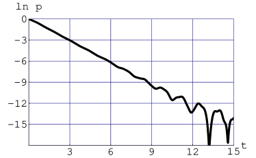
Figure 2: Survival probability as a function of time for $\Delta_{0}=.02$.

For $\Delta=.1$ (see Fig. 3) the FGR regime is seen up to $t=3$.

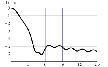
Figure 3: Survival probability as a function of time for $\Delta_{0}=.1$.

For $\Delta_{0}=.2$ (see Fig. 4) the FGR regime is absent.

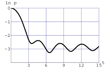
Figure 4: Survival probability as a function of time for $\Delta_{0}=.2$.

The Rabi oscillations we see already at Fig. 3 and still more vividly at Fig. 4.

As a second (and more physical) example consider a site coupled to a semi-infinite lattice longhi ; visuri . The system is described by the tight-binding Hamiltonian

$$H=-\frac{1}{2}\sum_{n=1}^{\infty}\big{(}\left|n\right>\left<n+1\right|+\left|n+1\right>\left<n\right|\big{)}$$

$$+\epsilon\left|d\right>\left<d\right|-V\big{(}\left|d\right>\left<1\right|+\left|1\right>\left<d\right|\big{)},$$ (34)

where $\left|n\right>$ is the state localized at the $n$-th site of the lattice. The band (lattice) states are described by the Hamiltonian

$$H_{0}=-\sum_{k}\cos k\left|k\right>\left<k\right|,$$ (35)

where $\left|k\right>=\sqrt{2N}\sum_{n}\sin(kn)\;\left|n\right>$. Hence we regain Hamiltonian (1) with $V_{k}=-\sqrt{2}V\sin k$. After simple algebra we obtain (in the upper half plain)

$$\Sigma(\omega)=\Delta_{0}\left(\omega-\sqrt{\omega^{2}-1}\right),$$ (36)

where the square root is defined as having the phase $\pi/2$ just above the real axis between $-1$ and $1$, and $\Delta_{0}=2V^{2}$. We immediately see that the GF for this model is a double valued function, the branch points being $+1$ and $-1$. The poles are given by the equation

$$\omega_{1,2}=\frac{\epsilon(1-\Delta_{0})\pm\Delta_{0}\sqrt{\epsilon^{2}-1+2\Delta_{0}}}{1-2\Delta_{0}}.$$ (37)

One sheet has real poles for $\Delta_{0}\geq(\epsilon^{2}+1)/2$. For $\Delta_{0}=(\epsilon^{2}-1)/2$ the GF has a second order pole at $\omega=(\epsilon^{2}+1)/2\epsilon$. When $\Delta_{0}$ increases, this second order pole is split into two first order poles, one going right (we assume $\epsilon>0$) and at $\Delta_{0}=1/2$ becoming a pole at the infinity. For $\Delta_{0}>1/2$ this pole appears for $\omega<-1$. The second first order pole, when $\Delta_{0}$ increases initially approaches the point $\omega=1$, and at a further increase of $\Delta_{0}$ moves in the opposite direction and asymptotically goes to infinity.

For $\Delta_{0}<(\epsilon^{2}+1)/2$ the second sheet has two complex poles of the first order. For $\Delta_{0}\ll 1$ the pole in the lower half-plain is situated at $\epsilon-i\Delta_{0}\sqrt{1-\epsilon^{2}}$ and is just the FGR pole mentioned above. The poles position is presented on Fig. 5.

Figure 5: Position of poles of the GF for the Hamiltonian (II) for different values of $\Delta$. The real poles appear on the standard sheet, the complex poles on the second sheet.

If we consider the case $\epsilon=0$ and $V^{2}/2<1$ the locator does not have real poles, so Eq. (12) after substitution of the results of Eq. (36) gives the amplitude of the non-decay amplitude longhi :

$$g(t)=\frac{1}{2\pi}\int_{-\pi}^{\pi}dQ\exp(it\cos Q)\frac{1-\exp(-2iQ)}{1+\alpha^{2}\exp(-2iQ)},$$ (38)

where $\alpha^{2}=1-\Delta_{0}$.

III Analytic continuation

For tunneling into continuum the points $E_{b}$ and $E_{t}$ are the $\Sigma(\omega)$ (and hence the propagator (7)) branch points. Hence propagator is a multi-valued function and it’s value in the lower half-plane depends upon the curve along which we continue the function from the upper half-plane silverman . The standard analytic continuation we used previously, consists of making the cut along the straight line between the branch points and considering only one sheet, thus making the analytic continuation into the lower $\omega$ half-plain by continuing $\Sigma(\omega)$ along the curves which circumvent the right branch point clockwise and the and the left branch point anti-clockwise.

On the other hand, we could use a different continuation, making the cuts from the branch points to infinity and continuing the function between the cuts along the curves passing through the part of real axis between $E_{b}$ and $E_{t}$, and outside as we did it previously. This way to make analytic continuation, and hence to calculate the integral (6) is presented on Fig. 6. (Of course, the value of the integral does not depend upon the analytic continuation we use.)

Figure 6: Alternative way to analytically continue the propagator into the lower half-plane. The arrows show the curves of analytical continuation in between the cuts and outside. Radius of the big arc and length of the cuts go to infinity.

(The treatment of tunneling from the discrete level into a semi-bound continuum presented in the paper by Onley and Kumar onley , corresponds, in fact, to an analytic continuation similar in spirit, to that presented on Fig. 6.) Notice, that because of the exponential decrease as a function of $t$ of the integrand in the cut integrals appearing in this analytic continuation, in contrast to oscillatory behavior of the real axis cut integral, such analytic continuation is more convenient for the numerical calculations of the large $t$ behavior of the non-decay amplitude.

For the alternative analytic continuation, Eq. (27) which is valid in the perturbative regime near the point $\omega=\epsilon$ in the upper half-plane is valid in lower half-plain also, thus giving a pole in a different sheet of the multivalued propagator. A simple illustration of the fact that the complex pole is present on the sheet of the propagator presented on Fig. 6, but not on that presented on Fig. 1 is obtained in the perturbative regime. In the lower half-plane in the vicinity of $\omega=\epsilon$ the standard propagator is

$$g(\omega)=\frac{1}{\omega-\epsilon-\Sigma^{\prime}(\epsilon)-i\pi\Delta(\epsilon)},$$ (39)

and the propagator continued according to Fig. 1 is

$$g(\omega)=\frac{1}{\omega-\epsilon-\Sigma^{\prime}(\epsilon)+i\pi\Delta(\epsilon)}.$$ (40)

Thus only the second propagator has (in a perturbative regime) a FGR pole.

IV Conclusions

In this paper we solve the problem of tunneling from a discrete level into continuum. We show, how the basic notion of the GF formalism, like frequency dependent discrete level propagator, self energy and spectral density, appear within the basic quantum mechanics. We concentrate on the calculation of the time dependent non-decay amplitude, the stage which is typically not given proper attention to within the GF formalism mahan . We show that the exponential time dependence of the non-decay probability given by the FGR is an approximation valid in perturbative regime and only for intermediate times. The large time dependence of the non-decay probability depends crucially upon the details of the band structure and hybridization interaction. We also look closely at those analytic properties of the propagator in the complex $\omega$ plane, which often pass unnoticed.

V Acknowledgements

The paper was finalized during the author’s visit to Max-Planck-Institut fur Physik komplexer Systeme, Dresden. The author cordially thanks the Institute for the hospitality extended to him during that and all his previous visits.

The author wishes to thank M. Katsnelson for the discussions which, in fact, triggered this work, and R. Gol and H. Elbaz for their constant interest.

VI Appendix

To generalize Eq. (20) to the case of non-interacting Fermi gas at finite temperatures, let us present the Hamiltonian (1) using second quantization

$$H=\sum_{k}\omega_{k}c_{k}^{\dagger}c_{k}+\epsilon d^{\dagger}d+\sum_{k}\left(V_{k}c_{k}^{\dagger}d+h.c.\right),$$ (41)

where $c_{k}^{\dagger}(c_{k})$ and $d^{\dagger}(d)$ are creation (annihilation) operators of band states and discrete state respectively. The tunneling of either the electron or the hole from the discrete level into continuum is described by Green’s functions $G^{>}$ and $G^{<}$ respectively mahan

$$G^{>}(t) = \left<d(t)d^{\dagger}(0)\right>$$

$$G^{<}(t) = \left<d^{\dagger}(t)d(0)\right>.$$ (42)

where the averaging is with respect to the grand canonical ensemble, and $d(t)$ or $d^{\dagger}(t)$ is the annihilation or the creation operator in Heisenberg representation. Both Green’s functions are simply connected with the spectral density function mahan

$$G^{>}(\omega) = [1-n_{F}(\omega)]A(\omega)$$

$$G^{<} = n_{F}(\omega)A(\omega),$$ (43)

where $n_{F}(\omega)=\left(e^{\beta(\omega-\mu)}+1\right)^{-1}$ is the Fermi distribution function ($\mu$ is the chemical potential and $\beta$ is the inverse temperature). Thus we obtain

$$G^{>}(t) = \int_{E_{b}}^{E_{t}}\frac{\Delta(E)[1-n_{F}(E)]e^{-iEt}dE}{\left[E-\epsilon-\Sigma^{\prime}(E)\right]^{2}+\pi^{2}{\Delta^{2}(E)}}$$

$$+ \sum_{j}[1-n_{F}(E_{j})]R_{j}$$

$$G^{<}(t) = \int_{E_{b}}^{E_{t}}\frac{\Delta(E)n_{F}(E)e^{-iEt}dE}{\left[E-\epsilon-\Sigma^{\prime}(E)\right]^{2}+\pi^{2}{\Delta^{2}(E)}}$$ (44)

$$+ \sum_{j}n_{F}(E_{j})R_{j}.$$

References

- (1) C. Cohen-Tannoudji, B. Diu, and F. Laloe, Quantum Mechanics, (Wiley, New York, 1977), vol.2, pp. 1344.
- (2) L. A. Khalfin, ”Contribution to the decay theory of a quasi-stationary state”, Sov. Phys. JETP 6, 1053-1063 (1958).
- (3) L. Fonda, G. C. Ghirardi, and A. Rimini, ”Decay theory of unstable quantum systems”, Rep. Prog. Phys. 41, 587-631 (1978).
- (4) H. Nakazato, M. Namiki, and S. Pascazio, ”Temporal behavior of quantum mechanical systems”, Int. J. Mod. Phys. B 10, 247-295 (1996).
- (5) G. D. Mahan, Many-Particle Physics, (Plenum Press, New York and London, 1990).
- (6) U. Fano, Phys. Rev. 124, 1866 (1961).
- (7) E. Kogan, arXiv:quant-ph/0609011; arXiv:quant-ph/0611043.
- (8) E. Kogan, HAIT Journal of Science and Engineering A, 5, 174 (2008).
- (9) A.-M. Visuri, C. Berthod, and T. Giamarchi, Phys. Rev. A 9, 053607 (2018).
- (10) V. N. Smelyanskiy, K. Kechedzhi, S. Boixo, S. V. Isakov, H. Neven, and B. Altshuler, arXiv:1802.09542 [quant-ph].
- (11) K. Kechedzhi, V. Smelyanskiy, J. R. McClean, V. S. Denchev, M. Mohseni, S. Isakov, S. Boixo, B. Altshuler, H. Neven, arXiv:1807.04792 [quant-ph].
- (12) S. Longhi, ”Nonexponential decay via tunneling in tight-binding lattices and the optical Zeno effect”, Phys. Rev. Lett. 97, 110402-1-110402-4 (2006).
- (13) R. A. Silverman, Complex Analysis with Applications, (Courier Dover Publications, 1984).
- (14) D. S. Onley and A. Kumar, ”Time dependence in quantum mechanics - Study of a simple decaying system”, Amer. J. Phys. 60, 432-439 (1992).